Networks and Cities: An Information Perspective

Abstract

Traffic is constrained by the information involved in locating the receiver and the physical distance between sender and receiver. We here focus on the former, and investigate traffic in the perspective of information handling. We re-plot the road map of cities in terms of the information needed to locate specific addresses and create information city networks with roads mapped to nodes and intersections to links between nodes. These networks have the broad degree distribution found in many other complex networks. The mapping to an information city network makes it possible to quantify the information associated with locating specific addresses.

Traffic and communication between different parts of a complex system are fundamental elements in maintaining its overall cooperation. Because a complex system consists of many different parts, it matters where signals are transmitted. Thus signaling and traffic is in principle specific, with each message going from a unique sender to a specific recipient. One example is living cells, where macromolecules are transported between cellular components and along micro-tubular highways to perform or direct actions on other particular macromolecules hartwell . This complicated cellular machinery is often simplified to a molecular network that maps out the signaling pathways in the system. We here will consider a city in a similar perspective, with communication defined by people that travel from one specific street to another. In many cases, the actual traveling distance could easily be less restrictive for communication than the amount of information needed to locate the correct address. In this work we will take this perspective to the extreme, and assume that the travel time/cost of just driving along a given road is zero. Accordingly we remap a city map to a dual information representation jiang : an information city network (Fig. 1). Subsequently we will use this network to estimate the information needed to navigate in a city, and thereby quantify and compare the complexity of cities.

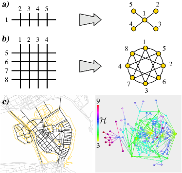
Figure 1: Mapping cities (left panels) into information networks (right panels). In (a) we show how a city consisting of one major street and 4 smaller streets maps to a single hub. This network represents the information handling you perform when you orient in such a city. On the major road 1 you need to know which of the exits 2-5 to take to get to the correct street: this corresponds to an information of $\log_{2}(4)=2$ bits. In (b) we show the city map of a very planned city, where each street intersects with many perpendicular streets. For example, it is very easy to go from an north-south (ns) street to another parallel ns street. A perpendicular east-west street is first reached with probability $1/4$. Next a ns is reached with probability $1/3$, if by assumption a just visited street is not visited again. There are four possible paths to the target street and therefore one only needs $-\log_{2}(4\frac{1}{4}\frac{1}{3})=\log_{2}(3)$ bits of information to go between two parallel streets (see Eq. (4)). In (c) we map “Gamla stan” in Stockholm, Sweden, to an information city network. Nodes are roughly positioned at the geographical position of the corresponding street and color coded according to the typical amount of information $\mathcal{H}$ needed to locate them.

Imagine that you want to get to a specific street in the city you are living in. If you have lived in the city for some time, you probably know how to find the street, and driving to the destination does not cost any new information. However, if you are new in the city, you need travel directions along the way to the target. In this paper we discuss the information value of such travel directions, or equivalently, we quantify the information associated to knowing the city you live in.

Assume that you get your travel directions in the form of the sequence of roads that will lead you to the target road. These roads form a path of roads with subsequent intersections. In network language, your trajectory can be mapped to a path in an “information city network”, where roads map to nodes and intersections between roads map to links between the nodes. This network represents an information view of the city, where distances along each road are effectively set to zero because it does not demand any information handling to drive between the crossroads.

In Fig. 1(a and b) we present two simple examples of two caricature cities mapped to such information networks. Fig. 1(a) shows a particular simple city consisting of a main road, that together with a collection of smaller roads define the city. This maps into a single hub, where all information handling consists in specifying which of the 4 side roads that is the right one. In Fig. 1(b) we show a slightly more elaborate city, that resembles modern planned cities. In that case any street can be accessed from a random perpendicular street, and effectively the information associated to locate a specific street is also small.

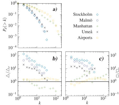
Figure 2: Characterizing traffic networks in terms of degree distribution (a), and number of short loops (b and c). $P_{d}(>k)$ is the probability that a node has degree $k$ or higher. Hence, it is the cumulative degree distribution that is plotted in (a). In (b) we show number of loops of length 3, $\triangle$, that nodes of degree $k$ participate in, normalized by what this number of loops would be in a randomized version of the network, $\triangle_{r}$, with 100 realizations. The random network is constructed such that the degree of every node is conserved, and such that the network remains globally connected maslov2002 . (c) shows the similarly normalized number of loops of length 4, $\Box$. Both types of loops tend to be over-represented in real city networks compared to the randomized ones. This reflects locality in the city networks.

In Fig. 1(c) we show a part of a real city, “Gamla stan” in Stockholm teleadress , Sweden, mapped to an information network. Long roads with many intersections are mapped to major hubs: The network representation nicely captures that the long roads are important for the overall traffic in the system. For a more systematic study we map a number of different cities to their information network counterpart, and examine their basic topological properties (Fig. 2). For comparison we also show another transportation network, consisting of airports in USA, connected by a link in case there is a direct flight between them airport . In this network, the travel directions are decided in the airports and we therefore analyze it with the airports as nodes and the flights between airports as links.

For all city networks, and also for the airport network we observe broad connectivity distributions (Fig. 2(a). However, the local properties differ qualitatively between the city networks and the airport network. We quantify the locality by the number of small loops of length 3 (triangles $\triangle$), related to clustering eckmann ; newman2003 ; barabasi , and length 4 (squares $\square$) in Fig. 2(b and c) normalized by their expectation number in random networks with conserved degree distribution maslov2002 ; maslov2002b . The airport network is close to its random counterpart, whereas the city networks differ substantially from their random expectations. The airports are connected with little regards to geographical distance, whereas in the cities, in particular the short roads have relatively many loops and thus exhibit substantial degree of locality. Manhattan, selected to represent a planned city, differs from the other cities in having few triangles and an overabundance of squares associated especially to the many streets of connectivity $\sim$$15$ and $\sim$$100$ that, respectively, cross the city in east-west and north-south direction.

To characterize the ease or difficulty of navigation in different networks, we use the “Search Information” $S$ pnas . Imagine a network, in this case an information city network, where we start on a node (a street) $s$ and want to locate node $t$ (another street) somewhere else in a connected network with $N$ nodes (streets). Further, we want to locate $t$ through the shortest path, or if there are several degenerate shortest paths, we want to locate $t$ through any of them. Without prior knowledge, the information needed for locating a given exit from a node of connectivity $k$, is $\log_{2}(k)$. For each path $p(s,t)$ from $s$ to $t$ the probability to follow it is

$$P[p(s,t)]\;=\;\frac{1}{k_{s}}\;\;\prod_{j\;\in\;p(s,t)}\frac{1}{k_{j}-1},$$ (1)

with $j$ counting all nodes on the path until the last node before the target $t$ is reached. The factor $k_{j}-1$ instead of $k_{j}$ takes into account the information gained by following the path, and therefore reducing the number of exit links by one. Thus, the total probability to locate node $t$ along any of the degenerate shortest paths is

$$P(s\rightarrow t)=\sum_{\{p(s,t)\}}P[p(s,t)],$$ (2)

where the sum runs over all degenerate paths that connect $s$ and $t$. The total information value of knowing any one of the degenerate paths between $s$ and $t$ is therefore

$$S(s\rightarrow t)=-\log_{2}\sum_{\{p(s,t)\}}P[p(s,t)].$$ (3)

We immediately see that the existence of many degenerate shortest paths makes it easier to find $t$. We stress that $S$ should not be confused with entropy measures associated to the degree distribution sole , or measures related to the dominating eigenvector of the adjacency matrix demetrius . Instead $S$ is related to specific traffic in the system.

Let us for illustration return to the “square city” in Fig. 1(b), with $N$ streets divided in $N/2$ north-south ($ns$) streets, and $N/2$ east-west ($ew$) streets. Going from any $ns$ street to a particular $ew$ street demands information about which of the $N/2$ exits we must take. This information is $S(ns\rightarrow ew)=\log_{2}(N/2)$. On the other hand, if we want to go from one $ns$ street to another $ns$ street, we can take anyone of the $N/2$ $ew$ streets. Each path is thus assigned a probability $(2/N)[1/(N/2-1)]$. But there are in fact $N/2$ degenerate paths, and the total information cost for locating parallel roads in this square city reduces to

$$S(ns\rightarrow ns)\;=\;-\log_{2}(\frac{N}{2}\frac{1}{N/2}\frac{1}{N/2-1})=\log_{2}(N/2-1),$$ (4)

reflecting the fact that it does not matter which of the $ew$ roads one will use to reach the target road.

To characterize the overall complexity in finding streets we calculate the average search information

$$S\;=\;\frac{1}{N^{2}}\;\sum_{s=1}^{N}\sum_{t=1}^{N}S(s,t),$$ (5)

for a number of cities in Fig. 3. To evaluate the $S$-values, we for each network also calculate the corresponding $S_{r}$ for its randomized version. This random network is constructed such that the degree of each node is the same as in original network, and also such that the overall network remains connected maslov2002 . Thus, comparing $S$ with $S_{r}$ properly takes into account both the size of the network, its total number of links as well as the degree distribution, but not the geometrical constraints. The 2-dimensional constraint of a real city is absent in the randomization. In all cases, including the airline network, we observe that $S>S_{r}$. Thus all networks are more difficult to navigate than their random counterpart (Fig. 3(a)).

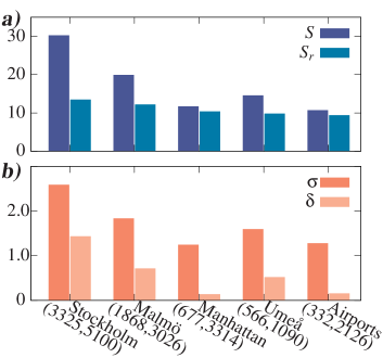
Figure 3: (a) shows the average information one needs to go from one specific street to another specific street for some city networks teleadress , and for the network of airports in USA connected by commercial airlines airport . ($N$,$L$) is, respectively, the number of nodes and links in the networks. In all cases we compare with the random counterpart of the network as described in the caption of Fig. 2. Overall we observe that Manhattan is more efficiently organized than the similar sized Umeå, but that both are relatively hard to navigate in compared with the US airport network. (b) shows the size-weighted search information $\sigma$ together with $\delta$, the corresponding difference with the randomized network.

To take size effects into account we from Eq. (4) expect that $S$ scales as $\log_{2}(N)$. We therefore define $\sigma=S/\log_{2}(N)$ to be able to compare cities of different sizes (Fig. 3(b)). Furthermore, $\delta=(S-S_{r})/\log_{2}(N)$ is interesting, since it measures how effectively the city is constructed given the length (degree) of the streets (Fig. 3(b)). According to Fig. 3(b) Manhattan is relatively easier to navigate in than the other cities. However, neither Manhattan is optimized. If Manhattan was constructed as a pure square city (Fig. 1(b)) the search information would be $S\sim 9$ according to Eq. (4).

To investigate what it is that makes it complicated to navigate in cities, we in Fig. 4 measure the information associated to nodes of different degrees in the network. We define the access information of a node $s$ by

$$\mathcal{A}_{s}=\frac{1}{N}\sum_{t}S(s,t),$$ (6)

where we sum over all target nodes $t$ in the network. The quantity $\mathcal{A}_{s}$ measures the average number of questions one needs to locate a specific street in the network, starting from node $s$. Thus $\mathcal{A}_{s}$ is a measure of how good the access to the network is from node $s$. In Fig. 4(a) we show $\langle\mathcal{A}(k)\rangle/\langle\mathcal{A}_{r}(k)\rangle$ averaged over all nodes of degree $k$ versus $k$. $\langle\mathcal{A}_{r}(k)\rangle$ is the average expectation of $\mathcal{A}(k)$ in a randomized network. Note that $\mathcal{H}_{t}=\frac{1}{N}\sum_{s}S(s,t)\neq\mathcal{A}_{t}=\frac{1}{N}\sum_{s}S(t,s)$. The difference reflects the asymmetry of the endpoints of a path. Imagine a small network that consists of a hub with five neighbors. The hub is easily reached from any of the neighbors. However, starting at the hub it is harder to reach a specific neighbor. The hub has low $\mathcal{H}$ and high $\mathcal{A}$ and the neighbors have high $\mathcal{H}$ and low $\mathcal{A}$.

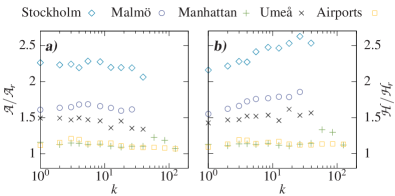
Figure 4: (a) shows the real-random access ratio $\langle\mathcal{A}(k)\rangle/\langle\mathcal{A}_{r}(k)\rangle$ and (b) shows the real-random hide ratio $\langle\mathcal{H}(k)\rangle/\langle\mathcal{H}_{r}(k)\rangle$. Overall they show similar qualitative behavior. Overall (a) and (b) show that the degree of a node plays a minor role for access $\mathcal{A}$ and hide $\mathcal{H}$.

The overall feature of Fig. 4(a and b) is that the positioning of the roads with respect to their degree does not explain the relatively high values of ${\cal H}$ and ${\cal A}$. However, the degree plays another indirect role: The presence of long roads shortens the distances in the information network and thereby decreases $S$, especially if degenerate paths exist. This is true for Manhattan and the network of airports, but not for the three Swedish cities according to their degree distributions (Fig. 2(a)). In the context of city planning, this suggests that for easy navigation it is often favorable to replace a big number of shorter streets with a few long, provided that they connect remote parts of the network.

When considering $\Delta S(l)=\langle S(l)\rangle_{pairs}-\langle S_{r}(l)\rangle_{pairs}$ as function of distances $l$ between nodes in the city networkfoot (not shown), we find that $\Delta S(l)<0$ for distances $l\sim 2$. This suggests that local navigation to a neighbor parallel road is optimized, whereas the $\Delta S(l)>0$ for $l>3$ reflects a tendency to protect local neighborhoods by hiding them. Thus the relatively large $S$ reflects a separation of these neighborhoods.

We also investigated the variance of $\mathcal{A}(k)$ and $\mathcal{H}(k)$ and found that this typically is much larger in real networks, compared to their random counterparts. This reflects the inhomogeneity in the organization of cities (Fig. 2(b and c)) with a fraction of streets being well hidden in remote corners of the cities. Such corners and local “islands”, overrepresented in Stockholm as a consequence of real islands, are essentially never present in the random counterparts. Many cities are organized hierarchical, where a few main streets connect to smaller streets, which in turn connects to even smaller streets. If a real city was organized purely hierarchical, with each street connected to one larger and two smaller streets, then $S=2\>log_{2}(N)$ for $N\rightarrow\infty$. In practice this hierarchical organization is partially broken by intersecting roads (decreasing $S$, e.g. Manhattan) and local neighborhoods or “islands” (increasing $S$, e.g. Stockholm). As a consequence $S\approx 2\>log_{2}(N)$ is only a rough estimate. Finally we have measured that locality in the form of an excess number of small loops (Fig. 2(b and c)) also contributes to $S-S_{r}$, since small loops introduce redundant paths without shortening distances substantially.

We have discussed the organization of cities in the perspective of communication and presented a way to remap a city map to a dual information representation. The information representation of a city opens for a way to quantify the value of knowing it: A large $S$ means that you have to know a lot to find your way around in a city as a newcomer. In another perspective it is an estimate of the asymmetry between traveling a way the first and second time, when travel time is included.

We have quantified the intuitive expectation that Manhattan, and presumably most modern planned cities are simple. In contrast, historical cities with a complicated past of cut and paste construction are more complex. The observation of a universally large $S$ relatively to $S_{r}$ in all networks we have investigated means that the ability to obtain information is relatively more important in these real world networks. Also it implies that city networks are not optimized for communication, as such an optimization would provide a topology with $S$ even smaller than $S_{r}$ (Fig. 1b). Rather the topologies of real cities, with high $S$, reflect a local tendency to avoid being exposed to non-specific traffic.

References

- (1) L. Hartwell, J. Hopfield, S. Leibler, and A. Murray, Nature (London) 402, C47 (1999).
- (2) B. Jiang, Environ. Plann. B. 31, 151 (2004).
- (3) S. Maslov and K. Sneppen, Science 296, 910 (2002).
- (4) TA Teleadress Information AB has kindly provided us with data for Stockholm and Malmö.
-
(5)
From Pajek datasets at:
http://vlado.fmf.uni-lj.si/pub/networks/data/ - (6) R. Albert and A.-L. Barabasi, Rev. Mod. Pys. 74, 47 (2002).
- (7) M. E. J. Newman, SIAM Review 45, 167 (2003).
- (8) J-P. Eckmann and E. Moses, Proc. Natl. Acad. Sci. U.S.A. 99, 5825 (2002).
- (9) S. Maslov, K. Sneppen and A. Zaliznyak, Physica A 333, 529 (2004).
- (10) K. Sneppen, A. Trusina and M. Rosvall, cond-mat/0407055
- (11) R. V. Sole and S. Valverde, in Complex Networks, edited by E. Ben-Naim, H. Frauenfelder and Z. Toroczkai, Lecture Notes in Phyics, 169. (Springer, Berlin, 2004).
- (12) L. Demetrius, Proc. Natl. Acad. Sci. U.S.A. 97, 3491 (2001).
- (13) The average runs over all pairs of nodes at distance .