Hide and seek on complex networks

Abstract

Signaling pathways and networks determine the ability to communicate in systems ranging from living cells to human society. We investigate how the network structure constrains communication in social-, man-made and biological networks. We find that human networks of governance and collaboration are predictable on teat-a-teat level, reflecting well defined pathways, but globally inefficient. In contrast, the Internet tends to have better overall communication abilities, more alternative pathways, and is therefore more robust. Between these extremes the molecular network of Saccharomyces cereviseae is more similar to the simpler social systems, whereas the pattern of interactions in the more complex Drosophilia melanogaster, resembles the robust Internet.

Information exchange between distant parts of a complex system is essential for its global functionality. For example, without the adaptability to environmental changes, maintained by communication through signaling pathways, perturbations would be fatal for living cells. Similarly, human society needs to maintain global cooperativity in order to be functional. No parts of such complex systems are complete, but all parts are in contact with each other through a network of distributed communication. The speed and reliability of the information transfer is closely linked to the network architecture (watts_strogatz, ; kleinberg, ; adamic, ; eckmann, ; dodds, ; rosvall, ). This interdependence can be characterized in terms of information measures and Shannon entropies (shannon, ). That is, we measure the number of bits of information required to transmit a message to a specific remote part of the network (Fig. 1a), or reversely, to predict from where a message is received (Fig. 1, b and c). We will thus represent information measures related to the network capacity for specific communication. The introduced measures are not to be confused by the Shannon entropies that have earlier been assigned to the network degree distribution (sole, ), respectively to the long time amplification of the dominant eigenvector of the network adjacency matrix (demetrius, ).

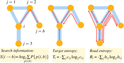
Figure 1: Information measures on network topology: (a) Search information $S(i\to b)$ measures your ability to locate node $b$ from node $i$. (b) Target entropy $T_{i}$ measures predictability of traffic to you located at node $i$, and (c) Road entropy $R_{i}$ measures predictability of traffic around $i$. $S(i\to b)$ is the number of yes/no questions needed to locate any of the shortest paths between node $i$ and node $b$. For each such path $P\{p(i,b)\}\;=\;\frac{1}{k_{i}}\;\;\prod_{j}\frac{1}{k_{j}-1}$, with $j$ counting nodes on the path $p(i,b)$ until the last node before $b$. $c_{ij}$ is the fraction of the messages targeted to $i$ that passed through neighbor node $j$. $b_{ij}$ is the fraction of messages that go through node $i$ which also go through neighbor node $j$.

In practice, imagine that you at node $i$ want to send a message to node $b$ in a given network (Fig. 1a). This could for example correspond to sending an E-mail over the Internet. For simplicity we assume that the message follow the shortest path, or if there are several degenerate shortest paths, it is sent along one of them. For each shortest path we calculate the probability to follow this path, Fig. 1a, if one without information would chose any new direction with equal probability:

$$P\{p(i,b)\}\;=\;\frac{1}{k_{i}}\;\;\prod_{j\;\in\;p(i,b)}\frac{1}{k_{j}-1},$$ (1)

with $j$ counting all nodes on the path from a node $i$ to until the last node before the target node $b$ is reached. The factor $k_{j}-1$ instead of $k_{j}$ takes into account the information we gain by following the path, and therefore reduce the number of exit links by one. The total information needed to identify one of all the degenerate paths between $i$ and $b$ defines the “search information”

$$S(i\rightarrow b)=-log_{2}\left(\sum_{p(i,b)}P\{p(i,b)\}\right),$$ (2)

where the sum runs over all degenerate paths that connect $i$ with $b$. A large $S(i\rightarrow b)$ means that one needs many yes/no questions to locate $b$. The existence of many degenerate paths will be reflected in a small $S$ and consequently in easy goal finding.

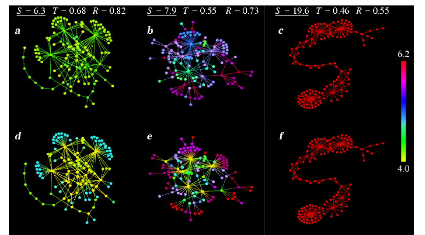
Figure 2: Hide and seek in complex networks. In (a-c) we show two networks obtained by (a) minimizing and (c) maximizing $S$, while keeping the degree distribution identical to the Canadian hardwired Internet in (b). This network was selected as a typical communication network (faloutsos, ; broder, ; barabasi, ), with a broad degree distribution $P(>k)\sim k^{-1.3}$. The color of each node $i$ shows the value ${\cal A}_{i}=\sum_{b}S(i\rightarrow b)$, that measures how easy it is to find other nodes when starting at node $i$. In (d-f) we show same networks, but color coded according to how difficult it is to find the nodes, $H_{b}=\sum_{i}S(i\rightarrow b)$.

The practical question is thus: Which position provides best access to the entire network? Surfing the Web, which web-page should be the start page when easy access to any other page is essential? The answer is the node with minimal access information, ${\cal A}_{i}=\sum_{b}S(i\rightarrow b)$. The networks in Fig. 2, a to c, are color coded according to ${\cal A}_{i}$. Fig. 2b illustrates that hubs, and often nodes directly connected to hubs, give best access to the system. Overall one can see that it is easy to access other nodes in the network in Fig. 2a, whereas it is much more difficult in Fig. 2c. In fact the network in Fig. 2b is the Canadian Internet (internet, ), whereas the networks in Fig. 2, a and c, are obtained by rewiring the Canadian network to, respectively, minimize and maximize $S=\sum_{i}{\cal A}_{i}/N$ while maintaining the network connected and conserving the degree of all nodes (maslov2002, ). $N$ is the number of nodes in the connected network.

Naturally, the next question is: Where it is best to hide? That is where ${\cal H}_{b}=\sum_{i}S(i\rightarrow b)$ is maximal. Note that maximizing everyone’s ability to hide $\sum_{b}{\cal H}_{b}=\sum_{i}{\cal A}_{i}=S\cdot N$ is equivalent to maximizing the search information and therefore minimizing everybody’s ability to search. Thus we illustrate the value of ${\cal H}_{b}$ in Fig. 2, d to f, for the same networks as in Fig. 2, a to c. In agreement with intuition we indeed find that hubs are easily accessible by other nodes and thus are bad places for hiding. Rather one should hide on nodes on the periphery. Is it possible for a node to have a good access to other nodes but not be easy accessible at the same time? The compromise favors a position on a neighbor to a hub. For example, if we consider the network implementation of a city with roads as nodes and intersections as links, it is preferable with an address on a small road that connects directly to a major road/hub.

We will later see that many real world networks are characterized by relatively high value of the overall search information $S$ (Fig. 4), implying that global search abilities are limited by functional, geographical or other constraints. The ability to search/hide is however not the only measure of the communication properties of a network. Another key aspect of communication handling is associated to prediction of local traffic to and across nodes in the network. This represents the “passive” aspect of information handling.

To define the predictability, let us consider messages arriving to a given node $i$ in a network. Your task, being on node $i$, is to guess the “active” neighbor/link from where the next message arrives. Without prior knowledge, all your local connections are equal and it would take you $\log_{2}(k)$ yes/no questions to guess the active link, where $k$ is the number of connections of your node. However, if the information about the traffic through links is available, the direction of the next message can be guessed with less questions if the search is biased towards the more used links. For simplicity we assume that all communication takes place through the shortest paths and all nodes communicate in equal amounts with all other nodes.

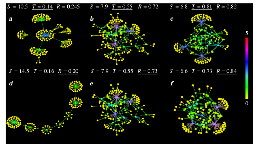
Figure 3: Prediction of local communication. The upper panel shows networks obtained by (a) minimizing and (c) maximizing the target entropy $T=\sum_{i}T_{i}/N$ associated to traffic to nodes in the networks, while keeping the degree distribution identical (maslov2002, ; maslov2002b, ) to the original network of Autonomous Systems in Canada shown in (b). (d to f) show the networks that (d) minimize and (f) maximize the road entropy $R=\sum_{i}R_{i}/N$ associated to traffic across nodes in the networks. In (a to c) the nodes are color coded according to the value of $T_{i}$, while we in (d to f) color code according to $R_{i}$.

The predictability, or alternatively the order/disorder of the traffic around a given node $i$, is measured by an entropy of messages that are targeted to a given node $i$, $T_{i}$, and an entropy of all messages across the node, $R_{i}$ (Fig. 1, b and c). The predictability based on the orders that are targeted to a given node $i$ is

$$T_{i}\;=\;-\sum_{j=1}^{k_{i}}c_{ij}log_{2}(c_{ij}),$$ (3)

where $j=1,2...,k_{i}$ denotes the links from node $i$ to its immediate neighbors $j$ and $c_{ij}$ is the fraction of the messages targeted to $i$ that passed through node $j$. Similarly we use $b_{ij}$, defined as the fraction of messages that go through node $i$ that also go through node $j$, to quantify the entropy associated to traffic across node $j$:

$$R_{i}\;=\;-\sum_{j=1}^{k_{i}}b_{ij}log_{2}(b_{ij}),$$ (4)

Technically $b_{ij}$ is proportional to the betweenness (between, ) of the link between $i$ and $j$, whereas $c_{ij}$ rather quantifies a sub-division of the network around node $i$. We will refer to $T_{i}$ as the target entropy, and to $R_{i}$ as the road entropy, where a large $T_{i}$ or $R_{i}$ mean a low predictability.

Fig. 3 shows the values of $T_{i}$ and $R_{i}$ for different complex networks. In Fig. 3, a to c, we examine networks by color coding the nodes according to target entropy, $T_{i}$. Fig. 3, d to f, show networks color coded according to the road entropy $R_{i}$. The bluish hubs reflect that traffic to highly connected nodes is hard to predict. However, this is not always the case: the location of nodes with low predictability also depends on the overall topology of the network. The networks in Fig. 3 are presented so that the entropy increases from, respectively, a and d to c and f. As the networks get more disorganized, the number of hubs with disordered traffic increases. Also, nodes of low degree become more confused as they tend to position themselves between the hubs. It is interesting that this positioning of low degree nodes increases the number of alternative pathways in the system, and thus tend to minimize the search information $S$. Therefore the minimal $S$ network in Fig. 2a is similar to the maximal $R=\sum_{i}R_{i}$ or $T=\sum_{i}T_{i}$ networks in Fig. 3, c and f.

Whereas the maximal $T$ and $R$ networks are topologically similar, this is not at all the case for the minimal $T$ and $R$ networks in Fig. 3, a and d. The network of minimal $T$ in Fig. 3a concentrates all signaling into a simple star like structure with hierarchical features (trusina2004, ). As a consequence nearly everybody can easily predict from where the next message will come. In contrast, minimizing $R$ results in a topology characterized by hubs on a string forming an “information super highway” (Fig. 3d). Thus a low road entropy $R$ means that relatively many links are important, whereas a large $R$ implies that few links are essential. In this sense $R$ is related to robustness in an intentional edge attack (newman2003, ) whereas $T$ reflects robustness in an intentional node attack (newman2003, ).

We apply our information measures to characterize real networks in Fig. 4, by comparing a number of networks with their randomized counterparts (maslov2002, ). The datails of the comparison is shown in table 1. For each network we show the Z-score for $S$, $T$ and $R$. A large positive $Z$-score means that the corresponding network has relatively large entropy. For example we see that the hardwired Internet is quite “messy” in all senses: The traffic is unpredictable, implying that the network is robust, and at the same time one needs relatively large information handling to transmit packages across the system. In contrast the social networks, exemplified here by the network of company executives in USA, CEO (ceo, ) and the scientific collaboration network, hep-th (th-hep, ), show a pronounced pattern of high traffic predictability and large cost of locating any particular node. These features are characteristic to the ordered network topologies in Fig. 3a and d.

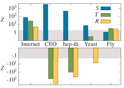
Figure 4: Measure of relative order in communication networks. A high $Z$-score implies relatively high entropy. In all cases we show $Z=(I-I_{r})/\sigma_{r}$ for the information measures $I=$ $S$, $T$ and $R$, by comparing with $I_{r}$ for randomized networks with preserved degree distribution. $\sigma_{r}$ is the standard deviation of the corresponding $I_{r}$, sampled over 100 realizations. Results within the shaded area of two standard deviations are insignificant. All networks have a relatively high search information $S$. The two human interaction networks CEO (ceo, ) and scientific collaborations (th-hep, ) show a distinct communication structure characterized by local predictability, low $T$ and $R$, and global inefficiency, high $S$.

In Fig. 4 we also investigate networks of physical interactions among proteins in two organisms, yeast (Uetz2000, ; Ito2001, ) and fly (giot, ). Whereas the fly network is quite close to its randomized counterpart, yeast is reminiscent of the social networks. The large $S$ for yeast reflects that many of the largest hubs are positioned on the periphery of the network (maslov2002, ), and therefore have relatively large entropy ${\cal A}_{i}$, see Fig. 5. This tendency of hub separation reflects optimization of local communication, at the cost of global specific signaling. On the other hand the protein network of the multicellular and more advanced fly, Drosophilia melanogaster, displays a more complicated and in fact more robust topology as witnessed by the significantly positive $Z-$scores for $T$ and $R$ entropies.

Table 1: Measure of order in communication networks. Five networks together with their size $N$ and the three information-entropy measures $I=S$, $T$ and $R$. In each case we compare the measured $I$-value by comparing with $I_{r}$ for randomized networks with preserved degree distribution. $\sigma_{r}$ is the standard deviation of the corresponding $I_{r}$ sampled over 100 realizations. For all networks we only consider the largest connected component, that is also maintained during the randomization. The Internet network is the hardwired Internet of autonomous systems (internet, ). The CEO network is chief executive officers connected by links when they sit in the same board of directors (ceo, ), hep-th is a network of scientists connected by links if they coauthor a publication (th-hep, ), yeast is the protein-protein interaction network in Saccharomyces Cerevisiae detected by the two-hybrid experiment(Uetz2000, ), and fly refers to the similar network in Drosophilia melanogaster (giot, ). Both of these networks are pruned to include only interactions of high confidence, and in both networks we compare with their random counterparts where both bait and prey connectivity of all proteins are preserved. The results on the network of (Uetz2000, ) is reproduced when considering the core of the yeast network measured by (Ito2001, ). Furthermore, all results are robust to a 10% random removal of links except for the fly network which with such a pruning tends to be closer to the yeast network.

Network	$N$	$S$		$T$		$R$
Internet	$6474$	$16$.	$34$	$0$.	$583$	$0$.	$809$
randomized		$15$.	$03(2)$	$0$.	$499(3)$	$0$.	$793(3)$
CEO	$6193$	$20$.	$693$	$1$.	$58$	$1$.	$831$
randomized		$12$.	$597(3)$	$3$.	$316(3)$	$3$.	$513(1)$
hep-th	$5835$	$19$.	$72$	$0$.	$847$	$1$.	$211$
randomized		$13$.	$48(1)$	$1$.	$385(5)$	$1$.	$668(1)$
Yeast (Uetz2000, )	$921$	$13$.	$3$	$0$.	$38$	$0$.	$722$
randomized		$12$.	$5(1)$	$0$.	$38(1)$	$0$.	$742(3)$
Yeast (Ito2001, )	$417$	$12$.	$2$	$0$.	$30$	$0$.	$662$
randomized		$10$.	$7(2)$	$0$.	$33(2)$	$0$.	$708(6)$
Fly	$2915$	$14$.	$03$	$0$.	$56$	$0$.	$931$
randomized		$13$.	$96(6)$	$0$.	$53(1)$	$0$.	$925(2)$

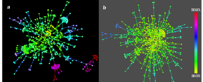
Figure 5: Analysis of the protein-protein interaction network in yeast: (a) shows the core of the yeast protein-protein interaction network color coded according to ${\cal A}_{i}$. The core data is the reliable subset of the two hybrid data set of Ito et al. (Ito2001, ), obtained by selecting the largest connected component of the network with only interactions with at least 3 IST included. The value of ${\cal A}_{i}$ is increasing from yellow through green and blue to red which mark nodes that have least access to the rest of the network. Proteins colored in red are proteins with “specific signaling pattern”. (b) shows an example of a randomized version of the network in (a), also color coded with the corresponding ${\cal A}_{i}$ values. The network is randomized such that the number of links for each node (protein) is maintained, while interaction partners are reshuffled in the same way as in the analysis leading to Fig. 4. The access information are substantially lower than in (a), reflecting a topology with better global access at the cost of higher possibility to be disturbed.

Networks are inherently coupled to communication and indeed their topology reflects this. The optimal topology for information transfer relies on a system-specific balance between effective communication (search) and not having the individual parts being unnecessarily disturbed (hide). We have presented measures that quantify the ease of global search, $S$, and the predictability of local activity, $T$ and $R$, and illustrated how they characterize the organization of complex networks.

In particular the network of corporate CEOs and scientific co-authorship, were found to be highly “predictable”, and at the same time very inefficient in transmitting information. In contrast the hardwired Internet was found to be locally unpredictable, and therefore robust against local failures. Finally the fruit fly, Drosophilia melanogaster, has a more robust protein network than yeast, Saccromyces cerevisiae, with better connections between distant parts of the network. This global communication optimization may reflect that the multicellular organism must sustain life in cells with many more different local environments than the single-celled yeast.

We thank R. Donangelo, P. Minnhagen and J. Wakeling for useful comments and revisions of the manuscript. We acknowledges the support of Swedish Research Council through Grants No. 621 2003 6290 and 629 2002 6258 and of EU through the Evergrow project.
Correspondence and requests for materials should be addressed to K. Sneppen (email: sneppen@nbi.dk).

References

- (1) Watts, D. & Strogatz, S. (1998) Nature 393, 400 .
- (2) Kleinberg, J. M. (2000) Nature 406, 845 .
- (3) Adamic, L. A., Lukose, R. M., Puniyani, A. R., Huberman, B. A. (2001) Phys. Rev. E 64 046135.
- (4) Eckmann, J-P. & Moses, E. (2002) Proc. Natl. Acad. Sci. U.S.A. 99, 5825.
- (5) Dodds, P. S., Muhamad, R., Watts, D. J. (2003) Science 301, 827.
- (6) Rosvall, M. & Sneppen, K. (2003) Phys. Rev. Lett. 91, 178701.
- (7) Shannon, C. E., Weaver, W. (1963) The Mathematical Theory of communication (Univ. of Illinois, Champaign, IL).
- (8) Sole, R. V., & Valverde, S. (2004) Information Theory of Complex Networks In: Complex Networks, E. Ben-Naim, H. Frauenfelder, and Z. Toroczkai (eds.), Lecture Notes in Phyics, pp 169-190. Springer, Berlin .
- (9) Demetrius, L. (2001) Proc. Natl. Acad. Sci. U.S.A. 97, 3491-3498.
- (10) Newman, M. E. J. (2001) Phys. Rev. E 64, 016132.
- (11) Faloutsos, M., Faloutsos, P., Faloutsos, C. (1999) Comput. Commun. Rev. 29, 251.
- (12) Broder, A., Kumar, B., Maghoul, F., Raghavan, P., Rajagopalan, S., Stata, R., Tomkins, A., Wiener, J. (2000) Computer Networks 33, 309.
- (13) Albert, R. & Barabasi, A.-L. (2002) Rev. Mod. Pys. 74, 47.
- (14) Maslov, S., & Sneppen, K. (2002) Science 296, 910.
- (15) Maslov, S., Sneppen, K., Zaliznyak, A. (2004) Physica A 333, 529.
- (16) Trusina, A., Maslov, S., Sneppen, K., Minnhagen, P. (2004) Phys. Rev. Lett. 92, 178702.
- (17) Newman, M. E. J. (2003) SIAM Review 45, 167.
- (18) Davis, G. F. & Greve, H. R. (1997) American Journal of Sociology 103, 1.
- (19) Newman, M. E. J. (2001) Phys. Rev. E 64, 016131.
- (20) Website maintained by the NLANR Measurement and Network Analysis Group at http://moat.nlanr.net/
- (21) Uetz, P. et al (2000) Nature 403, 623.
- (22) Ito, T., Chiba, T., Ozawa, R., Yoshida, M., Hattori, M., Sakaki, Y. (2001) Proc. Natl. Acad. Sci. U.S.A. 98, 4569.
- (23) Giot, L. et al. (2003) Science 302, 1727.