Ultimate Fate of Constrained Voters

Abstract

We determine the ultimate fate of individual opinions in a socially-interacting population of leftists, centrists, and rightists. In an elemental interaction between agents, a centrist and a leftist can become both centrists or both become leftists with equal rates (and similarly for a centrist and a rightist). However leftists and rightists do not interact. This interaction step between pairs of agents is applied repeatedly until the system can no longer evolve. In the mean-field limit, we determine the exact probability that the system reaches consensus (either leftist, rightist, or centrist) or a frozen mixture of leftists and rightists as a function of the initial composition of the population. We also determine the mean time until the final state is reached. Some implications of our results for the ultimate fate in a limit of the Axelrod model are discussed.

I Introduction

A basic issue in social dynamics is to understand how opinion diversity arises when interactions between individuals are primarily “ferromagnetic” in character. Many kinetic spin models have been proposed to address this general question G ; LN97 ; W ; Sz ; KR . An important example of this genre is the appealingly simple Axelrod model axelrod ; CMV , which accounts for the formation of distinct cultural domains within a population. In the Axelrod model, each individual is endowed with a set of features (such as political leaning, music preference, choice of newspaper, etc.), with a fixed number of choices for each feature. Evolution occurs by the following voter-model-like update step voter . A random individual is picked and this person selects an interaction partner (anybody in the mean-field limit, and a nearest-neighbor for finite spatial dimension). For this pair of agents a feature is randomly selected. If these agents have the same state for this feature, then another feature is picked and the initial person adopts the state of this new feature from the interaction partner. This dynamics mimics the feature that individuals who share similar sentiments on lifestyle issues can have a meaningful interaction in which one will convince the other of a preference on an issue where disagreement exists.

Depending on the number of traits and the number of states per trait, a population may evolve to global consensus or it may break up into distinct cultural domains, in which individuals in different domains do not have any common traits axelrod ; CMV . This diversity is perhaps the most striking feature of the Axelrod model. An even simpler example with a related phenomenology is the bounded compromise model Deff ; HK ; BKR . Here, each individual possesses a single real-valued opinion that evolves by compromise. In an update step, two interacting individuals average their opinions if their opinion difference is within a pre-set threshold. However, if this difference is greater than the threshold, there is no interaction. These steps are repeated until the system reaches a final state. For a sufficiently large threshold the final state is consensus, while for a smaller threshold the system breaks up into distinct opinion clusters; these are analogous to the cultural domains of the Axelrod model.

In spite of the simplicity of these models, most of our understanding stems from simulation results. As a first step toward analytic insight, a discrete three-state version of the bounded compromise model was recently introduced VKR . This is perhaps the simplest opinion dynamics model that includes the competing features of consensus and incompatibility. This model was found to exhibit a variety of anomalous features in low dimensions, including slow non-universal kinetics and power-law spatial organization of single-opinion domains. In this work, we focus on the ultimate fate of this system in the mean-field limit. We determine the exact probability that the final state of the system is either consensus or a frozen mixture of leftists and rightists as a function of the initial composition of the system. We also compute the time required for the system to reach its ultimate state.

In the next section, we define our model, outline its basic properties, and determine the ultimate fate of the system in terms of an equivalent first-passage process. The solution to this problem is used to obtain the probabilities of reaching either a frozen final state (Sec. III) or consensus (Sec. IV). In Sec. V, we compute the mean time until the final state is reached. In the discussion section, we generalize to non-symmetric interactions and also show how our results can be adapted to determine the ultimate fate of a version of the Axelrod model. Calculational details are presented in the appendices.

II The Model

We consider a population of $N$ individuals, or agents, that are located at the nodes of a graph. Each agent can be in one of three opinion states: leftist, centrist, or rightist. As shown in Fig. 1, we represent these states as $-,0$, and $+$, respectively. In a single microscopic event an agent is selected at random. We consider the mean-field limit in which the neighbor of an agent can be anyone else in the system. If the two agents have the same opinion, nothing happens. If one is a centrist and the other is an extremist (or vice versa), the initial agent adopts the opinion of its neighbor — that is, each individual can be viewed as having zero self-confidence and merely adopts the state of a compatible neighbor; this kinetic step is the same as in the classical voter model voter . However, if the two agents are extremists of opposite persuasions, they are incompatible and do not influence each other. As a result of this incompatibility constraint, the final state of the system can be either consensus of any of the three species, or a frozen mixture of leftist and rightist extremists, with no centrists.

Figure 1: Update events for different pair states.

In a mean-field system with $N_{-}$ leftists , $N_{+}$ rightists, and $N_{0}$ centrists (with $N_{+}+N_{-}+N_{0}=N$), the probability of selecting a pair $ij$ ($i,j=+,-,0$) equals $2N_{i}N_{j}/[N(N-1)]$, where $N_{i}$ is the number of agents of type $i$. Then the elemental update steps and their respective probabilities are:

$$(N_{-},N_{0})\to(N_{-}\!\pm\!1,N_{0}\!\mp\!1) {\rm prob.} p_{x}=\frac{N_{-}N_{0}}{N(N-1)}$$

$$(N_{+},N_{0})\to(N_{+}\!\pm\!1,N_{0}\!\mp\!1) {\rm prob.} p_{y}=\frac{N_{+}N_{0}}{N(N-1)},$$

while the probability for no change is $1-2(p_{x}+p_{y})$.

Figure 2: The density triangle $x+y+z=1$. The heavy dots denote consensus states and the heavy line denotes the frozen final states where no centrists remain. Typical random walk trajectories are shown, along with their projections (dashed) on the $z=0$ plane. When a random walk reaches the lines $x=0$ or $y=0$, the random walk subsequently must remain on this line until consensus is reached. The corresponding hopping probabilities on the $z=0$ plane are also indicated.

Eventually the system reaches a static final state that is either consensus of one of the three species or a frozen mixture of leftists and rightists. Monte Carlo simulations showed that the nature of the final state has a non-trivial dependence on the initial densities of the species VKR . We now analytically determine this final state probability as a function of the initial population composition by solving an equivalent first-passage problem. As shown in Fig. 2, the state of the system corresponds to a point in the space of densities $x=N_{-}/N$, $y=N_{+}/N$, and $z=N_{0}/N$. Since $x+y+z=1$, this constraint restricts the system to the triangle $ABD$ shown in the figure.

When two agents interact, the state of the system may change and we can view this change as a step of a corresponding random walk on the triangle $ABD$, with single step hopping probabilities given in Eq. (II). When the walk reaches one of the fixed points $A$, $B$, or $D$ (consensus), or any point on the fixed line $AB$ (frozen extremist mixture), the system stops evolving. This set represents absorbing boundaries for the effective random walk. Thus to find the probability of reaching a given final state, we compute the first-passage probability for the random walk to hit a given absorbing boundary.

We may simplify the problem by using the fact that only two of the densities $(x,y,z)$ are independent. We thus choose $x$ and $y$ as the independent variables by projecting the effective random walk trajectory onto the $z=0$ plane (Fig. 2). According to Eq. (II), this two-dimensional random walk jumps to its nearest neighbors in the $x$ and $y$ directions with respective probabilities $p_{x}=xz/(1-\delta)\approx xz$ and $p_{y}=yz/(1-\delta)\approx yz$, and stays in the same site with probability $1-2(p_{x}+p_{y})$. Here $\delta=1/N$, and we consider the limit $N\to\infty$.

III Frozen Final State

We now determine the probability $P_{+-}(x,y)$ for the system to reach a frozen state when the initial densities are $\rho_{-}(t=0)\equiv x$ and $\rho_{+}(t=0)\equiv y$. This coincides with the first-passage probability for the equivalent random walk to hit the line $x+y=1$ when it starts at a general point $(x,y)$ in the interior of the triangle. There are also absorbing boundaries on the sides $x=0$ and $y=0$, where the probability of reaching the frozen state is zero, and $P_{+-}(x,y)=1$ on the line segment $x+y=1$. For notational simplicity, we write $F(x,y)\equiv P_{+-}(x,y)$. In the equivalent random walk process, this first-passage probability obeys the recursion redner

$$F(x,y) = p_{x}[F(x-\delta,y)+F(x+\delta,y)]$$ (2)

$$+ p_{y}[F(x,y-\delta)+F(x,y+\delta)]$$

$$+ [1-2(p_{x}+p_{y})]F(x,y).$$

That is, the first-passage probability $F(x,y)$ equals the probability of taking a step in some direction (the factor $p_{i}$) times the first-passage probability from this target site to the boundary. This product is then summed over all possible target sites after one step of the walk.

In the continuum limit ($N\rightarrow\infty$) we expand this equation to second order in $\delta$ and obtain

$$x\frac{\partial^{2}F(x,y)}{\partial x^{2}}+y\frac{\partial^{2}F(x,y)}{\partial y^{2}}=0,$$ (3)

supplemented with the boundary conditions

$$F(x,0)=0$$

$$F(0,y)=0$$

$$F(x,1-x)=1.$$

The solution to Eq. (3) is not straightforward because of the mixed boundary conditions. Instead of attacking the problem directly, we transform to the coordinates $u=\sqrt{x}$, $v=\sqrt{y}$ to map the triangle to a quarter-circle of unit radius and then apply separation of variables in this geometry.

The transformed differential equation is

$$\frac{\partial^{2}F(u,v)}{\partial u^{2}} + \frac{\partial^{2}F(u,v)}{\partial v^{2}}$$ (4)

$$- \frac{1}{u}\frac{\partial F(u,v)}{\partial{u}}-\frac{1}{v}\frac{\partial F(u,v)}{\partial{v}}=0.$$

Because of the circular symmetry of the boundary conditions in this reference frame, it is now convenient to use the polar coordinates $(\rho,\theta)$, where $u=\rho\cos\theta$ and $v=\rho\sin\theta$. This transforms Eq. (4) to

$$\frac{\partial^{2}F(\rho,\theta)}{\partial\rho^{2}} - \frac{1}{\rho}\frac{\partial F(\rho,\theta)}{\partial{\rho}}+\frac{1}{\rho^{2}}\frac{\partial^{2}F(\rho,\theta)}{\partial{\theta^{2}}}$$ (5)

$$+ \frac{1}{\rho^{2}}\left(\tan\theta-\cot\theta\right)\frac{\partial F(\rho,\theta)}{\partial\theta}=0$$

We seek a product solution $F(\rho,\theta)=R(\rho)\Theta(\theta)$. Substituting this into Eq. (5) leads to the separated equations

$$\frac{d^{2}R}{d\rho^{2}}-\frac{1}{\rho}\frac{dR}{d\rho}-\frac{m^{2}}{\rho^{2}}R=0$$ (7)

$$\frac{d^{2}\Theta}{d\theta^{2}}+\left(\tan\theta-\cot\theta\right)\frac{d\Theta}{d\theta}+m^{2}\Theta=0$$

where $m$ is the separation constant.

Eq. (7) is equidimensional and thus has the general power-law form

$$R(\rho)=A_{+}\rho^{1+\sqrt{1+m^{2}}}+A_{-}\rho^{1-\sqrt{1+m^{2}}}$$ (8)

where $A_{\pm}$ are constants. To solve Eq. (7), we proceed by eliminating the first derivative to give a Schrödinger-like equation. Thus we define $\Theta(\theta)\equiv f(\theta)\,u(\theta)$ and find the function $f(\theta)$ that eliminates this first derivative term.

Substituting $\Theta=f\,u$ in Eq. (7) gives

$$fu^{\prime\prime} + \left[2f^{\prime}+\left(\tan\theta-\cot\theta\right)f\right]u^{\prime}$$ (9)

$$+ \left[f^{\prime\prime}+\left(\tan\theta-\cot\theta\right)f^{\prime}+m^{2}f\right]u=0,$$

and the coefficient of $u^{\prime}$ is zero if $f$ satisfies

$$2f^{\prime}+\left(\tan\theta-\cot\theta\right)f=0,$$

whose solution is

$$f(\theta)\propto\sqrt{2\sin\theta\cos\theta}\propto\sqrt{\sin 2\theta}.$$ (10)

Substituting this expression for $f$ in Eq. (9), we obtain

$$\frac{d^{2}u}{d\theta^{2}}+\left[(1+m^{2})-\frac{3}{4}\left(\frac{1}{\sin^{2}\theta}+\frac{1}{\cos^{2}\theta}\right)\right]u=0.$$ (11)

Details of the solution to this Schrödinger equation are given in Appendix A. The final result is

$$F(\rho,\theta) = R(\rho)f(\theta)u(\theta)$$

$$= \sum_{n~{}{\rm odd}}\frac{(2n+1)}{n(n+1)}\;\rho^{2(n+1)}\,\sin 2\theta\,\,P_{n}^{1}\left(\cos 2\theta\right),$$

where $P_{n}^{1}$ is the associated Legendre function. We transform back to the original $xy$ coordinates through

$$u=\rho\cos\theta=\sqrt{x}\qquad v=\rho\sin\theta=\sqrt{y}$$

$$\sin 2\theta=\frac{2\sqrt{xy}}{x+y}\qquad\cos 2\theta=\frac{x-y}{x+y}$$

Finally, identifying $F$ with $P_{+-}$, the solution in the original Cartesian coordinates is

$$P_{+-}(x,y)=\sum_{n~{}{\rm odd}}\frac{2(2n+1)}{n(n+1)}\,\sqrt{xy}\,(x+y)^{n}\,P_{n}^{1}\left(\frac{x-y}{x+y}\right).$$ (13)

This gives the probability of reaching a final frozen state when the population has initial densities $x$ and $y$ of leftists and rightists, respectively. Notice that this probability is symmetric, $P_{+-}(x,y)=P_{+-}(y,x)$, because $P_{n}^{1}$ is an even function for $n$ odd and an odd function for $n$ even. This reflects the obvious physical symmetry that the probability $P_{+-}$ is invariant under the interchange of leftists and rightists.

For equal initial densities of leftists and rightists, namely $x=y=(1-z)/2$, Eq. (13) becomes a function of the initial density of centrists $z$ only

$$P_{+-}(z)=\sum_{n~{}{\rm odd}}\frac{(2n+1)}{n(n+1)}(1-z)^{n+1}\;P_{n}^{1}(0).$$

As shown in Appendix B, this can be simplified to the closed-form expression

$$P_{+-}(z)=1-\frac{1-(1-z)^{2}}{\sqrt{1+(1-z)^{2}}}$$ (14)

with $0\leq z\leq 1$. This solution is shown in Fig. 3 along with Monte-Carlo simulation results.

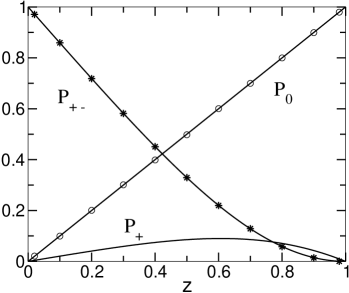
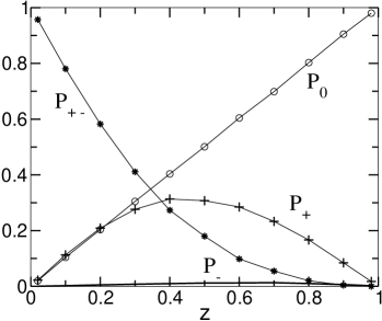
Figure 3: Probability of reaching the frozen final state, $P_{+-}$, and extremist consensus, $P_{+}$, as a function of the initial density of centrists $z$ for the case of equal initial densities of leftists and rightists, $y/x=1$ (top) and for the case $y/x=9$ (bottom).

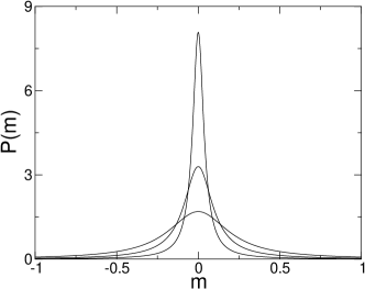
Figure 4: Probability distribution that an initially symmetric system $(x=y)$ has magnetization $m$ in the frozen final state, for the cases $z=0.04$, 0.1, and 0.2 (progressively broadening curves).

IV Consensus Final States

In addition to reaching a frozen final state, the system can also reach global consensus — either leftist, rightist, or centrist. Again, the probabilities for these latter three events depends on the initial composition of the system. We thus define $P_{-}(x,y)$, $P_{+}(x,y)$, and $P_{0}(x,y)$, as the respective probabilities to reach a leftist, rightist, or centrist consensus as a function of the initial densities.

The probability for centrist consensus can be obtained by elementary means. We merely map the 3-state constrained system onto the 2-state voter model by considering the leftist and rightist opinions as comprising a single extremist state, while the centrist opinion state maintains its identity. The dynamics of this system is exactly that of the classical 2-state voter model. Since the overall magnetization of the voter model is conserved voter , the probability that the system reaches centrist consensus, for a given $x$ and $y$ is simply

$$P_{0}(x,y)=z=1-(x+y).$$ (15)

To find the probability for leftist and rightist consensus, we use normalization of the final state probability

$$P_{+}(x,y)+P_{-}(x,y)+P_{+-}(x,y)+P_{0}(x,y)=1$$ (16)

and conservation of the global magnetization to write

$$y-x = P_{+}(x,y)-P_{-}(x,y)$$ (17)

$$+ \int_{0}^{1}(1-2x^{\prime})F(x^{\prime}|x,y)dx^{\prime}.$$

Here $F(x^{\prime}|x,y)$ is the probability of ending in a specific frozen state with density $x^{\prime}$ of $-$ spins and $1-x^{\prime}$ of $+$ spins as a function of the initial densities $x$ and $y$. This function therefore satisfies the normalization condition $P_{+-}(x,y)=\int_{0}^{1}F(x^{\prime}|x,y)dx^{\prime}$. Additionally the integral in Eq. (17) is the final magnetization in the frozen state. From the exact solution for $F(x^{\prime}|x,y)$ given in Eq. (38), we thereby obtain as a byproduct the magnetization distribution in the final frozen state (Fig. 4). As expected, for a small initial density of centrists $z$, there is little evolution before the final state is reached and the magnetization distribution is narrow.

Using Eq. (15) and the normalization condition for $F(x^{\prime}|x,y)$, we recast Eqs. (16) and (17) as

$$P_{+}(x,y)+P_{-}(x,y)+P_{+-}(x,y)=x+y,$$ (18)

and

$$P_{+}(x,y) - P_{-}(x,y)+P_{+-}(x,y)$$ (19)

$$- 2\int_{0}^{1}x^{\prime}F(x^{\prime}|x,y)dx^{\prime}=y-x.$$

Subtracting these equations, we obtain

$$P_{-}(x,y)=x-\int_{0}^{1}x^{\prime}F(x^{\prime}|x,y)dx^{\prime}$$ (20)

Now the first-passage probability $F(x^{\prime}|x,y)$ to a frozen state with a specified density $x^{\prime}$ of $-$ spins obeys the same differential equation as $P_{+-}$ [Eq. (3)], but with the boundary conditions

$$F(x^{\prime}|x,0) = 0$$

$$F(x^{\prime}|0,y) = 0$$

$$F(x^{\prime}|x,1-x) = \delta(x-x^{\prime})$$ (21)

The last condition states that the first-passage probability to the point $(x^{\prime},1-x^{\prime})$ on the boundary $x+y=1$ is zero unless the effective random walk starts at $(x^{\prime},1-x^{\prime})$. The first-passage probability $F(x^{\prime}|x,y)$ has the general form given in Eq. (34), but with the coefficients $c_{n}$ now determined from the boundary conditions in Eq. (21).

From the solution for $F(x^{\prime}|x,y)$ given in Appendix A, the probability of $-$ consensus as a function of the initial densities $x$ and $y$ is

$$P_{-}(x,y)=x-\sum_{n=1}^{\infty}\frac{(2n+1)}{n(n+1)}\,\sqrt{xy}\,(x+y)^{n}\,P_{n}^{1}\left(\frac{x-y}{x+y}\right)$$ (22)

The probability of $+$ consensus can be obtained by using the fact that $P_{+}(x,y)=P_{-}(y,x)$.

For the special case of $x=y=(1-z)/2$, the probabilities $P_{+}(z)=P_{-}(z)$ can be obtained either by setting $x=y$ in Eq. (22) and summing the series, or, more simply, by using Eq. (14) for $P_{+-}(z)$ and the probability conservation equation $2P_{+}(z)+P_{+-}(z)+z=1$. By either approach, we find the following closed expression for the probability of extremist consensus as a function of $z$

$$P_{+}(z)=P_{-}(z)=\frac{1}{2}\left(\frac{1-(1-z)^{2}}{\sqrt{1+(1-z)^{2}}}-z\right).$$ (23)

This result is also shown in Fig. 3.

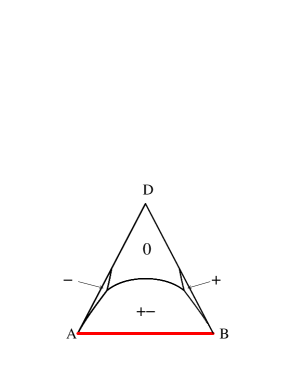
Figure 5: Exact phase diagram in the composition triangle $ABD$ of Fig. 2. The triple points, where the final state probabilities of three of the four phases are equal, are located at $(x,y)\approx(0.0507,0.6185)$ and $(x,y)\approx(0.6185,0.0507)$.

From our results for $P_{+-}(x,y)$, $P_{+}(x,y)$, $P_{-}(x,y)$, and $P_{0}(x,y)$, we may define a “phase diagram” shown in figure 5. Each region in the figure corresponds to the portion of the composition triangle where the probability of ultimately ending up in the labeled state is greater than all other first-passage probabilities. The least likely outcome is the achievement of extremist consensus while the most likely result is to get stuck in the frozen mixed state.

V MEAN EXIT TIME

In addition to the probability of reaching a particular final state, we also study the mean time until the final state is reached as a function of the initial composition of the system. The simplest such quantity is the unconditional mean time $t(x,y)$ to reach any of the four possible final states — extremist consensus ($+$ or $-$), centrist consensus, and mixed frozen state, as a function of the initial densities $x$ and $y$. This first-passage time can again be obtained trivially by considering an equivalent two-state system where we lump leftists and rightists into a single extremist state. The system stops evolving when the density of centrists reaches $z=0$ or $z=1$, with the former corresponding either to extremist consensus or to a frozen mixed state.

To find this first-passage time to reach the final state, note that in a single event the effective one-dimensional random walk that corresponds to the state of the system can either jump to one of its two nearest neighbors with probability $p_{z}$ or stay at the same site with probability $1-2p_{z}$, where $p_{z}=p_{x}+p_{y}=z(x+y)=z(1-z)$. The time interval for each event is $dt=1/N$, corresponding to each person being selected once on average every $N$ update steps. Then the mean time to reach the final states $z=0$ or $z=1$ as a function of the initial density $z$ obeys the recursion redner

$$t(z) = p_{z}[t(z+\delta)+dt]+p_{z}[t(z-\delta)+dt]$$ (24)

$$+ (1-2p_{z})[t(z)+dt].$$ (25)

This formula has a similar form and a similar explanation as the equation for the first-passage probability [Eq. (2)]. Starting from $z$, the mean time to reach the final state equals the probability of taking a single step (the factors $p_{z}$ and $1-2p_{z}$) multiplied by the time needed to reach the boundaries via this intermediate site. This path-specific time is just the mean first-passage time from the intermediate site plus the time $dt$ for the initial step.

In the large-$N$ limit this recursion reduces to

$$\frac{d^{2}t(z)}{dz^{2}}=-\frac{1}{D},$$ (26)

where the diffusion coefficient is $D={p_{z}}\delta^{2}/dt$. Since $dt=\delta=1/N$, we have $D=z(1-z)/N$. Eq. (26) is subject to the boundary conditions $t(0)=t(1)=0$, corresponding to immediate absorption if the random walk starts at the boundary. The solution to this equation is

$$t(z)=-N\left[z\;\ln z+(1-z)\;\ln(1-z)\right].$$ (27)

This is simply the mean consensus time of the 2-state voter model in the mean-field limit, in which the initial density of the two species are $z$ and $1-z$.

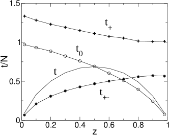
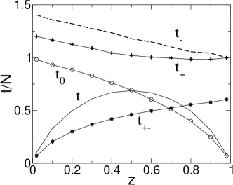
Figure 6: Unconditional and conditional exit times as a function of $z$ for the cases $y/x=1$ (top) and $y/x=2$ (bottom). The curves for $t$ and $t_{0}$ are based on exact formulae, while the other are based on simulations. The latter results are based on $10^{5}$ realizations for each initial state.

It is more interesting to consider the conditional first-passage time to a specific final state as a function of the initial condition. For example, consider the conditional time $t_{0}(z)$, the mean time to reach centrist consensus when the initial centrist density is $z$. This is the mean time for the equivalent random walk to hit the point $z=1$, without hitting $z=0$. In the large $N$ limit, this conditional exit time obeys the differential equation (see Sec. 1.6 in redner )

$$D\frac{d^{2}}{dz^{2}}[P_{0}(z)\;t_{0}(z)]=-P_{0}(z).$$ (28)

Integrating Eq. (28), using $P_{0}(z)=z$, and the boundary conditions $P_{0}(z)\;t_{0}(z)=0$ at $z=0$ and at $z=1$, we obtain $P_{0}(z)\;t_{0}(z)=-N\;(1-z)\;\ln(1-z)$, from which the conditional time to reach centrist consensus is

$$t_{0}(z)=-N\,\frac{1-z}{z}\;\ln(1-z).$$ (29)

Similarly, the mean time to reach all other final states of the system is

$$t_{\rm other}(z)=-N\,\frac{z}{1-z}\;\ln z.$$ (30)

In principle, we can find the conditional times to reach the extremist consensus states and the frozen final state as a function of the initial condition. This involves solving the two-dimensional analogue of Eq. (28) in the density triangle, subject to the appropriate boundary conditions. Because of the tedious nature of the calculation, we have instead resorted to numerical simulations to compute these conditional exit times. These results are shown in Fig. 6. While all exit times are of the order of $N$, it is worth noting that $t_{+}$ and $t_{-}$ are typically the longest times. This stems from the fact that reaching extremist consensus is a two-stage process. First, the extremists of the opposite persuasion must be eliminated, and then there is a subsequent first-passage process in which the centrists are also eliminated.

VI Discussion

We determined basic properties of the final state in a simple opinion dynamics model that consists of a population of leftists, rightists, and centrists. Centrists interact freely with extremists (either leftist or rightist), so that one agent adopts the opinion of its interaction partner, while extremists of opposite persuasions do not interact. These competing tendencies lead either to ultimate consensus or to a frozen final state that consists of non-interacting leftists and rightists. While this model is clearly an oversimplification of opinion evolution in a real population, it provides a minimalist description for how consensus or distinct cultural domains can be achieved.

Our calculations are based on the mean-field limit in which each individual interacts with any other individual with equal probability. It is worth emphasizing that the dependence of the final state probabilities on the initial composition of the population is very close to the corresponding quantities on finite-dimensional systems VKR . This coincidence is a reflection of the conservation of the global magnetization by the dynamics. Indeed, for the classical voter model, the conservation of the magnetization immediately leads to the fact that the probability of $+$ consensus is equal to the initial density of $+$ spins in any dimension.

There are two extensions of the model that are worth mentioning. First, it is natural that extremists have a stronger conviction than centrists. This suggests the generalization where a centrist adopts an extremist’s opinion with probability $p>1/2$ while an extremist adopts a centrist’s opinion with probability $q=1-p$ in an elementary update step. For this generalization, the densities of each species evolve by the following rate equations in the mean-field limit

$$\dot{x} = v\,z\,x$$

$$\dot{y} = v\,z\,y$$

$$\dot{z} = -v\,z\,(x+y)$$

where $v=p-q$ quantifies the bias. For $p\neq q$, The solution to these equations are

$$x(t)=\frac{x(0)\;e^{vt}}{1+[x(0)+y(0)](e^{vt}-1)},$$

and similarly for $y(t)$, while $z(t)=1-x(t)-y(t)$. In the long time limit and for $p>q$, we find

$$x\rightarrow\frac{x(0)}{x(0)+y(0)},\qquad y\rightarrow\frac{y(0)}{x(0)+y(0)},$$

while $z\rightarrow 0$. Thus if there is an innate bias favoring extremism, a frozen final state with no consensus is inevitable. On the other hand, if centrists are dominant ($p<q$), there centrist consensus is the final result.

Our results can also be adapted to determine the final states probabilities in the mean-field limit of the Axelrod model for the case of two features and two states per feature. The four possible states of an individual can be represented by

$$++\qquad--\qquad+-\qquad-+\;.$$

We define the dynamics to be that if an interaction pair has one common feature, then the other feature where disagreement exists is picked and the initial agent takes on the state of the interaction partner.

There are four possible consensus states: all $--$, $-+$, $+-$, and $++$, and two types of frozen states: mixtures of $--$ and $++$, and mixtures of $-+$ and $+-$. We can identify the states $--$ and $++$ in this Axelrod model with the $-$ and $+$ states, respectively, in our spin-1 Ising model, and the states $-+$ and $+-$ taken together with the 0 state of the spin-1 Ising model. Then, using our previous results, if the initial densities of $--$ and $++$ states are $x$ and $y$ respectively, the probabilities of $--$ and $++$ consensus and the probability of frozen mixture of $--$ and $++$ are given by the expressions $P_{-}(x,y)$, $P_{+}(x,y)$ and $P_{+-}(x,y)$ respectively (Eqs. (22) and (13)). By similar arguments, the probabilities of $-+$ and $+-$ consensus and the probability of $-+$ and $+-$ frozen mixture are given by the above expressions where $x$ and $y$ are now the initial densities of $-+$ and $+-$ states respectively. Unfortunately, this exact mapping onto an equivalent Ising spin system does not work when there are more than two features and/or more than two states per feature.

VII Acknowledgments

We thank Paul Krapivsky for useful discussions and helpful advice. We also thank NSF grant DMR0227670 for financial support of this research.

Appendix A Solution to Equivalent Schrödinger Equation

We present the solution to Eq. (11). This turns out be the Schrödinger equation for the Pöschl-Teller potential hole QM-book , for which the generic form of the equation is

$$\frac{d^{2}u(\theta)}{d\theta^{2}}+\left[k^{2}-\alpha^{2}\left(\frac{\chi(\chi-1)}{\sin^{2}\alpha\theta}+\frac{\lambda(1-\lambda)}{\cos^{2}\lambda\theta}\right)\right]u(\theta)=0,$$ (31)

with $k^{2}=1+m^{2}$, $\alpha=1$, $\chi=\lambda$, and $\chi(\chi-1)=3/4$. This last equation has the roots $\chi_{1}=3/2$ and $\chi_{2}=-1/2$. The eigenvalues and eigenvectors of Eq. (31) are (see, for example, QM-book page 92):

$$k^{2} = \alpha^{2}(\chi+\lambda+2n)^{2}$$

$$u_{n}(\theta) = \sin^{\chi}\alpha\theta\,\cos^{\lambda}\alpha\theta\;_{2}F_{1}(-n,\chi+\lambda+n,\chi+\frac{1}{2};\sin^{2}\alpha\theta),$$

with $n=0,1,2,..$, and where ${}_{2}F_{1}$ is the hypergeometric function.

For $\chi=-1/2$, $u_{n}(\theta)$ diverges at $\theta=0$ and $\theta=\pi/2$. Thus we take the solution for $\chi=3/2$ only and obtain the eigenfunctions and eigenvectors of Eq. (11):

$$1+m^{2} = (3+2n)^{2}$$ (32)

$$u_{n}(\theta) = \sin^{\frac{3}{2}}\theta\,\cos^{\frac{3}{2}}\theta\,\,\,_{2}F_{1}(-n,3+n,2;\sin^{2}\theta).$$

The solutions for the angular function in Eq. (7) therefore have the form

$$\Theta_{n}(\theta)=f(\theta)\,u_{n}(\theta)=\sin^{2}2\theta\,\,_{2}F_{1}(-n,3+n,2;\sin^{2}\theta),$$

with $m$ given by Eq. (32). Finally, the generic form of the product solution $F_{n}(\rho,\theta)=R_{n}(\rho)\,\Theta_{n}(\theta)$ to Eq. (5) is

$$F_{n}(\rho,\theta)=\left(A_{+}\rho^{2(2+n)}+A_{-}\rho^{-2(1+n)}\right)\Theta_{n}(\theta).$$

The coefficient $A_{-}$ must be zero because $F$ is zero at the origin. Thus

$$F_{n}(\rho,\theta)=\rho^{2(2+n)}\sin^{2}(2\theta)\,\,_{2}F_{1}(-n,3+n,2;\sin^{2}\theta),$$

and the general solution to Eq. (5) is

$$F(\rho,\theta)=\sum_{n=0}^{\infty}c_{n}\;\rho^{2(2+n)}\;\sin^{2}2\theta\,\,_{2}F_{1}(-n,3+n,2;\sin^{2}\theta).$$ (33)

We need the set of hypergeometric functions ${}_{2}F_{1}$ to form an orthogonal set to obtain the coefficients $c_{n}$ from the boundary condition:

$$F(\rho=1,\theta)=1=\sum_{n=0}^{\infty}c_{n}\;\sin^{2}2\theta\,\,_{2}F_{1}(-n,3+n,2;\sin^{2}\theta).$$

Fortunately, the functions ${}_{2}F_{1}$ are related, for certain specific integer parameters, to the Associated Legendre Polynomials (that are known to form an orthogonal set) via Grad :

$$P_{\nu}^{m}(x)=\frac{(-1)^{m}\;\Gamma(\nu+m+1)\;(1-x^{2})^{m/2}}{2^{m}\;\Gamma(\nu-m+1)\;m!}\;_{2}F_{1}(m-\nu,m+\nu+1;m+1;\frac{1-x}{2}).$$

If we take $m=1$, $\nu=n+1$ and $x=\cos 2\theta$ we obtain:

$${}_{2}F_{1}(-n,n+3;2;\sin^{2}\theta)=\frac{-2n!}{(n+2)!\;\sin 2\theta}\;P_{n+1}^{1}(\cos 2\theta).$$

Then the general solution Eq. (33) can be written as

$$F(\rho,\theta)=\sum_{n=0}^{\infty}c_{n}\;\rho^{2(2+n)}\;\sin 2\theta\,\,P_{n+1}^{1}(\cos 2\theta),$$ (34)

where we absorbed the factor $\frac{-2n!}{(n+2)!}$ into the coefficient $c_{n}$.

A.1 Solution for $P_{+-}$

To determine $P_{+-}$, we now apply the boundary condition $F=1$ at $\rho=1$ and obtain

$$F(\rho=1,\theta)=1=\sum_{n=0}^{\infty}c_{n}\;\sin 2\theta\,P_{n+1}^{1}(\cos 2\theta),$$

and using the orthogonality-normalization of the $P_{n}^{1}$’s we obtain the $c_{n}$’s:

$$c_{n}=\left\{\begin{array}[]{ll}{\displaystyle 0}&\mbox{~{}~{}~{}~{}~{} $n$ odd},\\ {\displaystyle\frac{(2n+3)}{(n+2)(n+1)}}&\mbox{~{}~{}~{}~{}~{} $n$ even},\end{array}\right.$$ (37)

Substituting these coefficients in Eq. (34), we obtain Eq. (III).

A.2 Solution for $P_{+}$

To determine $P_{+}$, we first need the first-passage probability $F(x^{\prime}|x,y)$ for the effective random walker to hit the specific point $(x^{\prime},1-x^{\prime})$ on the locus $x+y=1$, when starting from $(x,y)$. This first-passage probability also satisfies the basic differential equation (3), but with the boundary conditions given in Eq. (IV). In polar coordinates the last of these boundary conditions is $F(x^{\prime}|x,1-x)=F(\theta^{\prime}|\rho=1,\theta)=\delta(\cos^{2}\theta-\cos^{2}\theta^{\prime})$. Thus we now determine the coefficients $c_{n}$ in Eq. (34) by

$$\delta(\cos^{2}\theta-\cos^{2}\theta^{\prime})=\sum_{n=0}^{\infty}c_{n}\;\sin(2\theta)\,\,P_{n+1}^{1}(\cos 2\theta).$$

Inverting this relation and using the orthogonality of the $P_{n}^{1}$’s [Eq. (37)], we obtain

$$c_{n}=\frac{(2n+3)}{(n+2)(n+1)}\frac{P_{n+1}^{1}(\cos 2\theta^{\prime})}{\sin 2\theta^{\prime}}.$$

Using this result and transforming back to $xy$ coordinates, we obtain the first-passage probability

$$F(x^{\prime}|x,y)=\sum_{n=1}^{\infty}\frac{(2n+1)}{n(n+1)}\,\frac{P_{n}^{1}(2x^{\prime}-1)}{\sqrt{x^{\prime}(1-x^{\prime})}}\times\sqrt{xy}\,(x+y)^{n}\,P_{n}^{1}\left(\frac{x-y}{x+y}\right).$$ (38)

We then substitute this expression for $F(x^{\prime}|x,y)$ into Eq. (20) to determine $P_{+}(x,y)$. In so doing, we encounter the integral

$$I=\int_{0}^{1}x^{\prime}\frac{P_{n}^{1}(2x^{\prime}-1)}{\sqrt{x^{\prime}(1-x^{\prime})}}dx^{\prime}.$$

To evaluate this integral, we first make the variable change $x=2x^{\prime}-1$, use the identity $P_{n}^{1}(x)=\sqrt{1-x^{2}}\;\frac{dP_{n}(x)}{dx}$, and integrate by parts to give

$$I = \int_{-1}^{1}\frac{(x+1)}{2}\,\frac{P_{n}^{1}(x)}{\sqrt{1-x^{2}}}\,dx=\int_{-1}^{1}\frac{(x+1)}{2}\,\frac{dP_{n}(x)}{dx}\,dx,$$ (39)

$$= \left.\frac{(x+1)}{2}P_{n}(x)\right|_{-1}^{1}-1/2\int_{-1}^{1}P_{n}(x)\,dx,$$

$$= P_{n}(1)-\frac{1}{2}\int_{-1}^{1}P_{0}(x)P_{n}(x)\,dx=1-\delta_{n0},$$

where we have used $P_{0}(x)=1$, $P_{n}(1)=1\;\;\forall n$, as well as

$$\int_{-1}^{1}P_{m}(x)\,P_{n}(x)\,dx=\frac{2}{2n+1}\,\delta_{mn}.$$

Using the results of Eq. (38) and Eq. (39) in Eq. (20), we obtain the solution quoted in (22).

Appendix B Reduction of $P_{+-}$

To reduce the series representation (13) for $P_{+-}$ to a closed form, we start with the identity

$$P_{n}^{1}(0)=\left\{\begin{array}[]{ll}{\displaystyle 0}&\mbox{$n$ even},\\ {\displaystyle\frac{(-1)^{\frac{n-1}{2}}n!!}{(n-1)!!}}&\mbox{$n$ odd},\end{array}\right.$$

and make the variable change $n=2m+1$ with $m\geq 0$ integer to obtain

$$P_{+-}(z)=\sum_{m=0}^{\infty}\frac{(-1)^{m}\,(4m+3)\;(2m-1)!!}{2(m+1)(2m)!!}\;(1-z)^{2(m+1)}.$$ (40)

This infinite series can be summed by the following algebraic manipulation. We define $w=(1-z)^{2}$. The factor $4m+3$ can be rewritten as $(2m+1)+2(m+1)$, so that Eq. (40) becomes

$$P_{+-}(z) = \sum_{m=0}^{\infty}\frac{(-1)^{m}\,(2m+1)\;(2m-1)!!}{2(m+1)(2m)!!}\;w^{(m+1)}+\sum_{m=0}^{\infty}\frac{(-1)^{m}\,2(m+1)\;(2m-1)!!}{2(m+1)(2m)!!}\;w^{(m+1)},$$

$$= -\sum_{m=1}^{\infty}\frac{(2m-1)!!}{(2m)!!}\;(-w)^{m}+w\sum_{m=0}^{\infty}\frac{(2m-1)!!}{(2m)!!}\;(-w)^{m},$$

$$= 1-(1-w)\sum_{m=0}^{\infty}\frac{(2m-1)!!}{(2m)!!}\;(-w)^{m},$$

$$= 1-\frac{1-w}{\sqrt{1+w}},$$

where we used the Taylor series expansion

$$\frac{1}{\sqrt{1-x}}=\sum_{m=0}^{\infty}\frac{(2m-1)!!}{(2m)!!}\;x^{m}.$$

This then gives closed expression for the probability of reaching the mixed state as a function of $z$ quoted in Eq. (III).

References

- (1) S. Galam, J. Stat. Phys. 61, 943 (1990); Physica A 238, 66 (1997).
- (2) B. Latané and A. Nowak, in Progress in Communication Science, pp. 43, eds. G. A. Barnett and F. J. Boster (1997).
- (3) W. Weidlich, Sociodynamics; A Systematic Approach to Mathematical Modelling in the Social Sciences (Harwood Academic Publishers, 2000).
- (4) K. Sznajd-Weron and J. Sznajd, Int. J. Mod. Phys. C 11, 1157 (2000).
- (5) P. L. Krapivsky and S. Redner, Phys. Rev. Lett. 90, 238701 (2003).
- (6) R. Axelrod, J. Conflict Resolution 41, 203 (1997); R. Axelrod, The Complexity of Cooperation, (Princeton University Press, Princeton, 1997).
- (7) C. Castellano, M. Marsili, and A. Vespignani, Phys. Rev. Lett. 85, 3536 (2000); D. Vilone, A. Vespignani, and C. Castellano, Eur. Phys. J. B 30, 399 (2002).
- (8) T. M. Liggett, Interacting Particle Systems (Springer-Verlag, New York, 1985).
- (9) G. Deffuant, D. Neau, F. Amblard and G. Weisbuch, Adv. Complex Syst. 3, 87 (2000); G. Weisbuch, G. Deffuant, F. Amblard, and J.-P. Nadal, Complexity 7, 2002; G. Deffuant, F. Amblard, G. Weisbuch and T. Faure, Journal of Artificial Societies and Social Simulations 5, issue 4, paper 1 (jasss.soc.surrey.ac.uk) (2002).
- (10) R. Hegselmann and U. Krause, Journal of Artificial Societies and Social Simulation 5, issue 3, paper 2 (jasss.soc.surrey.ac.uk) (2002) and Physica A, in press (2004).
- (11) E. Ben-Naim, P. L. Krapivsky, and S. Redner, Physica D 183, 190 (2003).
- (12) F. Vazquez, P. L. Krapivsky, and S. Redner, J. Phys. A 36, L61 (2003).
- (13) S. Redner, A Guide to First-Passage Processes, (Cambridge University Press, New York, 2001).
- (14) Siegfried Flügge (1994) Practical Quantum Mechanics, (Springer-Verlag, Berlin, 1994).
- (15) I. S. Gradshteyn and I. M. Ryzhik, Table of Integrals, Series and Products, (Academic Press, San Diego, 1980).
- (16) A similar ultimate outcome also occurs in a cyclic 4-state voter model; see L. Frachebourg, P. L. Krapivsky, and E. Ben-Naim, Phys. Rev. E 54, 6186 (1996).