Role of transverse excitations in the instability of
Bose-Einstein condensates moving in optical lattices

Abstract

The occurrence of energetic and dynamical instabilities in a Bose-Einstein condensate moving in a one-dimensional (1D) optical lattice is analyzed by means of the Gross-Pitaevskii theory. Results of full 3D calculations are compared with those of an effective 1D model, the nonpolynomial Schrödinger equation, pointing out the role played by transverse degrees of freedom. The instability thresholds are shown to be scarcely affected by transverse excitations, so that they can be accurately predicted by effective 1D models. Conversely, transverse excitations turn out to be important in characterizing the stability diagram and the occurrence of a complex radial dynamics above the threshold for dynamical instability. This analysis provides a realistic framework to discuss the dissipative dynamics observed in recent experiments.

I Introduction

The occurrence of energetic and dynamical instabilities in a Bose-Einstein condensate (BEC) that moves in a periodic (optical) potential is an interesting problem from the conceptual viewpoint, since it involves basic properties of superfluids. Experimentally the dissipative dynamics of BECs moving through optical lattices has been investigated both in the weak burger ; burger2 and tight-binding regimes cataliotti ; lens , and a number of papers have recently been published in connection with these and similar experiments morsch ; oberthaler ; smerzi ; menotti ; pethick ; wuniu ; adhikari ; nesi ; taylor .

From the theoretical side, systematic investigations of the stability regimes have been so far presented for strictly one-dimensional (1D) systems. For deep optical lattices (tight-binding limit) it has been argued that the major mechanism responsible for the superflow breakdown of a moving BEC is the onset of a dynamical (modulational) instability wuniu ; smerzi . This behavior has also been confirmed by direct integration of the 3D Gross-Pitaevskii (GP) equation in the same regime adhikari ; nesi , and well reproduces the experimental observations lens . Conversely, the opposite limit of shallow lattices has been the object of a stimulating debate and it has been suggested that the origin of the observed instability could have an energetic or dynamic character burger ; burger2 ; wuniu .

Here we present a general discussion of the energetic and dynamical instabilities within the GP theory. We make use of a 3D description that includes the radial degrees of freedom in order to provide a reliable framework for a comparison with current experiments. In Sec. II, we briefly summarize the formalism of the standard linear analysis within the GP theory. Then, in Secs. III and IV, we discuss in detail the case of a cylindrical condensate in a 1D optical lattice, for which one can use Bloch functions and rigorously define the concept of quasimomentum associated with the motion of the condensate in the lattice. For any given quasimomentum of the condensate, we calculate the excitation spectrum and the stability diagram by solving the equations of the linearized GP theory review . The same quantities are also calculated by means of an effective 1D model, known as nonpolynomial Schrödinger equation (NPSE) salasnich , which includes the transverse direction through a Gaussian ansatz for the radial shape of the order parameter, with a $z$- and $t$-dependent width. With respect to strictly 1D models, which rely on a suitable renormalization of the mean-field coupling constant, the NPSE has the advantage that the true 3D coupling constant $g=4\pi\hbar^{2}a/m$ can be used, thus allowing for a direct comparison with experiments. It turns out that this model gives accurate predictions for the instability thresholds, the latter being mainly determined by the dispersion of the lowest branch of excitations, with no radial nodes. Higher branches, with one or more radial nodes, that are included in the GP theory but not in the NPSE, are shown to be important in characterizing the number and the type of excitations that become unstable above the instability threshold. They also produce a significant change in the shape of the dynamically unstable regions above threshold.

Finally, in Sec. V, we perform a GP simulation for the elongated condensate of the experiments of Ref. burger . The results of the simulation are analyzed by using the spectra and the phase diagrams of the cylindrical condensate of Secs. III and IV. This analysis provides convincing evidence that the breakdown of superfluid flow observed in Ref. burger is associated with the onset of a dynamical instability, triggered by the resonant coupling of Bogoliubov phonon and antiphonon modes. The subsequent dynamics is shown to strongly involve radial motions.

II GP equation and linear analysis

The GP equation for the order parameter $\psi$ of $N$ condensed atoms of mass $m$ and scattering length $a$ is review

$$i\hbar\frac{\partial}{\partial t}\psi(\mathbf{x},t)=\biggl{[}-\frac{\hbar^{2}}{2m}\nabla^{2}+V(\mathbf{x})+g|\psi(\mathbf{x},t)|^{2}\biggr{]}\psi(\mathbf{x},t)\,,$$ (1)

where $g=4\pi\hbar^{2}a/m$. We will consider the case of condensates confined in a harmonic potential superimposed to a 1D periodic optical lattice, $V(\mathbf{x})=V_{\rm ho}(\mathbf{x})+V_{\rm L}(z)$.

Let $\psi_{0}({\bf x},t)=\phi_{0}({\bf x})\exp(-i\mu t/\hbar)$ be a solution of the stationary GP equation, having chemical potential $\mu$,

$$\biggl{[}-\frac{\hbar^{2}}{2m}\nabla^{2}+V(\mathbf{x})+g|\phi_{0}({\bf x})|^{2}\biggr{]}\phi_{0}({\bf x})=\mu\phi_{0}({\bf x})\,,$$ (2)

and normalized according to $\int\!d^{3}x\ |\phi_{0}({\bf x})|^{2}=N$. If the state $\phi_{0}$ is a local minimum of the energy functional

$$E[\phi_{0}]=\int\!d^{3}x\ \phi_{0}^{*}\left[-\frac{\hbar^{2}}{2m}\nabla^{2}+V-\mu\right]\phi_{0}+\frac{g}{2}|\phi_{0}|^{4}$$ (3)

the system is energetically stable. Energetic (Landau) instability sets in when this condition is no longer true, and there are some directions in the $\psi$ space along which it is possible to lower the energy. This happens, for instance, when a uniform condensate flows with velocity $v$ in presence of a static external potential; if $v$ is larger than the velocity of Bogoliubov’s sound, then the system can lower its energy by emitting phonons (Landau criterion of superfluidity landau ). Similar conditions can be found for an inhomogeneous condensate moving in an optical lattice above a certain critical velocity $v_{E}$.

The condition for energetic stability can be formally derived by considering small deviations from $\phi_{0}$ in the form

$$\psi({\bf x},t)=e^{\displaystyle i\mu t/\hbar}[\phi_{0}({\bf x})+\delta\phi({\bf x},t)]\,,$$ (4)

and expanding the energy functional up to the quadratic terms

$$E[\phi]=E[\phi_{0}]+\int\!d^{3}x\ \left({\delta\phi^{*},\delta\phi}\right)M\pmatrix{{\delta\phi}\cr{\delta\phi^{*}}\cr}\,,$$ (5)

where

$$M=\pmatrix{H_{0}+2g|\phi_{0}|^{2}&g\phi_{0}^{2}\cr g\phi_{0}^{*2}&H_{0}+2g|\phi_{0}|^{2}\cr}$$ (6)

and

$$H_{0}=\left[-\frac{\hbar^{2}}{2m}\nabla^{2}+V-\mu\right].$$ (7)

The onset of energetic (Landau) instability is thus signaled by the appearance of negative eigenvalues in the spectrum of the operator $M$.

A second type of instability is the dynamical (modulational) instability. This occurs when the frequency of some modes in the excitation spectrum has a nonzero imaginary part. Then the occupation of these modes grows exponentially in time and rapidly drives the system away from the steady state. The conditions for the onset of this instability can be obtained again by means of the expansion (4). When inserted into the GP equation (1) it yields the Bogoliubov equations

$$\sigma_{z}M\pmatrix{{\delta\phi}\cr{\delta\phi^{*}}\cr}=\hbar\omega\pmatrix{\delta\phi\cr\delta\phi^{*}\cr}$$ (8)

whose character is now determined by the operator $\sigma_{z}M$, with

$$\sigma_{z}\equiv\pmatrix{1&0\cr 0&-1\cr}.$$ (9)

Energetic and dynamical instabilities are therefore related to the spectral properties of the operator $M$ and $\sigma_{z}M$ wuniu ; castin . This has two important consequences: (i) when the system is energetically stable it is also dynamically stable; (ii) the energetic instability, which is related to the spectrum of $M$, cannot be revealed by a direct integration of the time-dependent GP equation (1), which is dissipationless and is governed by the spectrum of $\sigma_{z}M$.

III Spectrum of a cylindrical condensate in a lattice

In order to perform explicit calculations, let us consider the case of an infinite cylindrical condensate, which is radially confined by the harmonic potential $V_{\rm ho}(r)=(1/2)m\omega_{r}^{2}r^{2}$, and is subject to the periodic potential $V_{\rm L}(z)=sE_{R}\cos^{2}(q_{B}z)$. The Bragg wave vector $q_{B}=\pi/d$ is determined by the lattice spacing $d$. The quantity $E_{\rm R}\equiv\hbar^{2}q_{B}^{2}/2m$ is the recoil energy of an atom absorbing one lattice photon and $s$ is a dimensionless parameter fixing the lattice intensity. Such a cylindrical condensate is an accurate representation of an elongated axially symmetric condensate, when the weak axial harmonic confinement can be neglected. The major advantage of this geometry is that one can exploit the periodicity of the system by expanding the order parameter on a basis of Bloch functions, with the same period of the lattice.

III.1 Linearized GP equation

Within the GP theory, the starting point of the linear stability analysis for the cylindrical condensate is the expression

$$\psi(r,z,t)={\rm e}^{\displaystyle-i\mu_{p}t}{\rm e}^{\displaystyle ipz}\left[\phi_{p0}(r,z)+\delta\phi_{p}(r,z,t)\right]\,.$$ (10)

The Bloch wave vector $p$ (also called quasimomentum of the condensate) is associated with the velocity of the condensate in the lattice and is restricted to the first Brillouin zone wuniu ; menotti . For a given $p$, the function $\phi_{p0}$ is the solution of the stationary GP equation with energy $E_{p}$, while the excited part of the order parameter can be written as

$$\delta\phi_{p}(r,z,t) = \sum_{q,j}\left(u_{pq,j}(r,z){\rm e}^{\displaystyle i(qz-\omega_{pq,j}t)}\right.$$ (11)

$$\left.+v^{*}_{pq,j}(r,z){\rm e}^{\displaystyle-i(qz-\omega_{pq,j}t)}\right)\,,$$

where $q$ is the Bloch wave vector (or quasimomentum) of the excitations, and $j$ represents all possible values of the two quantum numbers $\alpha=1,2,3,\dots$ and $\nu=0,1,2,\dots$. The former is Bloch band index and the latter is the number of radial nodes in the Bogoliubov quasiparticle amplitudes $u$ and $v$. Along $z$ all the functions $\phi_{p0}$, $u_{pq,j}$ and $v_{pq,j}$ are periodic with the same period of the lattice.

Inserting the above expressions into the GP equation (1), one gets the Bogoliubov equations

$$\left[H_{r}+H_{z+}-\mu_{p}+2g|\phi_{p0}|^{2}\right]u+g\phi_{p0}^{2}v=\hbar\omega u$$ (12)

$$\left[H_{r}+H_{z-}-\mu_{p}+2g|\phi_{p0}|^{2}\right]v+g\phi_{p0}^{*2}u=-\hbar\omega v$$ (13)

with

$$H_{r} = -{\hbar^{2}\over 2m}\nabla_{r}^{2}+\frac{1}{2}m\omega_{r}^{2}r^{2}$$ (14)

$$H_{z\pm} = {\hbar^{2}(-i\partial_{z}\pm p+q)^{2}\over 2m}+sE_{R}\cos^{2}(q_{B}z)\,.$$ (15)

The quasiparticle amplitudes $u$ and $v$ satisfy the relation

$$\int\!d^{2}r\int^{d/2}_{-d/2}\!dz\ (u_{pq,i}u_{pq,j}^{*}-v_{pq,i}v_{pq,j}^{*})=\delta_{ij}\,.$$ (16)

Note that, for each quasiparticle obeying this orthonormality conditions, the Bogoliubov equations admit an antiquasiparticle with norm $-1$, which corresponds to replacing the amplitudes $(u,v)$ with $(v^{*},u^{*})$ wuniu ; castin .

The above equations can be solved numerically. We choose the relevant parameters such to simulate typical elongated condensates of the experiments of Ref. burger . The linear atomic density in the $z$ direction, averaged over the lattice length $d$, is taken to be equal to the linear density of the actual 3D condensate, close to the trap center and in the absence of the lattice. Here the chemical potential for $p=0$ is taken to be $\mu_{0}=7.2~{}\hbar\omega_{r}$. We also use $2\pi\ q_{B}^{-1}=800$ nm and $\omega_{r}=2\pi\times 90$ Hz. For each $p$, the order parameter $\phi_{p0}(r,z)$ and its energy $E_{p}$ are calculated by solving the stationary GP equation by means of iterative methods. Then the Bogoliubov equations (12) and (13) are transformed into matrix equations by projecting the functions $u$ and $v$ on the Bessel-Fourier basis $|l,n\rangle\equiv J_{0}\left({\alpha_{0n}r}/{r_{max}}\right)\exp(i2q_{B}lz)$, where $\alpha_{0n}$ are zeros of the Bessel functions $J_{0}(r)$ and $r_{max}$ is the radius of the computational box tozzo ; iyanaga . The resulting equations are not diagonal over the Fourier index $l$, and involve the numerical diagonalization of a $2\times N_{r}\times N_{z}$ rank matrix.

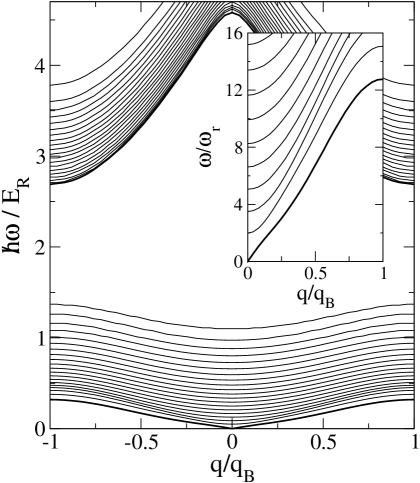
Figure 1: Excitation spectrum of a cylindrical condensate at rest in the optical lattice (quasimomentum of the condensate $p=0$) as a function of the quasimomentum $q$ of the excitations, for lattice intensity $s=5$. The first two Bloch bands are shown and for each band we plot the first $20$ radial branches. The lowest branch in each band (thickest line) corresponds to axial excitations with no radial nodes. In the inset we show a magnification of the low energy spectrum.

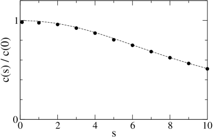
Figure 2: Bogoliubov sound velocity $c$ as a function of the lattice intensity $s$. Points: slope of the lowest phononic branch in the Bogoliubov spectrum of the cylindrical condensate. Dashed line: analytic prediction $c=(\kappa m^{*})^{-1/2}$ (see text).

The $p=0$ case corresponds to the condensate at rest. In Fig. 1 we show a typical spectrum, for $s=5$. The first two Bloch bands ($\alpha=1$ and $2$) are shown. For each band, we plot the first $20$ radial branches ($\nu=0,1,2,\dots,19$). The thickest lines are the dispersion laws of the $\nu=0$ excitations. A magnification of the low-energy branches is shown in the inset. The lowest branch corresponds to the dispersion law of $\nu=0$ axial phonons. It starts linearly at $q\to 0$ and its slope is the Bogoliubov sound velocity $c$. We calculate the slope for different values of the lattice intensity $s$ and we plot the results in Fig. 2 (points). The dashed line is the analytic prediction $c=(m^{*}\kappa)^{-1/2}$ of Ref. meret , where the effective mass $m^{*}$ and the compressibility $\kappa$ are defined as $m^{*}=\lim_{p\to 0}(\partial^{2}E_{p}/\partial p^{2})^{-1}$ and $\kappa^{-1}=\bar{n}(\partial\mu/\partial\bar{n})$ (see also the discussion in Ref. taylor ). Here we calculate the effective mass from the numerical values of the energy $E_{p}$. The compressibility is taken to be the one of a uniform gas in the same 1D optical lattice and with density equal to the average density of the cylindrical condensate (for the radial average we use the Thomas-Fermi value $\bar{n}=n(0)/2$ where $n(0)$ is the central density). The agreement is remarkable. The value at $s=0$ is the sound velocity $c=[gn(0)/(2m)]^{1/2}$ in a cylindrical condensate without lattice zaremba . Finally, we note that the $\nu=1$ branch in the inset of Fig. 1 exactly starts at $\omega=2\omega_{r}$ for $q=0$, where it corresponds to the radial breathing mode of the cylindrical condensate.

At $p\neq 0$, when the condensate moves in the lattice, the whole spectrum changes. In Fig. 3 we show a sequence of six spectra for $s=5$ and $p/q_{B}=0,0.25,0.5,0.55,0.75,1$. The real part of the frequencies $\omega_{pq,j}$ is plotted. At $p=0$ quasiparticles and antiquasiparticles have the same energy, since the system is symmetric under $z\to-z$ inversion. For a given $q$, they correspond to excitations propagating in opposite directions (opposite sign of $\omega$). In Fig. 3 the spectrum of antiquasiparticles, at $p=0$, is plotted in the negative $\omega$ plane.

By increasing $p$, the slope of the $\nu=0$ phononic branch increases for phonons which propagate forwards on top of the traveling condensate. Vice versa it decreases for those propagating backwards and their dispersion law eventually crosses the $\omega=0$ axis and changes sign. By further increasing $p$, one notices that the frequency of both phonons and antiphonons approaches zero at the boundaries of the Brillouin zone. At a critical quasimomentum $p_{D}$ ($p_{D}=0.525~{}q_{B}$ in our case), the real part of the $\nu=0$ mode frequency vanishes at $q=\pm q_{B}$. Phonon and antiphonon pairs thus exhibit a resonance coupling by first-order Bragg scattering, giving rise to a dynamical instability. For 1D condensates this process has been already discussed in Ref. wuniu . The coupled pairs of excitations, with $|q|=q_{B}=\pi/d$, start having imaginary frequency. The system can therefore develop a macroscopic standing wave, whose wavelength is twice the lattice spacing, which implies an out-of-phase oscillation of the condensate population in adjacent lattice sites. This is also consistent with the results of the 1D simulations of Ref. menotti .

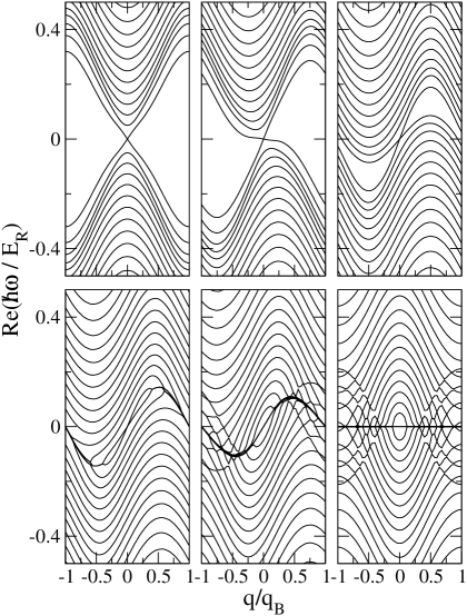
Figure 3: Real part of the excitation spectrum of a cylindrical condensate in a lattice with $s=5$ and for different values of the condensate quasimomentum $p$ ($p/q_{B}=0,0.25,0.5,0.55,0.75,1$), calculated from Eqs. (12)-(13).

For $p>p_{D}$ the coupling between $\nu=0$ phonons and antiphonons extends from zone boundary to lower values of $q$. Moreover, modes with radial nodes ($\nu>0$) also couple, first at $q=q_{B}$ and then down to lower $q$’s. A conjugate pair of complex frequencies appears each time a resonant coupling occurs between a pair of quasiparticle and antiquasiparticle that are degenerate prior to the coupling. An example is given in Fig. 4 where we plot the real and imaginary parts of the eigenfrequencies obtained by solving Eqs.(12) and (13) in the case $p/q_{B}=0.55$. Finally, as one can see in the last two frames of Fig. 3, a complicate sequence of no-crossing patterns also develop between modes belonging to the quasiparticle spectrum or between those belonging to the antiquasiparticle spectrum. These no-crossings do not produce any dynamical instability, but they contribute to mix up several radial branches via hybridization processes, which are not included in 1D models.

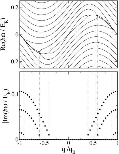
Figure 4: Real (top) and imaginary (bottom) parts of the frequencies obtained from Eqs. (12)-(13) for $s=5$ and $p/q_{B}=0.55$. The vertical (dotted) lines correspond to the points where a conjugate pair of complex frequencies appears.

III.2 Nonpolynomial Schrödinger equation

The description of the system can be simplified by using an effective 1D model, the nonpolynomial Schrödinger equation (NPSE) salasnich , which partially includes also the radial to axial coupling, and has been shown to provide a realistic description in several situations salasnich ; massignan ; nesi . This model is obtained from the GP equation by means of a factorization of the order parameter in the product of a Gaussian radial component of $z$- and $t$-dependent width, $\sigma(z,t)$, and of an axial wave function $\psi(z,t)$ that satisfies the differential equation

$$i\hbar\frac{\partial}{\partial t}\psi(z,t) = \bigg{[}-\frac{\hbar^{2}}{2m}\nabla_{z}^{2}+V(z)+\frac{gN}{2\pi\sigma^{2}}|\psi|^{2}$$

$$+\frac{1}{2}\hbar\omega_{r}\left(\frac{a_{r}^{2}}{\sigma^{2}}+\frac{\sigma^{2}}{a_{r}^{2}}\right)\bigg{]}\psi(z,t)\,,$$

coupled with an algebraic equation for the radial width

$$\sigma(z,t)=a_{r}\sqrt[4]{1+2aN|\psi(z,t)|^{2}}\,.$$ (18)

Here $a_{r}=\sqrt{\hbar/m\omega_{r}}$ is the radial oscillator length. By expanding $\psi(z,t)$ around the stationary wave function $\phi_{0}(z)$ and using Eqs. (III.2) and (18), it is straightforward to obtain the Bogoliubov-like equations

$$\pmatrix{H_{0}+A&B\cr-B^{*}&-(H_{0}+A)\cr}\pmatrix{\delta\phi\cr\delta\phi^{*}\cr}=\hbar\omega\pmatrix{\delta\phi\cr\delta\phi^{*}\cr}\,,$$ (19)

$$H_{0} = -\frac{\hbar^{2}}{2m}\nabla_{z}^{2}+V(z)$$ (20)

$$A = \frac{gN}{2\pi}\frac{|{\phi_{0}}|^{2}}{\sigma^{2}}\left(2-Na|\phi_{0}|^{2}\frac{a_{r}^{4}}{\sigma^{4}}\right)$$

$$+ \frac{1}{2}\hbar\omega_{r}\left[\frac{\sigma^{2}}{a_{r}^{2}}+\frac{a_{r}^{2}}{\sigma^{2}}+Na\phi_{0}^{2}\frac{a_{r}^{2}}{\sigma^{2}}\left(1-\frac{a_{r}^{4}}{\sigma^{4}}\right)\right]\,,$$

$$B = \frac{gN}{4\pi}\frac{{\phi_{0}}^{2}}{\sigma^{2}}\!\left[\frac{5}{2}-2Na|{\phi_{0}}|^{2}\frac{a_{r}^{2}}{\sigma^{2}}-\frac{1}{2}\frac{a_{r}^{4}}{\sigma^{4}}\right]\,.$$ (22)

The solution of these equations is obtained by a numerical matrix diagonalization. Compared to the solution of the Bogoliubov equations (12) and (13), the calculation of the spectrum from Eqs. (19) is much faster.

Owing to the partial coupling between axial and radial degrees of freedom, the NPSE provides a more accurate description of the actual 3D condensates with respect to strictly 1D models. An important advantage consists in the fact that, differently from strictly 1D models, the NPSE does not require any renormalization procedure for the coupling constant $g$, thus offering the possibility to make a direct comparison with experiments, as well as with GP calculations for 3D condensates. In this respect one has to remark also that, since the radial degrees of freedom are included through a single function $\sigma(z,t)$, the NPSE only accounts for $\nu=0$ radial excitations. The comparison between the predictions of the NPSE and those of the GP equation for the cylindrical condensate is thus particularly helpful to point out the role of the $\nu>0$ radial modes.

In Fig. 5 we plot the real (solid lines) and imaginary part (dashed lines) of the excitation frequencies obtained with the NPSE for the same $s$ and $p$ of Fig. 3. The two branches correspond to the $\nu=0$ phonon and antiphonon dispersions and their behavior is shown to closely follow that of the lowest $\nu=0$ branches of the GP case. In particular, the critical value $p=p_{D}$ at which the two modes couple at $q=q_{B}$, giving rise to dynamical instability, coincides with the GP result ($p_{D}=0.525~{}q_{B}$). The qualitative behavior is very similar also to that found in the 1D analysis of Ref. menotti .

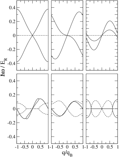
Figure 5: Excitation spectrum obtained from the NPSE for a cylindrical condensate in a lattice with $s=5$ and for different values of the quasimomentum $p$, as in Fig. 3 ($p/q_{B}=0,0.25,0.5,0.55,0.75,1$).

IV Stability diagrams

By repeating the calculations of the Bogoliubov frequencies (eigenvalues of the matrix $\sigma_{z}M$) for different values of the condensate quasimomentum $p$, one can draw the dynamically unstable regions in the $p$-$q$ plane. In the same way, one can find the spectrum of the matrix $M$ and draw the regions of energetic instability. The calculations can be performed both with GP theory and NPSE. Typical results are shown in Fig. 6 for $s=1,5,$ and $10$. The white area corresponds to a stable condensate; the light shaded area to a condensate which is energetically unstable (in the presence of dissipative processes, the energy can be lowered by emitting phonons of quasimomentum $q$ which lie in the shaded range); finally the dark shaded area is the region where the system is both energetically and dynamically unstable. The thresholds for energetic and dynamical instability correspond to the lowest values of $p$ at which the instability occurs. Let us call them $p_{E}$ and $p_{D}$, respectively.

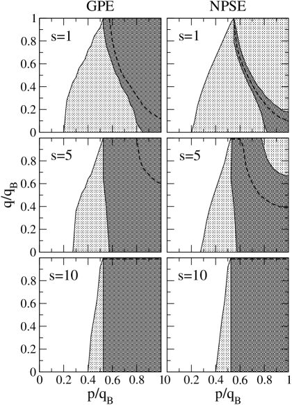
Figure 6: Stability diagrams obtained from the GP spectra (left) and NPSE spectra (right) as a function of the quasimomenta $p$ and $q$ of the condensate and of the quasiparticles, respectively, and for $s=1,5,10$. Shaded areas represent the regions where the system is dynamically (dark) and/or energetically (both light and dark) unstable. Dashed lines correspond to the modes having the largest imaginary part (most unstable modes).

Two main features emerge from the comparison of GP with NPSE: (i) the left border of the energetically and dynamically unstable regions are very similar in the two cases, which also implies a a good agreement for the critical quasimomenta $p_{E}$ and $p_{D}$; (ii) for small values of $s$ the shape of the dynamically unstable region above threshold looks rather different.

The first point is better visualized in Fig. 7, where we show the results for $p_{E}$ and $p_{D}$ as a function of $s$. The predictions of the two models are almost indistinguishable for both the energetic and dynamical instabilities in the whole range of $s$ here considered. These results confirm that the NPSE can be used as an efficient model to quantitatively identify the onset of instability for a wide range of $s$, relevant for available experiments nesi . The reason for its accuracy in predicting the thresholds is simply that the critical quasimomenta $p_{E}$ and $p_{D}$ are determined by the behavior of the $\nu=0$ branch of excitations with no radial nodes. A comparison between Figs. 3 and 5 shows that these modes are indeed very accurately described by the NPSE up to the instability threshold.

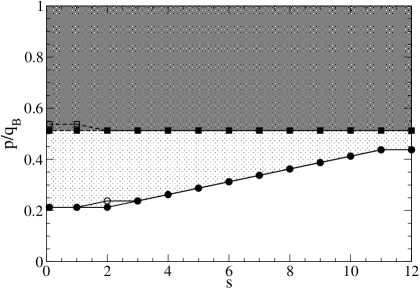
Figure 7: Thresholds for energetic (circles) and dynamical (squares) instability as a function of the lattice intensity $s$. The results of GP (filled symbols) and NPSE (empty symbols) are almost indistinguishable. Shaded areas represent the regions where the system is dynamically (dark) and/or energetically (both light and dark) unstable, according to the GP.

A closer inspection of the stability diagrams shows a difference in the shape and size of the dynamically unstable region at small $s$. The one predicted by NPSE does not fill the whole region above threshold. This agrees with previous 1D models wuniu ; menotti , but disagrees with the predictions of 3D GP equation. This disagreement can be easily understood by looking at the role played by the transverse degrees of freedom. In the NPSE, which only accounts for $\nu=0$ modes, nonvanishing complex frequencies appear when phonons and antiphonons couple, collapsing onto a single dispersion law. For a given $p$, this provides a range of $q$ for unstable modes, which starts first at $q_{B}$ and then lowers towards $q\to 0$ (see Fig. 5). However, at high enough $p$, the dispersion of the phonon-antiphonon pair splits again into two separate curves and this gives a window of stable modes from a certain $q$ (at fixed $p$) up to zone boundary. This window is the dynamically stable region on the top-right corner of the NPSE stability diagrams in Fig. 6. Now, by looking at the GP spectra in Fig. 3, one can easily understand why these stable regions are absent in the GP stability diagrams. The $\nu=0$ modes in this case are mixed up with several $\nu>0$ branches and these radial modes can be unstable also in the range of $q$ where the $\nu=0$ modes are stable. It is worth stressing that the occurrence of complex frequencies for such radial excitations also implies that, once the system is brought into the unstable region above $p_{D}$, it can easily develop macroscopic motions with a nontrivial radial dynamics.

Finally, it is interesting to compare the predictions of GP and NPSE for the growth rate, $|{\rm Im}(\omega)|$, of the most dynamically unstable modes. The results are shown in Fig. 8. At small $s$, the agreement between the two calculations (solid and empty symbols) is rather good. By increasing $s$ the agreement for the absolute values of growth rates becomes less and less quantitative. However, for each value of $s$, the shape of the GP and NPSE curves is still quite similar. This result is interesting in view of the comparison with experiments, where the shapes of these curves can be more relevant than their absolute values. In the experiments, in fact, it is much more likely to measure loss rates (or lifetimes) on large timescales, and estimate their relative increase as a function of $p$, rather than the absolute values of the growth rates in the small amplitude linear regime (short times).

Figure 8: Growth rates of the most dynamically unstable modes for different values of the lattice intensity $s$ ($s=0.1$ triangles, $s=1$ squares, $s=5$ circles) obtained with both GP and NPSE (filled and empty symbols, respectively).

V An experiment revisited

In this section we compare the predictions of the linear analysis discussed so far with the direct solutions of the time-dependent Gross-Pitaevskii equation (1). As an example we consider the case of the LENS experiment presented in Ref. burger , which has been the object of a stimulating debate on the origin of the observed instability burger2 . Indeed two interesting questions have been raised: (i) whether the GP equation is suitable to describe the phenomenology observed in the experiment, and (ii) whether the observed breakdown of superfluid flow comes from energetic and/or dynamical instability.

To model the LENS experiment burger , we consider an elongated ${}^{87}\mathrm{Rb}$ condensate with $N=3\times 10^{5}$ atoms confined in an axially symmetric harmonic trap of frequencies $\omega_{r}=2\pi\times 90$ Hz, $\omega_{z}=2\pi\times 8.7$ Hz. The optical lattice along $z$ is produced with laser beams of wavelength $\lambda=2\pi/q_{B}=795$ nm and intensity $s=1.59$. The system is prepared in the ground state of the combined harmonic+periodic potential and then is let evolve after a sudden displacement $\Delta z$ of the harmonic trapping.

If one considers not too large displacements the evolution of the condensate wave function can be safely described by a state of well defined quasimomentum (before instabilities occur) nesi . Using the formalism of Secs. III and IV we first calculate the stability diagram predicted by the linearized GP theory for an infinite cylinder having the same linear density as the one of the actual 3D elongated condensate near its center. The diagram is plotted in the upper part of Fig. 9. In the lower part we show the center-of-mass velocity, defined as $v_{\rm cm}=\partial E_{p}/\partial p$, obtained by solving the stationary GP equation (solid line). The two horizontal dotted lines indicate the critical velocities for the onset of energetic ($v_{E}$) and dynamical ($v_{D}$) instability.

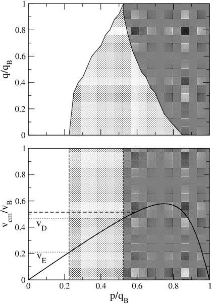
Figure 9: Top: GP stability diagram for a cylindrical condensate which approximates the experimental elongated condensate of Ref. burger in its central region. Light and dark shaded areas are unstable regions, as in Fig. 6. Bottom: center-of-mass velocity as a function of the condensate quasimomentum ($v_{B}=\hbar q_{B}/m$). The critical velocities for the energetic ($v_{E}$) and dynamical ($v_{D}$) instabilities of the cylindrical condensate are shown as horizontal dotted lines. The horizontal dashed line is the velocity at which the instability occurs in the GP simulation of the experimental 3D condensate of Ref. burger .

Then we numerically integrate the full 3D GP equation, using the experimental parameters. The evolution of the condensate and of its center-of-mass velocity, after an initial lateral displacement of $60$ $\mu$m, is shown in Fig. 10. As the figure shows, the condensate first accelerates towards the new trap center (to the left in the insets) by keeping its shape. The overall phase of the order parameter is also preserved, except for the addition of the extra phase associated with the translational motion. At a critical velocity the coherence is suddenly lost and the order parameter develops a complex structure, starting from its center. This critical velocity is also shown in the lower part of Fig. 9 (horizontal dashed line). It turns out to be very close to the one predicted for dynamical instability of the cylindrical condensate and well above the threshold of energetic instability. Finally, the critical velocity found in our GP simulations nicely agrees with the velocity at which the breakdown of superfluidity was observed in Ref. burger ($\simeq 0.5v_{B}$), therefore confirming that the dynamical instability plays a major role in this kind of experiments, as previously argued by Wu and Niu wuniu .

Figure 10: Center-of-mass velocity of the condensate during the its evolution in the harmonic trap after an initial displacement of $60$ $\mu$m. The velocity initially increases, as expected for the harmonic dipole oscillation of the whole condensate, up to a critical value at which the condensate breaks up. The corresponding quasimomentum $p$ lies in the dynamical unstable region of Fig. 9. In the insets we plot the linear density of the condensate along $z$ at different times. The horizontal ruler has a width of $280~{}\mu$m and the center of the trap is at mid point.

The GP simulation also reproduces the shape of the density distribution after the onset of the instability (see insets of Fig. 10 and the density plots in Fig. 11) which is characterized by a condensed/coherent part plus a broader incoherent distribution on the right side, as observed in the experiment burger . The instability starts close to the center of the condensate. Radial excitations are involved in this process, as can be deduced by the occurrence of density patterns with radial nodes.

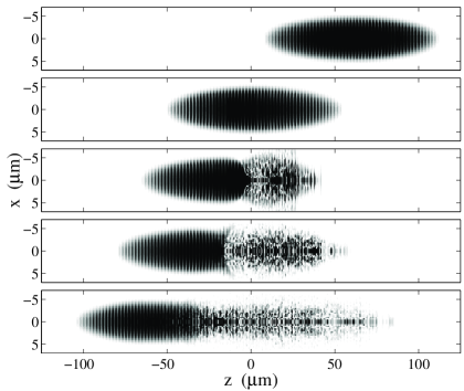
Figure 11: Density plots in the $(z,x)$ plane for different evolution times, corresponding to the inset pictures of Fig. 10 ($t=0,~{}30,~{}35,~{}40,~{}50$ ms), after an initial displacement $\Delta z=60$ $\mu$m. The parameters are those of the experiment in Ref. burger .

By repeating the same simulations for much larger initial displacements we find that the system can enter well inside the dynamically unstable region before decoherence processes take place. In this case, the acceleration of the condensate is so fast that dynamically unstable modes have not enough time to grow in a significant way. Eventually, for very large displacements the condensate passes through the entire dynamically unstable region and reaches the zone boundary, at $p\sim q_{B}$. At this point, the whole condensate undergoes a Bragg reflection soon followed by a sudden disruption process, involving solitons and vortex rings. This agrees with the recent GP simulations of Ref. scott , where the value $\Delta z=150~{}\mu$m has been used and the nature of this instability has been discussed in detail.

VI Conclusions

A general discussion of energetic and dynamical instabilities of a Bose-Einstein condensate moving in a 1D optical lattice has been presented using the Gross-Pitaevskii theory. We have shown that transverse excitations are important in characterizing the stability diagram and the occurrence of a complex radial dynamics above the threshold for dynamical instability.

The results of the full 3D calculations have been compared with those of an effective 1D model, the nonpolynomial Schrödinger equation (NPSE), which includes the effects of the transverse direction through a Gaussian ansatz for the radial component of the order parameter salasnich . This model is shown to give accurate predictions for the instability thresholds, that are mainly determined by the dispersion of the lowest branch of excitations, with no radial nodes.

The linear response analysis, in combination with the direct solution of the time-dependent GP equation, provides a realistic framework to discuss the dissipative dynamics observed in recent experiments. As an example here we have considered the case of experiments of Ref. burger , providing a convincing evidence that the observed breakdown of superfluid flow is associated with the onset of a dynamical instability.

The present analysis is also relevant in connection with the more recent experiments of Ref. fallani where the condensate is loaded adiabatically in a moving lattice. In this case, interesting results have been found by comparing the NPSE results with the experimental data for the nontrivial dissipative behavior of condensates loaded in higher Bloch bands fallani . In this respect, our work provides a further useful information, by pointing out in which cases, and for which observables, the NPSE is a reliable approximation of the full GP theory.

- (1) S. Burger, F. S. Cataliotti, C. Fort, F. Minardi and M. Inguscio, M. L. Chiofalo and M. P. Tosi, Phys. Rev. Lett. 86, 4447 (2001).
- (2) B. Wu and Q. Niu, Phys. Rev. Lett. 89, 088901 (2002); S. Burger et al., ibid. 89, 088902 (2002).
- (3) F. S. Cataliotti, S. Burger, C. Fort, P. Maddaloni, F. Minardi, A. Trombettoni, A. Smerzi, and M. Inguscio, Science 293, 843 (2001).
- (4) F. S. Cataliotti, L. Fallani, F. Ferlaino, C. Fort, P. Maddaloni, and M. Inguscio, New J. Phys. 5, 71 (2003).
- (5) M. Cristiani, O. Morsch, N. Malossi, M. Jona-Lasinio, M. Anderlini, E. Courtade, and E. Arimondo, Opt. Express 12, 4 (2004).
- (6) T. Anker, M. Albiez, B. Eiermann, M. Taglieber, and M. K. Oberthaler, Opt. Express 12, 11 (2004).
- (7) B. Wu and Q. Niu, Phys. Rev. A 64, 061603 (2001); New J. Phys. 5, 104 (2003).
- (8) A. Smerzi, A. Trombettoni, P. G. Kevrekidis, and A. R. Bishop, Phys. Rev. Lett 89, 170402 (2002).
- (9) C. Menotti, A. Smerzi, and A. Trombettoni, New J. Phys. 5, 112 (2003).
- (10) M. Machholm, C. J. Pethick, and H. Smith, Phys. Rev. A 67, 053613 (2003); M. Machholm, A. Nicolin, C. J. Pethick, and H. Smith, ibid. 69, 043604 (2004).
- (11) S. K. Adhikari, Eur. Phys. J. D 25, 161 (2003); J. Phys. B: At. Mol. Opt. Phys. 36, 3951 (2003).
- (12) F. Nesi and M. Modugno, J. Phys. B: At. Mol. Opt. Phys 37, S101 (2004).
- (13) E. Taylor and E. Zaremba, Phys. Rev. A 68, 053611 (2003).
- (14) F. Dalfovo, S. Giorgini, L. P. Pitaevskii, and S. Stringari, Rev. Mod. Phys. 71, 463 (1999).
- (15) L. Salasnich, Laser Phys. 12, 198 (2002); L. Salasnich, A. Parola, and L. Reatto, Phys. Rev. A 65, 043614 (2002).
- (16) E.M Lifshitz and L.P. Pitaevskii, Statistical Physics (Pergamon Press, Oxford, 1980), Part 2, p. 88.
- (17) Y. Castin, in Coherent Atomic Matter Waves, edited by R. Kaiser, C. Westbrook, and F. David, Lecture Notes of Les Houches Summer School (EDP Sciences and Springer-Verlag, Heidelberg, 2001), pp. 1-136.
- (18) C. Tozzo and F. Dalfovo, New J. Phys. 5, 54 (2003).
- (19) S. Iyanaga and Y. Kawada, Encyclopedic Dictionary of Mathematics (MIT Press Cambridge, MA, 1977).
- (20) M. Krämer, C. Menotti, L. Pitaevskii, and S. Stringari, Eur. Phys. J. D 27, 247 (2003).
- (21) E. Zaremba, Phys. Rev. A 57, 518 (1998); S. Stringari, ibid. 58, 2385 (1998).
- (22) P. Massignan and M. Modugno, Phys. Rev. A 67, 023614 (2003).
- (23) R. G. Scott et al., Phys. Rev. A 69, 033605 (2004).
- (24) L. Fallani et al., Phys. Rev. Lett. 93, 140406 (2004).