Poiseuille flow in a heated granular gas

Abstract

The planar Poiseuille flow induced by a constant external field (e.g., gravity) has been the subject of recent interest in the case of molecular gases. One of the predictions from kinetic theory (confirmed by computer simulations) has been that the temperature profile exhibits a bimodal shape with a local minimum in the middle of the slab surrounded by two symmetric maxima, in contrast to the unimodal shape expected from the Navier–Stokes (NS) equations. However, from a practical point of view, the interest of this non-Newtonian behavior in molecular gases is rather academic since it requires values of gravity extremely higher than the terrestrial one. On the other hand, gravity plays a relevant role in the case of granular gases due to the mesoscopic nature of the grains. In this paper we consider a dilute gas of inelastic hard spheres enclosed in a slab under the action of gravity along the longitudinal direction. In addition, the gas is subject to a white-noise stochastic force that mimics the effect of external vibrations customarily used in experiments to compensate for the collisional cooling. The system is described by means of a kinetic model of the inelastic Boltzmann equation and its steady-state solution is derived through second order in gravity. This solution differs from the NS description in that the hydrostatic pressure is not uniform, normal stress differences are present, a component of the heat flux normal to the thermal gradient exists, and the temperature profile includes a positive quadratic term. As in the elastic case, this new term is responsible for the bimodal shape of the temperature profile. The results show that, except for high inelasticities, the effect of inelasticity on the profiles is to slightly decrease the quantitative deviations from the NS results.

I Introduction

As is well known, the Poiseuille flow is a typical example of fluid dynamics described in many textbooks.textbooks In its classical formulation, the Poiseuille problem consists of finding the flow velocity and temperature profiles of a Newtonian fluid enclosed in a slab or in a pipe and subject to a longitudinal pressure gradient. Essentially the same effect is generated when the longitudinal pressure difference is replaced by a uniform gravitational force $m\mathbf{g}$ directed longitudinally. This latter mechanism for driving the Poiseuille flow does not produce longitudinal gradients and so has proven to be more convenient than the former in computer simulations as well as from the theoretical point of view, especially to assess the reliability of the continuum description.KMZ87 ; AS92 ; ELM94 ; TS94 ; TTE97 ; MBG97 ; TSS98 ; RC98 ; UG99 ; HM99 ; CR01 ; TS01 ; ATN02 ; ZGA02 ; STS03

Kinetic theory analyses of the gravity-driven Poiseuille flow based on an expansion in powers of the gravity strength $g$,TS94 ; TSS98 ; TS01 ; STS03 on Grad’s moment method,RC98 ; HM99 or on an expansion in powers of the Knudsen number,ATN02 show interesting non-Newtonian effects. In particular, to second order in $g$ the temperature profile includes a positive quadratic term, in addition to the negative quartic term predicted by the Navier–Stokes (NS) description. As a consequence of this new term, the temperature profile exhibits a bimodal shape with a local minimum at the middle of the channel surrounded by two symmetric maxima at a distance of a few mean free paths. In contrast, the NS hydrodynamic equations predict a temperature profile with a (flat) maximum at the middle. The Fourier law is dramatically violated since in the slab enclosed by the two maxima the transverse component of the heat flux is parallel (rather than anti-parallel) to the thermal gradient. This correction to the NS temperature profile is not captured by the next hydrodynamic description, i.e., by the Burnett equations.TSS98 ; UG99 The kinetic theory prediction of a bimodal temperature profile has been confirmed by numerical Monte Carlo simulations of the Boltzmann equationMBG97 ; UG99 ; ZGA02 and by molecular dynamics simulations.RC98 ; CR01 On the other hand, when the Poiseuille flow is driven by a longitudinal pressure gradient instead of an external force, the NS description is in good agreement with Monte Carlo simulations of the Boltzmann equation.ZGA02

Notwithstanding its theoretical and academic interest, the Poiseuille flow induced by gravity is of little practical interest for conventional gases under terrestrial conditions. At a microscopic level, the relevant dimensionless parameter measuring the strength of gravity is $g\lambda/v_{\text{th}}^{2}$, where $\lambda$ is the mean free path and $v_{\text{th}}$ is a typical molecular speed (or thermal velocity). The parameter $g\lambda/v_{\text{th}}^{2}$ measures the effect of gravity on a molecule between two successive collisions. For instance, in the case of argon at room pressure and temperature, one has $\lambda\sim 700~{}\text{\AA}$ and $v_{\text{th}}\sim 400~{}\text{m/s}$,HCB64 so that $g\lambda/v_{\text{th}}^{2}\sim 5\times 10^{-12}$.

The negligible effect of gravity on molecular gases is a consequence of their small mean free paths and large thermal velocities over mesoscopic or macroscopic scales. However, this is not necessarily so when dealing with a “granular” gas,C90 ; JN96 ; K99 ; G99 ; D00 ; BP04 i.e., a collection of a large number of discrete solid particles (or grains) in a fluidized state such that each particle moves freely and independently of the rest, except for the occurrence of inelastic binary collisions. Depending on the material properties of the grains, the solid fraction, and the state of agitation, the parameter $g\lambda/v_{\text{th}}^{2}$ can take values within a wide spectrum. Let us take three representative examples. In Ref. BK01, , the statistical properties of stainless-steel spheres of diameter $\sigma=3.175~{}\text{mm}$ rolling on an inclined surface and driven by an oscillating wall were experimentally studied. Typical values of the mean free path and the thermal velocity were $\lambda\sim 1~{}\text{cm}$ and $v_{\text{th}}\sim 1~{}\text{cm/s}$, which leads to $g\lambda/v_{\text{th}}^{2}\sim 10^{3}$. Experiments on glass beads of diameter $\sigma=4~{}\text{mm}$ driven by a vertically oscillating boundary were reported in Ref. LCDKG99, . In those experiments, $\lambda\sim\sigma$ and $v_{\text{th}}\sim 20~{}\text{cm/s}$, so that $g\lambda/v_{\text{th}}^{2}\sim 1$. As a final example, we consider the experiments carried out in a flying rocket on bronze spheres of diameter $\sigma=0.3\text{--}0.4~{}\text{mm}$ excited by vibrations.FWEFCGB99 From the experimental data corresponding to the most dilute cell one can estimate $\lambda=1~{}\text{mm}$ and $v_{\text{th}}=5~{}\text{m/s}$; under terrestrial conditions ($g=9.8~{}\text{m/s${}^{2}$}$), this implies $g\lambda/v_{\text{th}}^{2}\sim 10^{-3}$.

In this paper we address the granular Poiseuille flow generated by gravity under the assumption that $g\lambda/v_{\text{th}}^{2}$ is (i) large enough as to produce noticeable gradients of density, flow velocity, and granular temperature, but (ii) small enough as to allow for a perturbative treatment; roughly speaking, this corresponds to $10^{-3}\lesssim g\lambda/v_{\text{th}}^{2}\lesssim 10^{-1}$. Since kinetic energy is continuously being dissipated by inelastic collisions, we assume that the gas is externally excited by a “heating” mechanism. This guarantees that the gas is in a (uniform) steady state even in the absence of gravity. As the simplest way of mimicking energy input through boundary vibrations, we consider the widely used stochastic force with white noise properties. This means that every particle receives uncorrelated random kicks. Besides, the relative magnitude of the kicks scales with the square root of the local collision rate.

Our main goal is to derive the profiles of the hydrodynamic variables and their fluxes in the bulk region, and assess to what extent they are influenced by the degree of inelasticity. In principle, an adequate framework to undertake this task is provided by the Boltzmann equation for inelastic hard spheres. However, its mathematical intricacy prevents one from deriving practical results, even in the elastic case, unless Grad’s method with a high number of momentsHM99 or the direct simulation Monte Carlo methodMBG97 ; ZGA02 are employed. In order to get explicit expressions with a moderate calculation effort, we replace the Boltzmann inelastic collision operator by a much more tractable kinetic model recently proposedBDS99 as an extension to granular gases of the celebrated Bhatnagar–Gross–Krook (BGK) model for conventional gases.C88 The resulting kinetic equation is solved through second order in $g$ and the associated profiles of the hydrodynamic fields and their fluxes are derived. The results show that the same type of non-Newtonian properties that appear in the elastic case are present for granular gases as well. On the other hand, for small and moderate inelasticities, we observe that those effects tend to be slightly inhibited as the inelasticity increases.

The organization of the paper is as follows. Section II is devoted to the description of the flow under study and its solution in an NS hydrodynamic description. The kinetic theory description is presented in Sec. III, where a perturbation expansion in powers of gravity is carried out. The results are summarized and discussed in Sec. IV. Finally, the main conclusions of the paper are briefly presented in Sec. V.

II Statement of the problem

II.1 Inelastic hard spheres

Let us consider a granular gas composed of smooth inelastic hard spheres of diameter $\sigma$, mass $m$, and coefficient of normal restitution $\alpha$. In the dilute regime, the one-particle velocity distribution function $f(\mathbf{r},\mathbf{v};t)$ obeys the (inelastic) Boltzmann equation GS95 ; BDS97

$$\left(\partial_{t}+{\bf v\cdot\nabla}+{\mathbf{g}}\cdot\frac{\partial}{\partial\mathbf{v}}+\mathcal{F}\right)f=J[f,f],$$ (1)

where $\mathbf{g}$ is the acceleration due to an external force, $\mathcal{F}$ is the operator representing the action of a given heating mechanism to compensate for the collisional energy loss, and $J[f,f]$ is the Boltzmann collision operator. Its expression is

$$J[f,f]=\sigma^{2}\int d{\bf v}_{1}\int d\widehat{\bm{\sigma}}\,\Theta({\bf v}_{01}\cdot\widehat{\bm{\sigma}})({\bf v}_{01}\cdot\widehat{\bm{\sigma}})\left[\alpha^{-2}f({\bf v}^{\prime\prime})f({\bf v}_{1}^{\prime\prime})-f({\bf v})f({\bf v}_{1})\right],$$ (2)

where the explicit dependence of $f$ on ${\bf r}$ and $t$ has been omitted. In Eq. (2), $\Theta$ is the Heaviside step function, $\widehat{\bm{\sigma}}$ is a unit vector directed along the centers of the two colliding spheres at contact, $\mathbf{v}_{01}=\mathbf{v}-\mathbf{v}_{1}$ is the relative velocity, and the pre-collisional or restituting velocities ${\bf v}^{\prime\prime}$ and ${\bf v}_{1}^{\prime\prime}$ are given by

$${\bf v}^{\prime\prime}={\bf v}-\frac{1+\alpha}{2\alpha}({\bf v}_{01}\cdot\widehat{\bm{\sigma}})\widehat{\bm{\sigma}},\quad{\bf v}_{1}^{\prime\prime}={\bf v}_{1}+\frac{1+\alpha}{2\alpha}({\bf v}_{01}\cdot\widehat{\bm{\sigma}})\widehat{\bm{\sigma}}.$$ (3)

The first few moments of the distribution function define the number density $n$, the flow velocity $\mathbf{u}$, and the granular temperature $T$:

$$\left(\begin{array}[]{c}n(\mathbf{r},t)\\ n(\mathbf{r},t){\bf u}(\mathbf{r},t)\\ n(\mathbf{r},t)T(\mathbf{r},t)\end{array}\right)=\int d{\bf v}\left(\begin{array}[]{c}1\\ {\bf v}\\ \frac{m}{3}V^{2}\end{array}\right)f(\mathbf{r},\mathbf{v};t),$$ (4)

where ${\bf V=v-u}$ is the velocity relative to the local flow. The macroscopic balance equations for the local densities of mass, momentum, and energy follow directly from Eq. (1) by taking velocity moments:

$$D_{t}n+n\nabla\cdot\mathbf{u}=0,$$ (5)

$$D_{t}\mathbf{u}+\frac{1}{mn}\nabla\cdot\mathsf{P}=\mathbf{g},$$ (6)

$$D_{t}T+\frac{2}{3n}\left(\nabla\cdot\mathbf{q}+\mathsf{P}:\nabla\mathbf{u}\right)=-(\zeta-\gamma)T.$$ (7)

In these equations, $D_{t}\equiv\partial_{t}+\mathbf{u}\cdot\nabla$ is the material time derivative,

$$\mathsf{P}(\mathbf{r},t)=m\int d\mathbf{v}\,\mathbf{V}\mathbf{V}f(\mathbf{r},\mathbf{v};t)$$ (8)

is the pressure or stress tensor,

$$\mathbf{q}(\mathbf{r},t)=\frac{m}{2}\int d\mathbf{v}\,V^{2}\mathbf{V}f(\mathbf{r},\mathbf{v};t)$$ (9)

is the heat flux,

$$\zeta(\mathbf{r},t)=-\frac{m}{3n(\mathbf{r},t)T(\mathbf{r},t)}\int d\mathbf{v}\,{V}^{2}J[f,f]$$ (10)

is the cooling rate associated with the inelasticity of collisions, and

$$\gamma(\mathbf{r},t)=-\frac{m}{3n(\mathbf{r},t)T(\mathbf{r},t)}\int d\mathbf{v}\,{V}^{2}\mathcal{F}f({\bf r},{\bf v};t)$$ (11)

is the heating rate associated with the external driving $\mathcal{F}$. Upon writing Eqs. (5) and (6) it has been assumed that $\mathcal{F}$ preserves the local number and momentum densities, i.e.,

$$\int d\mathbf{v}\,\mathcal{F}f({\bf r},{\bf v};t)=\int d\mathbf{v}\,\mathbf{v}\mathcal{F}f({\bf r},{\bf v};t)=0.$$ (12)

Equation (10) shows that the cooling rate is a complicated nonlinear functional of $f$. By dimensional analysis, $\zeta\propto nT^{1/2}$, but the proportionality constant is an unknown function of $\alpha$. A reasonable estimate of $\zeta$ can be obtained by replacing in Eq. (10) the actual velocity distribution function $f$ by its local Maxwellian approximation

$$f_{\ell}(\mathbf{r},{\bf v};t)=n(\mathbf{r},t)\left[\frac{m}{2\pi T(\mathbf{r},t)}\right]^{3/2}\exp\left[-\frac{m\left({\bf v}-{\bf u}(\mathbf{r},t)\right)^{2}}{2T(\mathbf{r},t)}\right].$$ (13)

The result isBDS99 ; BDKS98

$$\zeta_{\ell}(\mathbf{r},t)=\nu(\mathbf{r},t)\frac{5}{12}(1-\alpha^{2}),$$ (14)

where

$$\nu=\frac{16}{5}n\sigma^{2}\left(\frac{\pi T}{m}\right)^{1/2}$$ (15)

is an effective collision frequency, independent of the coefficient of restitution $\alpha$.

II.2 Gravity-driven Poiseuille flow

Now we assume that the granular gas is enclosed between two infinite parallel plates normal to the $y$-axis. A constant external force per unit mass (e.g., gravity) ${\bf g}=-g\widehat{\bf z}$ is applied along a direction $\widehat{\bf z}$ parallel to the plates. The geometry of the problem is sketched in Fig. 1.

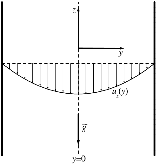
Figure 1: Sketch of the planar Poiseuille flow induced by a gravitational force.

As done in laboratory experiments (and in computer simulations), we will assume that energy is externally injected into the system to compensate for the collisional cooling, so that a steady state is achieved even if the gravity field is formally switched off. In real experiments, BK01 ; LCDKG99 ; FWEFCGB99 this is usually achieved by means of boundary vibrations of small amplitude $A\sim\sigma$ and high frequency $\omega/2\pi\sim 10$–$100~{}\text{Hz}$, so that the maximum accelaration $\Gamma=A\omega^{2}$ is usually several times larger than the acceleration due to gravity on Earth. However, this type of realistic heating through the boundaries is difficult to deal with at a theoretical level due to unavoidable boundary effects. These difficulties are overcome by assuming a bulk heating mechanism acting on all the particles simultaneously. The most commonly used type of bulk driving for inelastic particles consists of a stochastic force in the form of Gaussian white noise WM96 ; vNE98 ; SBCM98 ; vNETP99 ; BSSS99 ; MS00 ; BNK00 ; CCG00 . More precisely, each particle $i$ is subject to the action of a stochastic force ${\bf F}_{i}(t)$ that has the properties

$$\langle{\bf F}_{i}(t)\rangle={\bf 0},\quad\langle{\bf F}_{i}(t){\bf F}_{j}(t^{\prime})\rangle={\sf I}m^{2}\xi^{2}\delta_{ij}\delta(t-t^{\prime}),$$ (16)

where ${\sf I}$ is the $3\times 3$ unit matrix and $\xi^{2}$ represents the strenght of the correlation. According to this white noise driving, during a small time step $\delta t$ each particle $i$ receives an independent “kick” such that its velocity is incremented by a random value $\delta\mathbf{v}_{i}$ with the statistical propertiesMS00

$$\langle\delta{\bf v}_{i}\rangle={\bf 0},\quad\langle\delta{\bf v}_{i}\delta{\bf v}_{j}\rangle={\sf I}\xi^{2}\delta t\delta_{ij}.$$ (17)

Therefore, $|\delta\mathbf{v}|\sim\xi\sqrt{\delta t}$. The associated operator $\mathcal{F}$ appearing in the Boltzmann equation (1) isvNE98

$$\mathcal{F}=-\frac{\xi^{2}}{2}\left(\frac{\partial}{\partial{\bf v}}\right)^{2}.$$ (18)

Thus $\xi^{2}/2$ plays the role of a diffusion coefficient in velocity space. The operator (18) verifies the properties (12), while insertion into Eq. (11) shows that the heating rate is

$$\gamma=\frac{m\xi^{2}}{T}.$$ (19)

It still remains to define the spatial dependence of $\gamma$. By simplicity, we assume that the white noise driving compensates locally for the collisional energy loss. This means that $\gamma=\zeta$ or, equivalently, $\xi=\sqrt{\zeta T/m}$ at any point. This choice can be justified by the following argument. Since, as seen above, $|\delta\mathbf{v}|\sim\xi\sqrt{\delta t}$, the choice $\gamma=\zeta$ implies that

$$\frac{|\delta\mathbf{v}|}{v_{\text{th}}}\sim\sqrt{\nu\delta t(1-\alpha^{2})},$$ (20)

where use has been made of Eq. (14) and of $v_{\text{th}}\sim\sqrt{T/m}$. Equation (20) means that the relative random increment of velocity at a given point scales as the square root of the average collision number at that point. When heating the gas through the boundaries, the energy input is propagated to the whole system by means of collisions. Since the white noise driving intends to mimic that effect, it is quite natural that the relative magnitude of the kicks is larger in those regions where the collisions are more frequent.

By considering the above white noise excitation mechanism, a steady state can be expected in which the physical quantities depend on the coordinate $y$ only and the flow velocity is parallel to the $z$ axis, ${\bf u}=u_{z}(y)\widehat{\bf z}$. In that case, the Boltzmann equation (1) becomes

$$\left(-\frac{\zeta T}{2m}\frac{\partial^{2}}{\partial{\bf v}^{2}}-g\frac{\partial}{\partial v_{z}}+v_{y}\frac{\partial}{\partial y}\right)f=J[f,f].$$ (21)

Similarly, the balance equations for momentum and energy, Eqs. (6) and (7), reduce to

$$\frac{\partial P_{yy}}{\partial y}=0,$$ (22)

$$\frac{\partial P_{yz}}{\partial y}=-\rho g,$$ (23)

$$P_{yz}\frac{\partial u_{z}}{\partial y}+\frac{\partial q_{y}}{\partial y}=0,$$ (24)

where $\rho=mn$ is the mass density. Note that the inelasticity does not appear explicitly in the balance equations (22)–(24).

II.3 Navier–Stokes description

In the Newtonian description the fluxes are related to the hydrodynamic gradients by the Navier–Stokes (NS) constitutive equations.BDKS98 ; GD99 ; GM01 In the geometry of the Poiseuille problem they read

$$P_{xx}=P_{yy}=P_{zz}=p,$$ (25)

$$P_{yz}=-\eta\frac{\partial u_{z}}{\partial y},$$ (26)

$$q_{y}=-\kappa\frac{\partial T}{\partial y}-\mu\frac{\partial n}{\partial y},$$ (27)

$$q_{z}=0,$$ (28)

where $p=nT=\frac{1}{3}\mbox{Tr}\,{\sf P}$ is the hydrostatic pressure, $\eta$ is the the shear viscosity, $\kappa$ is the thermal conductivity, and $\mu$ is a transport coefficient with no analog for elastic fluids. These transport coefficients can be explicitly derived from the Boltzmann equation (1) by application of the Chapman–Enskog method in the first Sonine approximation. In the case of the white noise heating (18) with $\xi=\sqrt{\zeta T/m}$ their expressions areGM01

$$\eta=\frac{p}{\nu_{\eta}},\quad\kappa=\frac{5p}{2m\nu_{\kappa}}\left(1+2k\right),\quad\mu=\frac{5T^{2}}{2m\nu_{\kappa}}{k},$$ (29)

where

$$\nu_{\eta}=\frac{\nu}{4}(1+\alpha)\left(3-\alpha\right)\left(1-\frac{1}{32}k\right),$$ (30)

$$\nu_{\kappa}=\frac{\nu}{3}(1+\alpha)\left(\frac{49-33\alpha}{16}+\frac{19-3\alpha}{512}k\right).$$ (31)

In the above equations, $\nu$ is the effective collision frequency defined by Eq. (15) and $k$ is the kurtosis of the homogeneous heated state. Its expression is well approximated byvNE98

$$k=\frac{16(1-\alpha)(1-2\alpha^{2})}{241-177\alpha+30\alpha^{2}(1-\alpha)}.$$ (32)

The kurtosis $k$ is rather small for all $\alpha$. In particular, $|k|<0.013$ for $0.6\leq\alpha\leq 1$. Therefore, one can neglect $k$ in (29)–(31) to get

$$\eta\simeq\frac{p}{\nu}\frac{4}{(1+\alpha)\left(3-\alpha\right)},\quad\kappa\simeq\frac{5p}{2m\nu}\frac{48}{(1+\alpha)\left(49-33\alpha\right)},\quad\mu\simeq 0.$$ (33)

In the interval $0.6\leq\alpha\leq 1$, the expressions (33) for $\eta$ and $\kappa$ deviate from those of (29) less than 0.04% and 3%, respectively. Besides, the ratio $n\mu/T\kappa$ is smaller than 0.013, so that $\mu$ can be neglected. Note that the negligible role played by $\mu$ does not hold in the homogeneous cooling state.BDKS98 ; GD99 It is worth pointing out that, while the shear viscosity monotonically increases with inelasticity, the thermal conductivity starts decreasing with increasing inelasticity, reaches a minimum value around $\alpha=0.4$, and then slightly increases for $\alpha\gtrsim 0.4$. This non-monotonic behavior of $\kappa$ in the heated state contrasts with the one found in the free cooling case.BDKS98 ; GM01 ; S03

Combining Eqs. (22)–(27), we get

$$\frac{\partial p}{\partial y}=0,$$ (34)

$$\frac{\partial}{\partial y}\eta\frac{\partial u_{z}}{\partial y}=\rho g,$$ (35)

$$\frac{\partial}{\partial y}\kappa^{\prime}\frac{\partial T}{\partial y}=-\eta\left(\frac{\partial u_{z}}{\partial y}\right)^{2},$$ (36)

where $\kappa^{\prime}=\kappa-n\mu/T\simeq\kappa$. Equation (35) gives a parabolic-like velocity profile, that is characteristic of the Poiseuille flow. The temperature profile has, according to Eq. (36), a quartic-like shape. Strictly speaking, these NS profiles are more complicated than just polynomials due to the temperature dependence of the transport coefficients. Since the hydrodynamic profiles must be symmetric with respect to the middle plane $y=0$, their odd derivatives must vanish at $y=0$. Thus, from Eqs. (35) and (36) we have

$$\left.\frac{\partial^{2}u_{z}}{\partial y^{2}}\right|_{y=0}=\frac{\rho_{0}g}{\eta_{0}},\quad\left.\frac{\partial^{2}T}{\partial y^{2}}\right|_{y=0}=0,\quad\left.\frac{\partial^{4}T}{\partial y^{4}}\right|_{y=0}=-2\frac{\rho_{0}^{2}g^{2}}{\eta_{0}\kappa_{0}^{\prime}},$$ (37)

where the subscript $0$ denotes quantities evaluated at $y=0$. According to Eq. (37), the NS equations predict that the temperature has a maximum at the middle layer $y=0$. As we will see in Sec. III, the kinetic theory description shows that the temperature actually exhibits a local minimum at $y=0$, since $\left.\partial^{2}T/\partial y^{2}\right|_{y=0}$ is a positive quantity (of order $g^{2}$).

The closed set of nonlinear equations (34)–(36) cannot be solved analytically for arbitrary $g$ due to the spatial dependence of the transport coefficients. On the other hand, if the acceleration of gravity is sufficiently small at the microscopic scale, we can expand in powers of $g$ and keep the first few terms only. To second order, the NS hydrodynamic profiles near the layer $y=0$ are

$$u_{z}(y)=u_{0}+\frac{\rho_{0}g}{2\eta_{0}}{y}^{2}+{\cal O}(g^{3}),$$ (38)

$$T(y)=T_{0}-\frac{\rho_{0}^{2}g^{2}}{12\eta_{0}\kappa_{0}^{\prime}}{y}^{4}+{\cal O}(g^{4}).$$ (39)

The space variable $y$ can be eliminated between Eqs. (38) and (39) to obtain the following nonequilibrium “equation of state”:

$$T=T_{0}-\frac{\eta_{0}}{3\kappa_{0}^{\prime}}(u_{0}-u_{z})^{2}+{\cal O}(g^{4}).$$ (40)

The NS profiles for the fluxes are

$$P_{yz}(y)=-\rho_{0}g{y}+{\cal O}(g^{3}),$$ (41)

$$q_{y}(y)=\frac{\rho_{0}^{2}g^{2}}{3\eta_{0}}{y}^{3}+{\cal O}(g^{4}).$$ (42)

III Kinetic theory description

III.1 A kinetic model

In this Section we will see that most of the NS predictions discussed in the preceding Subsection do not hold true, even to first order in $g$, when the problem is attacked from a more detailed kinetic point of view. In principle, the task consists of solving the Boltzmann equation (21) through order $g^{2}$ in a region near the central layer $y=0$.

Given the mathematical complexity of the Boltzmann collision operator (2), especially in the case of inelastic collisions, we simplify the analysis by replacing $J[f,f]$ by a BGK-like kinetic model:BDS99 ; SA04

$$J[f,f]\to-\beta(\alpha)\nu(f-f_{\ell})+\frac{\zeta_{\ell}}{2}\frac{\partial}{\partial{\bf v}}\cdot\left[\left({\bf v-u}\right)f\right],$$ (43)

where $\nu$ is the collision frequency (15), $f_{\ell}$ is the local Maxwellian distribution (13), and $\zeta_{\ell}$ is the associated cooling rate (14). In addition, $\beta(\alpha)$ is a dimensionless function of the coefficient of restitution that can be freely chosen to optimize agreement with the Boltzmann description. Equation (43) differs from the original formulation of the model kinetic equationBDS99 in that the exact (local) homogeneous cooling state of the Boltzmann equation is replaced by $f_{\ell}$ and the exact cooling rate (10) is approximated by $\zeta_{\ell}$. Confirmation of the quantitative agreement between the kinetic model and the Boltzmann equation has been found for the simple shear flowBRM97 ; MGSB99 and the nonlinear Couette flow.TTMGSD01

The first term on the right-hand side of (43) describes collisional relaxation towards the local Maxwellian with a collision rate $\beta\nu$, while the second term describes the dominant collisional cooling effects. The necessity for this term to accurately represent the spectrum of the Boltzmann collision operator is discussed in Ref. BDS99, . However, it can be viewed more simply as an effective “drag” force that produces the same energy loss rate as that produced by the inelastic collisions. The NS transport coefficients derived from the model (43) in the case of white noise heating areS03

$$\eta=\frac{p}{\beta\nu+\zeta_{\ell}},\quad\kappa=\frac{5p}{2m\left(\beta\nu+\frac{3}{2}\zeta_{\ell}\right)},\quad\mu=0.$$ (44)

A simple choice for the parameter $\beta$ is $\beta=\frac{1}{2}(1+\alpha)$.SA04 On the other hand, comparison with the (approximate) Boltzmann results (33) shows that the shear viscosity is reproduced if $\beta$ takes the value

$$\beta=(1+\alpha)\frac{2+\alpha}{6},$$ (45)

while the thermal conductivity is reproduced if

$$\beta=(1+\alpha)\frac{19-3\alpha}{48}.$$ (46)

The discrepancy between Eqs. (45) and (46) persists in the elastic limit ($\alpha=1$) and is a well-known limitation of the BGK model. As will be seen in Sec. IV, one can partially circumvent this problem by expressing the final results in terms of $\eta$ and $\kappa$.

Inserting the model (43) into Eq. (21), we get the kinetic equation

$$\left(-g\frac{\partial}{\partial v_{z}}+v_{y}\frac{\partial}{\partial y}\right)f=-\beta\nu(f-f_{\ell})+\frac{\zeta_{\ell}}{2}\frac{\partial}{\partial{\bf v}}\cdot\left({\bf V}+\frac{T}{m}\frac{\partial}{\partial{\bf v}}\right)f,$$ (47)

where, for consistency, we have made the approximation $\zeta\to\zeta_{\ell}$ in Eq. (21). In order to focus on the deviations from the local equilibrium distribution, let us write

$$f=f_{\ell}(1+\Phi).$$ (48)

Then, Eq. (47) becomes

$$(1+\Phi)\left[V_{y}\widetilde{\partial}_{y}\log f_{\ell}-\left(g+V_{y}\frac{\partial u_{z}}{\partial y}\right)\frac{\partial}{\partial V_{z}}\log f_{\ell}\right]=$$

$$\left(g+V_{y}\frac{\partial u_{z}}{\partial y}\right)\frac{\partial}{\partial V_{z}}\Phi-V_{y}\widetilde{\partial}_{y}\Phi-(\nu^{\prime}-\zeta_{\ell})\Phi+\frac{\zeta_{\ell}}{2}\left(\frac{T}{m}\frac{\partial}{\partial{\bf V}}-{\bf V}\right)\cdot\frac{\partial}{\partial{\bf V}}\Phi,$$

(49)

where the operator $\widetilde{\partial}_{y}\equiv\partial/\partial y+(\partial u_{z}/\partial y)\partial/\partial V_{z}$ derives with respect to $y$ at constant ${\bf V}$ (i.e., not at constant ${\bf v}$). Moreover, in Eq. (49) we have introduced the modified collision frequency $\nu^{\prime}\equiv\beta\nu+\zeta_{\ell}$. As Eq. (44) shows, $\nu^{\prime}$ is the effective collision frequency associated with the shear viscosity of the heated granular gas in the kinetic model.

Since we are interested in the solution of Eq. (49) in the bulk, it is convenient to take the state at the mid point $y=0$ as a reference state and define the following dimensionless quantities:

$${\bf V}^{*}={\bf V}/v_{0},\quad y^{*}=y\nu_{0}^{\prime}/v_{0},\quad f_{\ell}^{*}=f_{\ell}v_{0}^{3}/n_{0},$$ (50)

$$p^{*}=p/p_{0},\quad{\bf u}^{*}={\bf u}/v_{0},\quad T^{*}=T/T_{0},\quad g^{*}=g/\nu_{0}^{\prime}v_{0}$$ (51)

$${\nu^{\prime}}^{*}=\nu^{\prime}/\nu_{0}^{\prime},\quad\mathsf{P}^{*}={\sf P}/p_{0},\quad{\bf q}^{*}={\bf q}/p_{0}v_{0},$$ (52)

where, as in Eqs. (37)–(42), the subscript 0 denotes quantities at $y=0$. In particular, $v_{0}=(2T_{0}/m)^{1/2}$ is the thermal velocity $v_{\text{th}}$ at $y=0$. The reduced quantity $y^{*}$ measures distance in units of a nominal mean free path, while $g^{*}$ measures the strength of the gravity field on a particle moving with the thermal velocity along a distance of the order of the mean free path. The choice of $1/\nu_{0}^{\prime}$ (which depends on $\alpha$) instead of $1/\nu_{0}$ (which is independent of $\alpha$) as the time unit is suggested by a larger simplicity in the calculations stemming from the kinetic model. In any case, in Section IV we will summarize the results in real units, so the final expressions are independent of the specific choice of reduced quantities.

In the above units, the kinetic equation (49) becomes

$$(1+\Phi)\left[V_{y}^{*}\widetilde{\partial}_{y^{*}}\log f_{\ell}^{*}+\frac{2V_{z}^{*}}{T^{*}}\left(g^{*}+V_{y}^{*}\frac{\partial u_{z}^{*}}{\partial y^{*}}\right)\right]=\left(g^{*}+V_{y}^{*}\frac{\partial u_{z}^{*}}{\partial y^{*}}\right)\frac{\partial}{\partial V_{z}^{*}}\Phi$$

$$-V_{y}^{*}\widetilde{\partial}_{y^{*}}\Phi-{\nu^{\prime}}^{*}\left(1-\zeta_{0}^{*}\right)\Phi+\zeta_{0}^{*}\frac{{\nu^{\prime}}^{*}}{2}\left(\frac{T^{*}}{2}\frac{\partial}{\partial{\bf V}^{*}}-{\bf V}^{*}\right)\cdot\frac{\partial}{\partial{\bf V}^{*}}\Phi,$$

(53)

where

$$\widetilde{\partial}_{y^{*}}\log f_{\ell}^{*}=\frac{\partial\log p^{*}}{\partial y^{*}}+\left(\frac{V^{2}}{T}-\frac{5}{2}\right)\frac{\partial\log T^{*}}{\partial y^{*}}.$$ (54)

On the right-hand side of Eq. (53) we have taken into account that $\zeta_{\ell}=\zeta_{0}^{*}\nu^{\prime}$, where [cf. Eq. (14)]

$$\zeta_{0}^{*}=\frac{\frac{5}{12}(1-\alpha^{2})}{\beta(\alpha)+\frac{5}{12}(1-\alpha^{2})}$$ (55)

is a pure number that only depends on the coefficient of restitution. It gives the cooling rate at any given point in units of the modified collision frequency $\nu^{\prime}$ at that same point.

Our purpose is to solve Eq. (53) to second order in $g^{*}$ and get the associated hydrodynamic profiles.

III.2 Perturbation expansion

In this Subsection, all the quantities will be understood to be expressed in reduced units and the asterisks will be dropped. The expansion of $\Phi$ in powers of $g$ is

$$\Phi=\Phi^{(1)}g+\Phi^{(2)}g^{2}+{\cal O}(g^{3}),$$ (56)

where we have taken into account that the solution of Eq. (47) in the absence of gravity is $f=f_{\ell}$ with uniform $n$, $\mathbf{u}$, and $T$. The expansions for the hydrodynamic fields have the forms

$$p=1+p^{(2)}g^{2}+{\cal O}(g^{4}),$$ (57)

$$u_{z}=u^{(1)}g+{\cal O}(g^{3}),$$ (58)

$$T=1+T^{(2)}g^{2}+{\cal O}(g^{4}).$$ (59)

Here we have taken into account that, because of the symmetry of the problem, $p$ and $T$ are even functions of $g$, while $u_{z}$ is an odd function. Also, without loss of generality, we have taken $u_{0}=0$, i.e., we are performing a Galilean change to a reference frame moving with the fluid at $y=0$. Since $\nu^{\prime}=pT^{-1/2}$, we have

$$\nu^{\prime}=1+\left(p^{(2)}-\frac{1}{2}T^{(2)}\right)g^{2}+{\cal O}(g^{4}).$$ (60)

Nevertheless, only $\nu^{\prime}=1$ is needed in the evaluation of $\Phi^{(1)}$ and $\Phi^{(2)}$.

In order to solve Eq. (53) at each order, we will need to use the consistency conditions

$$\int d{\bf V}\,f_{\ell}\Phi=0,$$ (61)

$$\int d{\bf V}\,V_{y}f_{\ell}\Phi=0,$$ (62)

$$\int d{\bf V}\,V_{z}f_{\ell}\Phi=0,$$ (63)

$$\int d{\bf V}\,V^{2}f_{\ell}\Phi=0.$$ (64)

III.2.1 First order

To first order in $g$, Eq. (53) yields

$$\left(1-{\cal A}\right)\Phi^{(1)}=-\frac{2}{1-\zeta_{0}^{*}}V_{z}\left(1+V_{y}\frac{\partial u^{(1)}}{\partial y}\right)\equiv\phi^{(1)},$$ (65)

where ${\cal A}$ is the operator

$${\cal A}=\frac{\zeta_{0}^{*}}{2(1-\zeta_{0}^{*})}\left(\frac{1}{2}\frac{\partial}{\partial{\bf V}}-{\bf V}\right)\cdot\frac{\partial}{\partial{\bf V}}-\frac{1}{1-\zeta_{0}^{*}}V_{y}\widetilde{\partial}_{y}.$$ (66)

The function $\phi^{(1)}$ has a known velocity dependence. Its space dependence occurs through $u^{(1)}$, which remains unknown so far. In order to solve Eq. (65), we will follow a heuristic procedure. First, we guess that the first-order velocity profile is parabolic:

$$u^{(1)}(y)=u^{(1)}_{2}y^{2}.$$ (67)

Next, we note that the formal solution to Eq. (65) is $\Phi^{(1)}=\sum_{k=0}^{\infty}{\cal A}^{k}\phi^{(1)}$ and that the functional structure of ${\cal A}^{k}\phi^{(1)}$ remains the same for any $k$. Consequently, the solution to Eq. (65) must have such a structure, namely

$$\Phi^{(1)}(y,\mathbf{V})=V_{z}(a_{0}+a_{1}V_{y}^{2}+a_{2}V_{y}y).$$ (68)

Equations (67) and (68) have the same structure as the solution of the BGK equation in the elastic case.TS94 ; TS01 Insertion of Eq. (68) into Eq. (65) allows one to identify the coefficients $a_{0},a_{1},a_{2}$. The result is

$$a_{0}=4\frac{2\zeta_{0}^{*}u^{(1)}_{2}-\zeta_{0}^{*}-2}{4-{\zeta_{0}^{*}}^{2}},\quad a_{1}=\frac{8u^{(1)}_{2}}{2+\zeta_{0}^{*}},\quad a_{2}=-4u^{(1)}_{2}.$$ (69)

The consistency conditions (61), (62), and (64) are verified by symmetry. The coefficient $u^{(1)}_{2}$ is determined by the condition (63) with the result

$$u^{(1)}_{2}=1.$$ (70)

Once we know $\Phi^{(1)}$ explicitly, we can get the non-zero components of the fluxes to first order. They are

$$P_{yz}^{(1)}(y)=2\int d{\bf V}\,V_{y}V_{z}f_{0}\Phi^{(1)}=-2y$$ (71)

$$q_{z}^{(1)}(y)=\int d{\bf V}\,V^{2}V_{z}f_{0}\Phi^{(1)}=\frac{2}{2+\zeta_{0}^{*}},$$ (72)

where $f_{0}=\pi^{-3/2}e^{-V^{2}}$ is $f_{\ell}$ at $y=0$.

III.2.2 Second order

We proceed in a similar way as before. The equation for $\Phi^{(2)}$ is

$$\left(1-{\cal A}\right)\Phi^{(2)} = \frac{1}{1-\zeta_{0}^{*}}\left(1+V_{y}\frac{\partial u^{(1)}}{\partial y}\right)\left(\frac{\partial}{\partial V_{z}}-2V_{z}\right)\Phi^{(1)}$$ (73)

$$-\frac{V_{y}}{1-\zeta_{0}^{*}}\left[\frac{\partial p^{(2)}}{\partial y}+\left({V^{2}}-\frac{5}{2}\right)\frac{\partial T^{(2)}}{\partial y}\right]\equiv\phi^{(2)}.$$

Now, we guess the profiles

$$p^{(2)}(y)=p^{(2)}_{2}y^{2},$$ (74)

$$T^{(2)}(y)=T^{(2)}_{2}y^{2}+T^{(2)}_{4}y^{4}.$$ (75)

The structure of ${\cal A}^{k}\phi^{(2)}$ suggests the trial function

$$\Phi^{(2)}(y,\mathbf{V}) = b_{0}+b_{1}V_{y}^{2}+b_{2}V_{y}y+b_{3}y^{2}+b_{4}V_{y}^{4}+b_{5}V_{y}^{3}y+b_{6}V_{y}^{2}y^{2}$$ (76)

$$+b_{7}V_{y}y^{3}+V_{z}^{2}\left(c_{0}+c_{1}V_{y}^{2}+c_{2}V_{y}y+c_{3}y^{2}+c_{4}V_{y}^{4}\right.$$

$$\left.+c_{5}V_{y}^{3}y+c_{6}V_{y}^{2}y^{2}\right)+V^{2}\left(d_{0}+d_{1}V_{y}^{2}+d_{2}V_{y}y+d_{3}y^{2}\right.$$

$$\left.+d_{4}V_{y}^{4}+d_{5}V_{y}^{3}y+d_{6}V_{y}^{2}y^{2}+d_{7}V_{y}y^{3}\right).$$

Insertion into Eq. (73) allows one to get the coefficients $b_{i}$, $c_{i}$, and $d_{i}$ in terms of $p_{2}^{(2)}$, $T_{2}^{(2)}$, and $T_{4}^{(2)}$. Condition (62) is identically satisfied regardless of the values of $p_{2}^{(2)}$, $T_{2}^{(2)}$, and $T_{4}^{(2)}$, while Eq. (63) is verified by symmetry. On the other hand, conditions (61) and (64) yield

$$p_{2}^{(2)}=\frac{24}{5},\quad T_{2}^{(2)}=\frac{4}{25}\frac{38+43\zeta_{0}^{*}+17{\zeta_{0}^{*}}^{2}}{(1+\zeta_{0}^{*})(2+\zeta_{0}^{*})},\quad T_{4}^{(2)}=-\frac{2}{15}(2+\zeta_{0}^{*}).$$ (77)

The expressions of the coefficients $b_{i}$, $c_{i}$, and $d_{i}$ as functions of $\alpha$ are given in Appendix A. From $\Phi^{(2)}$ we can calculate the second order contributions to the fluxes:

$$P_{yy}^{(2)}=p^{(2)}+2\int d{\bf V}\,V_{y}^{2}f_{0}\Phi^{(2)}=-\frac{24}{25}\frac{102+87\zeta_{0}^{*}+13{\zeta_{0}^{*}}^{2}}{(1+\zeta_{0}^{*})(2+\zeta_{0}^{*})^{2}},$$ (78)

$$P_{zz}^{(2)}(y)=p^{(2)}+2\int d{\bf V}\,V_{z}^{2}f_{0}\Phi^{(2)}=\frac{32}{25}\frac{82+67\zeta_{0}^{*}+8{\zeta_{0}^{*}}^{2}}{(1+\zeta_{0}^{*})(2+\zeta_{0}^{*})^{2}}+\frac{56}{5}y^{2},$$ (79)

$$q_{y}^{(2)}(y)=\int d{\bf V}\,V^{2}V_{y}^{2}f_{0}\Phi^{(2)}=\frac{4}{3}y^{3}.$$ (80)

IV Summary and discussion

IV.1 Hydrodynamic profiles

Let us summarize here the main results obtained from the kinetic model through second order in the gravity field. The hydrodynamic profiles are given by Eqs. (57)–(59), (67), (70), (74), (75), and (77). Expressed in real units, they are

$$p(y)=p_{0}\left[1+\frac{6}{5}\left(\frac{mg}{T_{0}}\right)^{2}y^{2}\right]+{\cal O}(g^{4}),$$ (81)

$$u_{z}(y)=u_{0}+\frac{\rho_{0}g}{2\eta_{0}}{y}^{2}+{\cal O}(g^{3}),$$ (82)

$$T(y)=T_{0}\left[1-\frac{\rho_{0}^{2}g^{2}}{12\eta_{0}\kappa_{0}T_{0}}{y}^{4}+\frac{1}{25}\frac{38+43\zeta_{0}^{*}+17{\zeta_{0}^{*}}^{2}}{(1+\zeta_{0}^{*})(2+\zeta_{0}^{*})}\left(\frac{mg}{T_{0}}\right)^{2}y^{2}\right]+{\cal O}(g^{4}).$$ (83)

In Eqs. (82) and (83), $\eta_{0}$ and $\kappa_{0}=\kappa^{\prime}_{0}$ are the NS transport coefficients (evaluated at the mid point $y=0$) of the granular gas heated by the stochastic force. In the kinetic model, those transport coefficients are given by Eq. (44). Note that the elimination of the collision frequencies $\nu$ or $\nu^{\prime}=\beta\nu+\zeta_{\ell}$ in favor of the transport coefficients $\eta$ and $\kappa$ allows us to circumvent the limitation inherent to BGK-like models of not giving the correct Prandtl number. In that way, Eqs. (81)–(83) can be expected to be close to the Boltzmann results, as happens in the elastic case.TSS98 ; STS03 Therefore, in what follows we will use for $\eta$ and $\kappa$ the Boltzmann expressions (33). In Eq. (83) the parameter $\zeta_{0}^{*}$ is given by Eq. (55), where $\beta(\alpha)$ can be freely chosen. Here we will take the choice (45), which makes the NS shear viscosity of the kinetic model agree with that of the Boltzmann equation.

Comparison of Eqs. (81)–(83) with the NS predictions, Eqs. (34), (38), and (39) shows that the latter provide an incomplete description to second order in $g$. According to the kinetic theory description, the pressure increases parabolically from the mid layer rather than being uniform and the temperature has an extra positive quadratic term that is responsible for the fact that the temperature has a local minimum at $y=0$ rather than a maximum. This minimum is surrounded by two symmetric maxima located at a distance ($y_{\text{max}}$) from $y=0$ of the order of a few mean free paths. Analogously, the NS equation of state (40) is corrected by an extra term,

$$T=T_{0}-\frac{\eta_{0}}{3\kappa_{0}}(u_{0}-u_{z})^{2}+\frac{1}{30}\frac{38+43\zeta_{0}^{*}+17{\zeta_{0}^{*}}^{2}}{(1+\zeta_{0}^{*})(2+\zeta_{0}^{*})}(p-p_{0})+{\cal O}(g^{4}).$$ (84)

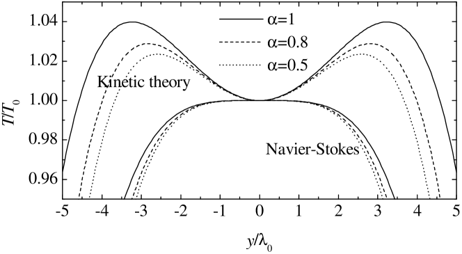
Figure 2: Temperature profiles for $g\lambda_{0}/v_{0}^{2}=0.05$ and $\alpha=0.5$ (dotted lines), $\alpha=0.8$ (dashed lines), and $\alpha=1$ (solid lines), as predicted by the Navier–Stokes and kinetic theory descriptions.

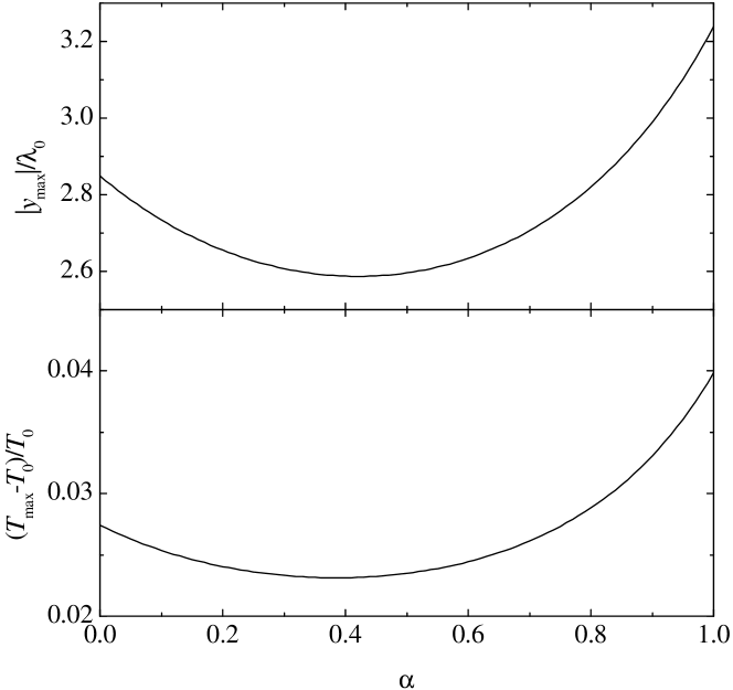
Figure 3: Plot of $|y_{\text{max}}|/\lambda_{0}$ and $(T_{\text{max}}-T_{0})/T_{0}$ versus $\alpha$. In the latter case we have taken $g\lambda_{0}/v_{0}^{2}=0.05$.

In order to analyze in detail the temperature profile (83), let us measure the coordinate $y$ in units of the mean free path $\lambda_{0}=(\pi\sqrt{2}n_{0}\sigma^{2})^{-1}=(8/5\sqrt{\pi})v_{0}/\nu_{0}$, where $v_{0}=\sqrt{2T_{0}/m}$ is the thermal velocity and $\nu_{0}$ is the collision frequency (15), both at $y=0$. Thus, Eq. (84) becomes

$$\frac{T(y)}{T_{0}}=1-A_{4}(\alpha)\left(\frac{g\lambda_{0}}{v_{0}^{2}}\right)^{2}\left(\frac{y}{\lambda_{0}}\right)^{4}+A_{2}(\alpha)\left(\frac{g\lambda_{0}}{v_{0}^{2}}\right)^{2}\left(\frac{y}{\lambda_{0}}\right)^{2}+\mathcal{O}(g^{4}),$$ (85)

where

$$A_{4}(\alpha)=\frac{4}{1125\pi}(1+\alpha)^{2}(3-\alpha)(49-33\alpha),\quad A_{2}=\frac{4}{25}\frac{2719-2741\alpha+706\alpha^{2}}{(7-4\alpha)(23-11\alpha)}.$$ (86)

The coefficient $A_{2}(\alpha)$ monotonically decreases with increasing inelasticity, while $A_{4}(\alpha)$ has a maximum at $\alpha\simeq 0.46$, essentially due to the non-monotonic behavior of the thermal conductivity.

The location $y_{\text{max}}$ of the two symmetric maxima is

$$y_{\text{max}}=\pm\lambda_{0}\sqrt{\frac{A_{2}(\alpha)}{2A_{4}(\alpha)}}.$$ (87)

Note that, in the regime $g\lambda_{0}/v_{0}^{2}\ll 1$, $y_{\text{max}}$ is independent of the precise value of $g$. The relative value of the maximum temperature is

$$\frac{T_{\text{max}}-T_{0}}{T_{0}}=\frac{A_{2}^{2}(\alpha)}{4A_{4}(\alpha)}\left(\frac{g\lambda_{0}}{v_{0}^{2}}\right)^{2}+\mathcal{O}(g^{4}).$$ (88)

Of course, if we formally make $A_{2}(\alpha)=0$ in Eq. (85), the NS temperature profile (39) is recovered.

As an illustration of the corrections over the NS description provided by the kinetic model, let us consider a value $g\lambda_{0}/v_{0}^{2}=0.05$. In the case of terrestrial gravity, the above value corresponds, for instance, to $\lambda_{0}\sim 5~{}\text{mm}$ and $v_{0}\sim 1~{}\text{m/s}$. Although terms of order higher than $g^{2}$ in (85) might not be negligible for this particular value of $g\lambda_{0}/v_{0}^{2}$, the qualitative features are expected to remain correct. Figure 2 shows the temperature profiles for a granular gas with $\alpha=0.5$ and $\alpha=0.8$, as well as for a gas of elastic particles ($\alpha=1$), as predicted by the NS and kinetic theory descriptions. We observe that strong deviations from the NS profiles are apparent, both for elastic and inelastic systems. Focusing now on the profiles predicted by the kinetic model, we se that, as the inelasticity increases, the locations of the two maxima shift towards the center of the slab and the value of the maximum temperature decreases. This behavior, however, is reversed if $\alpha\lesssim 0.4$. The $\alpha$-dependence of $|y_{\text{max}}|/\lambda_{0}$ and $(T_{\text{max}}-T_{0})/T_{0}$ is displayed in Fig. 3. The non-monotonic behaviors of $y_{\text{max}}$ and $T_{\text{max}}$ are consequences of that of $A_{4}(\alpha)$.

IV.2 Fluxes

The profiles for the elements of the pressure tensor and the components of the heat flux through second order are given by Eqs. (71), (72), and (78)–(80). Expressed in real units, they are

$$P_{yz}(y)=-\rho_{0}g{y}+{\cal O}(g^{3}),$$ (89)

$$P_{yy}=p_{0}\left[1-\frac{12}{25}\frac{102+87\zeta_{0}^{*}+13{\zeta_{0}^{*}}^{2}}{(1+\zeta_{0}^{*})(2+\zeta_{0}^{*})^{2}}\frac{\rho_{0}\eta_{0}^{2}g^{2}}{p_{0}^{3}}\right]+{\cal O}(g^{4}),$$ (90)

$$P_{zz}(y)=p_{0}\left[1+\frac{16}{25}\frac{82+67\zeta_{0}^{*}+8{\zeta_{0}^{*}}^{2}}{(1+\zeta_{0}^{*})(2+\zeta_{0}^{*})^{2}}\frac{\rho_{0}\eta_{0}^{2}g^{2}}{p_{0}^{3}}+\frac{14}{5}\left(\frac{mg}{T_{0}}\right)^{2}y^{2}\right]+{\cal O}(g^{4}),$$ (91)

$$q_{y}(y)=\frac{\rho_{0}^{2}g^{2}}{3\eta_{0}}{y}^{3}+{\cal O}(g^{4}),$$ (92)

$$q_{z}=\frac{2}{5}m\kappa_{0}g+{\cal O}(g^{3}).$$ (93)

The $xx$-element of the pressure tensor is $P_{xx}=3p-P_{yy}-P_{zz}$. Note that $P_{yy}$ is uniform, in agreement with the exact balance equation (22). Likewise, it is easy to check that Eqs. (82), (89), and (92) are consistent with the energy balance equation (24). Moreover, since the density profile is known through second order [cf. Eqs. (81) and (83)], Eq. (23) can be used to get $P_{yz}$ through third order.

The shear stress $P_{yz}$ agrees to second order in $g$ with Newton’s viscosity law (26). However, the component $q_{y}$ of the heat flux parallel to the thermal gradient does not obey Fourier’s law (27) (note that $\mu\approx 0$ in the heated state). In fact, from Eqs. (83) and (92) one can write an

$$q_{y}=-\kappa\frac{\partial}{\partial y}\left(T+\frac{y_{\text{max}}^{2}}{6}\nabla^{2}T\right)+\mathcal{O}(g^{4}),$$ (94)

which shows that one needs to incorporate super-Burnett contributions to account for the relationship between the heat flux and the thermal gradients. The extra term on the right-hand side of Eq. (94) is responsible for the counter-intuitive fact of $q_{y}$ having the same sign as $\partial T/\partial y$ in the region $0\leq|y|<|y_{\text{max}}|$, i.e., the temperature increases as one moves away from the mid layer $y=0$ and yet the heat flows outward from the colder to the hotter layers. A steady state is still possible because the energy deficit is compensated for by the viscous heating. An additional departure from Fourier’s law is related to the existence of a component $q_{z}$ of the heat flux normal to the thermal gradient, an effect that is already of first order in $g$ and is related to a Burnett contribution associated with $\nabla^{2}u_{z}$.TSS98

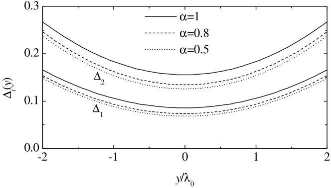
Figure 4: Profiles of the normal stress differences $\Delta_{1}=(P_{zz}-P_{xx})/{p}$ and $\Delta_{2}=(P_{zz}-P_{yy})/{p}$ for $g\lambda_{0}/v_{0}^{2}=0.05$ and $\alpha=0.5$ (dotted lines), $\alpha=0.8$ (dashed lines), and $\alpha=1$ (solid lines). Note that $\Delta_{1}=\Delta_{2}=0$ in the NS description.

Equations (81), (90), and (91) show that normal stress differences appear to order $g^{2}$. It is easy to check that $P_{yy}<P_{xx}<p<P_{zz}$, i.e., normal stresses are maximal along the flow direction and minimal along the direction normal to the plates. In order to characterize the normal stress differences, let us define the viscometric quantities

$$\Delta_{1}(y)\equiv\frac{P_{zz}(y)-P_{xx}(y)}{p(y)},\quad\Delta_{2}(y)\equiv\frac{P_{zz}(y)-P_{yy}}{p(y)}.$$ (95)

Their expressions are

$$\Delta_{1}(y) = \left[150\pi\frac{827-733\alpha+158\alpha^{2}}{(1+\alpha)^{2}(23-11\alpha)^{2}(3-\alpha)(7-4\alpha)}\right.$$ (96)

$$\left.+8\left(\frac{y}{\lambda_{0}}\right)^{2}\right]\left(\frac{g\lambda_{0}}{v_{0}^{2}}\right)^{2}+\mathcal{O}(g^{4}),$$

$$\Delta_{2}(y) = \left[6\pi\frac{38467-34763\alpha+7708\alpha^{2}}{(1+\alpha)^{2}(23-11\alpha)^{2}(3-\alpha)(7-4\alpha)}\right.$$ (97)

$$\left.+\frac{56}{5}\left(\frac{y}{\lambda_{0}}\right)^{2}\right]\left(\frac{g\lambda_{0}}{v_{0}^{2}}\right)^{2}+\mathcal{O}(g^{4}).$$

Figure 4 shows the profiles of $\Delta_{1}(y)$ and $\Delta_{2}(y)$ for $\alpha=0.5$, $\alpha=0.8$, and $\alpha=1$ in the case $g\lambda_{0}/v_{0}^{2}=0.05$. We observe that the normal stress differences increase with the separation from the mid layer $y=0$. Moreover, those differences are more important for elastic gases ($\alpha=1$) than for inelastic gases ($\alpha=0.8$ and $\alpha=0.5$). However, as in the case of the quantities plotted in Fig. 3, the $\alpha$-dependence of $\Delta_{1}$ and $\Delta_{2}$ is not monotonic. This is illustrated in Fig. 5 for the point $y=0$. We observe that the minimum values of $\Delta_{1}(0)$ and $\Delta_{2}(0)$ occur at $\alpha\approx 0.5$.

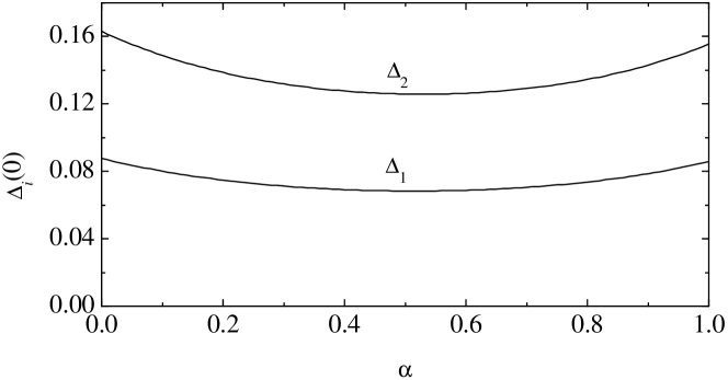
Figure 5: Plot of the normal stress differences $\Delta_{1}=(P_{zz}-P_{xx})/{p}$ and $\Delta_{2}=(P_{zz}-P_{yy})/{p}$, evaluated at $y=0$, versus $\alpha$ for $g\lambda_{0}/v_{0}^{2}=0.05$.

V Concluding remarks

In this paper we have carried out a kinetic theory study of the steady planar Poiseuille flow undergone by a dilute granular gas under the action of the acceleration of gravity. In order to compensate locally for the energy loss due to the inelasticity of collisions, an external energy input in the form of a white noise driving has been assumed. This type of driving mechanism has been introduced in the literature to mimic the heating effects due vibrating boundaries without the complications associated with boundary effects. This is especially convenient in our approach, since we have been mainly interested in the bulk properties of the gas, namely in a slab centered in the middle layer having a width of the order of several mean free paths, away from the walls.

Since granular gases are made of mesoscopic particles, terrestrial gravity ($g=9.8~{}\text{m/s${}^{2}$}$) plays in general a relevant role, in contrast to the case of molecular gases. The dimensionless parameter characterizing the influence of gravity during the free flight of a particle between two successive collisions is $g\lambda/v_{\text{th}}^{2}$, where $\lambda$ is the mean free path and $v_{\text{th}}$ is a typical (thermal) velocity. Under many conditions of practical interest, the parameter $g\lambda/v_{\text{th}}^{2}$ can have a non-negligible effect and yet be sufficiently small as to justify a perturbative treatment. For instance, if $\lambda\sim 1~{}\text{mm}\text{--}1~{}\text{cm}$ and $v_{\text{th}}\gtrsim 1~{}\text{m/s}$, which are typical values in experiments on metallic or glass spheres, one can have $g\lambda/v_{\text{th}}^{2}\sim 10^{-3}\text{--}10^{-1}$. Therefore, in our study we have performed a perturbation expansion of the velocity distribution function in powers of the gravity strength through second order. The reference state (i.e., the state at zero gravity) is the steady uniform state heated by a white noise thermostat. Since the Boltzmann equation for inelastic spheres is quite complicated to deal with, we have employed a kinetic model equation inspired in the BGK model. This has allowed us to obtain explicitly the velocity distribution function through second order in terms of the velocity vector, the spatial coordinate, and the coefficient of restitution. By velocity integration one can obtain any desired moment, but here we have focused on the hydrodynamic fields (pressure, flow velocity, and granular temperature) and their associated fluxes (stress tensor and heat flux vector).

The results show that the non-Newtonian features previously studied in the case of elastic particlesTS94 ; TSS98 ; TS01 ; STS03 ; RC98 ; HM99 ; ATN02 persist when inelasticity is present. In particular, the temperature profile $T(y)$ exhibits a bimodal shape: it has a local minimum $T_{0}$ at the central layer and reaches two symmetric maxima $T_{\text{max}}$ at a distance $|y_{\text{max}}|$ of about three mean free paths. The relative height of the two maxima, $(T_{\text{max}}-T_{0})/T_{0}$ is about 10 times the square of the dimensionless parameter $g\lambda/v_{\text{th}}^{2}$. On the other hand, the heat flows outward from the central layer, so it goes from the colder to the hotter layers within the region $|y|<|y_{\text{max}}|$. Other non-Newtonian effects include normal stress differences and the existence of a component of the heat flux parallel to the flow and hence normal to the thermal gradient.

The fact that the nonlinear transport properties of the granular Poiseuille flow are qualitatively similar to those of the elastic case does not come as a surprise, especially since the characteristic collisional cooling of the granular gas is balanced by an external driving. In that context, our aim in the present work has been two-fold. On the one hand, the example of gravity-driven Poiseuille flow allows one to emphasize once more that granular gases constitute an excellent playground to reveal interesting (and even counter-intuitive) non-Newtonian phenomena on scales accessible to laboratory conditions. More importantly, we wanted to assess the influence of inelasticity on the departure of the Poiseuille profiles from the Navier–Stokes predictions. This influence is not easy to foretell a priori by means of intuitive or hand-waving arguments. According to the results reported in this paper, for small or moderate inelasticity (say $\alpha\gtrsim 0.5$) there is a slight decrease in the quantitative deviations from the Navier–Stokes profiles as inelasticity grows: the two temperature maxima becomes lower and closer, while the normal stress differences become smaller. The opposite behavior takes place for high inelasticity ($\alpha\lesssim 0.5$), although that range is less interesting from an experimental point of view.

Appendix A Expressions for the coefficients $b_{i}$, $c_{i}$, and $d_{i}$

In this Appendix we list the explicit expressions of the coefficients in the expression for the velocity distribution function to order $g^{2}$, Eq. (76). They are

$$b_{0}=-\frac{4}{5}\frac{(2+5\zeta_{0}^{*})(5+7{\zeta_{0}^{*}}+6{\zeta_{0}^{*}}^{2})}{(1+\zeta_{0}^{*})^{2}(2+\zeta_{0}^{*})(1+2\zeta_{0}^{*})(2+3\zeta_{0}^{*})},$$ (98)

$$b_{1}=\frac{8}{25}\frac{160+622\zeta_{0}^{*}-1051{\zeta_{0}^{*}}^{2}-2829{\zeta_{0}^{*}}^{3}-1696{\zeta_{0}^{*}}^{4}-276{\zeta_{0}^{*}}^{5}}{(1+\zeta_{0}^{*})^{2}(2+\zeta_{0}^{*})^{2}(2+7\zeta_{0}^{*}+6{\zeta_{0}^{*}}^{2})},$$ (99)

$$b_{2}=-\frac{48}{5}\frac{1+3\zeta_{0}^{*}}{(1+\zeta_{0}^{*})(2+\zeta_{0}^{*})(2+3\zeta_{0}^{*})},\quad b_{3}=0,$$ (100)

$$b_{4}=-\frac{32}{5}\frac{5+29\zeta_{0}^{*}+12{\zeta_{0}^{*}}^{2})}{(1+\zeta_{0}^{*})(2+\zeta_{0}^{*})(1+2\zeta_{0}^{*})(2+3\zeta_{0}^{*})},$$ (101)

$$b_{5}=\frac{32}{5}\frac{(5+2\zeta_{0}^{*})(1+3\zeta_{0}^{*})}{(1+\zeta_{0}^{*})(2+\zeta_{0}^{*})(2+3\zeta_{0}^{*})},\quad b_{6}=-\frac{16}{5}\frac{{\zeta_{0}^{*}}}{1+\zeta_{0}^{*}},\quad b_{7}=-\frac{8}{3},$$ (102)

$$c_{0}=8\frac{4+12\zeta_{0}^{*}+113{\zeta_{0}^{*}}^{2}+176{\zeta_{0}^{*}}^{3}+79{\zeta_{0}^{*}}^{4}+6{\zeta_{0}^{*}}^{5}}{(1+\zeta_{0}^{*})^{2}(2+\zeta_{0}^{*})^{2}(1+2\zeta_{0}^{*})(2+3\zeta_{0}^{*})},$$ (103)

$$c_{1}=-32\frac{(3+2\zeta_{0}^{*})(2-11\zeta_{0}^{*}-12{\zeta_{0}^{*}}^{2})}{(1+\zeta_{0}^{*})^{2}(2+\zeta_{0}^{*})^{2}(1+2\zeta_{0}^{*})(2+3\zeta_{0}^{*})},$$ (104)

$$c_{2}=16\frac{8-22\zeta_{0}^{*}-23{\zeta_{0}^{*}}^{2}-3{\zeta_{0}^{*}}^{3}}{(1+\zeta_{0}^{*})(2+\zeta_{0}^{*})^{2}(2+3\zeta_{0}^{*})},\quad c_{3}=8\frac{{\zeta_{0}^{*}}}{1+\zeta_{0}^{*}},$$ (105)

$$c_{4}=64\frac{3+2\zeta_{0}^{*}}{(1+\zeta_{0}^{*})(2+\zeta_{0}^{*})(1+2\zeta_{0}^{*})(2+3\zeta_{0}^{*})},$$ (106)

$$c_{5}=-64\frac{3+2\zeta_{0}^{*}}{(1+\zeta_{0}^{*})(2+\zeta_{0}^{*})(2+3\zeta_{0}^{*})},\quad c_{6}=\frac{16}{1+{\zeta_{0}^{*}}},$$ (107)

$$d_{0}=\frac{8}{25}{\zeta_{0}^{*}}\frac{76-48\zeta_{0}^{*}-137{\zeta_{0}^{*}}^{2}+7{\zeta_{0}^{*}}^{3}+42{\zeta_{0}^{*}}^{4}}{(1+\zeta_{0}^{*})^{2}(2+\zeta_{0}^{*})^{2}(1+2\zeta_{0}^{*})(2+3\zeta_{0}^{*})},$$ (108)

$$d_{1}=\frac{16}{25}\frac{76-48\zeta_{0}^{*}-137{\zeta_{0}^{*}}^{2}+7{\zeta_{0}^{*}}^{3}+42{\zeta_{0}^{*}}^{4}}{(1+\zeta_{0}^{*})^{2}(2+\zeta_{0}^{*})^{2}(1+2\zeta_{0}^{*})(2+3\zeta_{0}^{*})},$$ (109)

$$d_{2}=-\frac{16}{25}\frac{76+40\zeta_{0}^{*}+23{\zeta_{0}^{*}}^{2}+21{\zeta_{0}^{*}}^{3}}{(1+\zeta_{0}^{*})(2+\zeta_{0}^{*})^{2}(2+3\zeta_{0}^{*})},\quad d_{3}=-\frac{8}{5}\frac{{\zeta_{0}^{*}}}{1+\zeta_{0}^{*}},$$ (110)

$$d_{4}=-\frac{64}{5}\frac{1}{(1+\zeta_{0}^{*})(1+2\zeta_{0}^{*})(2+3\zeta_{0}^{*})},$$ (111)

$$d_{5}=\frac{64}{5}\frac{1}{(1+\zeta_{0}^{*})(2+3\zeta_{0}^{*})},\quad d_{6}=-\frac{16}{5}\frac{1}{1+\zeta_{0}^{*}},\quad d_{7}=\frac{16}{15}.$$ (112)

References

- (1) D. J. Tritton, Physical Fluid Dynamics (Oxford University Press, Oxford, 1988); G. K. Batchelor, An Introduction to Fluid Dynamics (Cambridge University Press, Cambridge, 1967); R. B. Bird, W. E. Stewart, and E. W. Lightfoot, Transport Phenomena (Wiley, New York, 1960); H. Lamb, Hydrodynamics (Dover, New York, 1945).
- (2) L. P. Kadanoff, G. R. McNamara, and G. Zanetti, A Poiseuille viscometer for lattice gas automata, Complex Syst. 1:791–803 (1987); From automata to fluid flow: Comparison of simulation and theory, Phys. Rev. A 40:4527–4541 (1989).
- (3) M. Alaoui and A. Santos, Poiseuille flow driven by an external force, Phys. Fluids A 4:1273–1282 (1992).
- (4) R. Esposito, J. L. Lebowitz, and R. Marra, A hydrodynamic limit of the stationary Boltzmann equation in a slab, Commun. Math. Phys. 160:49–80 (1994).
- (5) M. Tij and A. Santos, Perturbation analysis of a stationary nonequilibrium flow generated by an external force, J. Stat. Phys. 76:1399–1414 (1994). Note a misprint in Eq. (59): the denominators 25, 30, 3125, 750 and 250 should be multiplied by 3, 5, 3, 5 and 7, respectively.
- (6) K. P. Travis, B. D. Todd, and D. J. Evans, Poiseuille flow of molecular fluids, Physica A 240:315–327 (1997); B. D. Todd and D. J. Evans, Temperature profile for Poiseuille flow, Phys. Rev. E 55:2800–2807 (1997); G. Ayton, O. G. Jepps, and D. J. Evans, On the validity of Fourier’s law in systems with spatially varying strain rates, Mol. Phys. 96:915–920 (1999).
- (7) M. Malek Mansour, F. Baras, and A. L. Garcia, On the validity of hydrodynamics in plane Poiseuille flows, Physica A 240:255–267 (1997).
- (8) M. Tij, M. Sabbane, and A. Santos, Nonlinear Poiseuille flow in a gas, Phys. Fluids 10:1021–1027 (1998).
- (9) D. Risso and P. Cordero, Generalized hydrodynamics for a Poiseuille flow: theory and simulations, Phys. Rev. E 58:546–553 (1998).
- (10) F. J. Uribe and A. L. Garcia, Burnett description for plane Poiseuille flow, Phys. Rev. E 60:4063–4078 (1999).
- (11) S. Hess and M. Malek Mansour, Temperature profile of a dilute gas undergoing a plane Poiseuille flow, Physica A 272:481–496 (1999).
- (12) P. Cordero and D. Risso, Nonlinear effects in gases due to strong gradients, in Rarefied Gas Dynamics: 22nd International Symposium, edited by T. J. Bartel and M. A. Gallis (American Institute of Physics, 2001).
- (13) M. Tij and A. Santos, Non-Newtonian Poiseuille flow of a gas in a pipe, Physica A 289:336–358 (2001).
- (14) K. Aoki, S. Takata, and T. Nakanishi, A Poiseuille-type flow of a rarefied gas between two parallel plates driven by a uniform external force, Phys. Rev. E 65:026315 (2002).
- (15) Y. Zheng, A. L. Garcia, and B. J. Alder, Comparison of kinetic theory and hydrodynamics for Poiseuille flow, J. Stat. Phys. 109:495–505 (2002).
- (16) M. Sabbane, M. Tij, and A. Santos, Maxwellian gas undergoing a stationary Poiseuille flow in a pipe, Physica A 327:264–290 (2003).
- (17) J. O. Hischfelder, C. F. Curtiss, and R. B. Bird, Molecular Theory of Gases and Liquids (Wiley, New York, 1964), p. 15.
- (18) C. S. Campbell, Rapid granular flows, Annu. Rev. Fluid Mech. 22:57–92 (1990).
- (19) H. M. Jaeger and S. R. Nagel, Granular solids, liquids, and gases, Rev. Mod. Phys. 68:1259–1273 (1996).
- (20) L. P. Kadanoff, Built upon sand: Theoretical ideas inspired by granular flows, Rev. Mod. Phys. 71:435–444 (1996).
- (21) I. Goldhirsch, Scales and kinetics of granular flows, Chaos 9:659–672 (1999); Rapid granular flows, Annu. Rev. Fluid Mech. 35:267–293 (2003).
- (22) J. W. Dufty, Statistical mechanics, kinetic theory, and hydrodynamics for rapid granular flow, J. Phys.: Condens. Matt. 12:A47–A56 (2000); Kinetic theory and hydrodynamics for rapid granular flow — A perspective, Recent Res. Devel. Stat. Phys. 2:21–52 (2002), e-print cond-mat/0108444; Kinetic theory and hydrodynamics for a low density granular gas, Adv. Compl. Syst. 4:397–406 (2001); reprinted in Challenges in Granular Physics, T. Halsey and A. Mehta, eds. (World Scientific, Singapore, 2002), pp. 109–118.
- (23) N. Brilliantov and T. Pöschel, Kinetic Theory of Granular Gases (Oxford University Press, Oxford, 2004).
- (24) D. L. Blair and A. Kudrolli, Velocity correlations in dense granular gases, Phys. Rev. E 64:050301(R) (2001).
- (25) W. Losert, D. G. W. Cooper, J. Delour, A. Kudrolli, and J. P. Gollub, Velocity statistics in excited granular media, Chaos 9:682–690 (1999).
- (26) E. Falcon, R. Wunenburger, P. Évesque, S. Fauve, C. Chabot, Y. Garrabos, and D. Beysens, Cluster formation in a granular medium fluidized by vibrations in low gravity, Phys. Rev. Lett. 83:440–443 (1999).
- (27) J. J. Brey, J. W. Dufty, and A. Santos, Kinetic models for granular flow, J. Stat. Phys. 97:281–322 (1999).
- (28) C. Cercignani, The Boltzmann Equation and Its Applications (Springer–Verlag, New York, 1988).
- (29) A. Goldshtein and M. Shapiro, Mechanics of collisional motion of granular materials. Part 1. General hydrodynamic equations, J. Fluid Mech. 282:75–114 (1995).
- (30) J. J. Brey, J. W. Dufty, and A. Santos, Dissipative dynamics for hard spheres, J. Stat. Phys. 87:1051–1066 (1997).
- (31) J. J. Brey, J. W. Dufty, C. S. Kim, and A. Santos, Hydrodynamics for granular flow at low density, Phys. Rev. E 58:4638–4653 (1998).
- (32) D. R. M. Williams and F. C. MacKintosh, Driven granular media in one dimension: correlations and equation of state, Phys. Rev. E 54:R9–R12 (1996); D. R. M. Williams, Driven granular media and dissipative gases: correlations and liquid-gas phase transitions, Physica A 233:718–729 (1996).
- (33) T. P. C. van Noije and M. H. Ernst, Velocity distributions in homogeneous granular fluids: the free and the heated case, Gran. Matt. 1:57–64 (1998).
- (34) M. R. Swift, M. Boamfǎ, S. J. Cornell, and A. Maritan, Scale invariant correlations in a driven dissipative gas, Phys. Rev. Lett., 80:4410–4413 (1998).
- (35) T. P. C. van Noije, M. H. Ernst, E. Trizac, and I. Pagonabarraga, Randomly driven granular fluids: Large-scale structure, Phys. Rev. E 59:4326–4341 (1999); I. Pagonabarraga, E. Trizac, T. P. C. van Noije, and M. H. Ernst, Randomly driven granular fluids: collisional statistics and short scale structure, Phys. Rev. E 65:011303 (2002).
- (36) C. Bizon, M. D. Shattuck, J. B. Swift, and H. L. Swinney, Transport coefficients for granular media from molecular dynamics simulations, Phys. Rev. E 60:4340–4351 (1999).
- (37) J. M. Montanero and A. Santos, Computer simulation of uniformly heated granular fluids, Gran. Matt. 2:53–64 (2000).
- (38) E. Ben-Naim and P. L. Krapivsky, Multiscaling in inelastic collisions, Phys. Rev. E 61:R5-R8 (2000); P. Krapivsky and E. Ben-Naim, Nontrivial velocity distributions in inelastic gases, J. Phys. A: Math. Gen. 35:L147–L152 (2002).
- (39) J. A. Carrillo, C. Cercignani, and I. M. Gamba, Steady states of a Boltzmann equation for driven granular media, Phys. Rev. E 62:7700–7707 (2000).
- (40) V. Garzó and J. W. Dufty, Dense fluid transport for inelastic hard spheres, Phys. Rev. E 59:5895–5911 (1999).
- (41) V. Garzó and J.M. Montanero, Transport coefficients of a heated granular gas, Physica A 313:336–356 (2002).
- (42) A. Santos, Transport coefficients of -dimensional inelastic Maxwell models, Physica A, 321: 442–466 (2003).
- (43) A. Santos and A. Astillero, Can a system of elastic hard spheres mimic the transport properties of a granular gas?, e-print cond-mat/0405252.
- (44) J. J. Brey, M. J. Ruiz–Montero, and F. Moreno, Steady uniform shear flow in a low density granular gas, Phys. Rev. E, 55:2846–2856 (1997).
- (45) J. M. Montanero, V. Garzó, A. Santos, and J. J. Brey, Kinetic theory of simple granular shear flows of smooth hard spheres, J. Fluid Mech. 389:391–411 (1999).
- (46) M. Tij, E. E. Tahiri, J. M. Montanero, V. Garzó, A. Santos, and J.W. Dufty, Nonlinear Couette flow in a low density granular gas, J. Stat. Phys. 103:1035–1068 (2001). Note a misprint below Eq. (26): should be replaced by .