Transfer matrix and Monte Carlo tests of critical exponents in Ising model

Abstract

The corrections to finite-size scaling in the critical two-point correlation function $G(r)$ of 2D Ising model on a square lattice have been studied numerically by means of exact transfer–matrix algorithms. The systems have been considered, including up to 800 spins. The calculation of $G(r)$ at a distance $r$ equal to the half of the system size $L$ shows the existence of an amplitude correction $\propto L^{-2}$. A nontrivial correction $\propto L^{-0.25}$ of a very small magnitude also has been detected, as it can be expected from our recently developed GFD (grouping of Feynman diagrams) theory. Monte Carlo simulations of the squared magnetization of 3D Ising model have been performed by Wolff’s algorithm in the range of the reduced temperatures $t\geq 0.000086$ and system sizes $L\leq 410$. The effective critical exponent $\beta_{eff}(t)$ tends to increase above the currently accepted numerical values. The critical coupling $K_{c}=0.22165386(51)$ has been extracted from the Binder cumulant data within $L\in[96;384]$. The critical exponent $1/\nu$, estimated from the finite–size scaling of the derivatives of the Binder cumulant, tends to decrease slightly below the RG value $1.587$ for the largest system sizes. The finite–size scaling of accurately simulated maximal values of the specific heat $C_{V}$ in 3D Ising model confirms a logarithmic rather than power–like critical singularity of $C_{V}$.

Keywords: Transfer matrix, Ising model, $\varphi^{4}$ model, critical exponents, finite–size scaling, Monte Carlo simulation

Pacs: 64.60.Cn, 68.18.Jk, 05.10.-a

1 Introduction

Since the exact solution of two–dimensional Lenz–Ising (or Ising) model has been found by Onsager [1], a study of various phase transition models is of permanent interest. Nowadays, phase transitions and critical phenomena is one of the most widely investigated fields of physics [2, 3]. Remarkable progress has been reached in exact solution of two–dimensional models [4]. Recently, we have proposed [5] a novel method based on grouping of Feynman diagrams (GFD) in $\varphi^{4}$ model. Our GFD theory allows to analyze the asymptotic solution for the two–point correlation function at and near criticality, not cutting the perturbation series. As a result the possible values of exact critical exponents have been proposed [5] for the Ginzburg–Landau ($\varphi^{4}$) model with $O(n)$ symmetry, where $n=1,2,3,\ldots$ is the dimensionality of the order parameter. Our predictions completely agree with the known exact and rigorous results in two dimensions [4]. In [5], we have compared our results to some Monte Carlo (MC) simulations and experiments [6, 7, 8]. The examples considered there support our predictions about the critical exponents. A more recent comparison with experimental data very close to the $\lambda$–transition point $T=T_{\lambda}$ in liquid helium has been made in [9]. We have shown there that our critical exponents better describe the closest to $T_{\lambda}$ data for the superfluid fraction of liquid helium as compared to the exponents provided by the perturbative renormalization group (RG) theory [10, 11, 12]. As claimed in [5], the conventional RG expansions are not valid from the mathematical point of view. The current paper, dealing with numerical transfer-matrix analysis of the two–point correlation function in 2D Ising model, as well as with MC simulations in the three–dimensional Ising model presents some more evidences in favour of the critical exponents predicted by the GFD theory. Our estimations are based on the finite–size scaling theory, which by itself is an attractive field of investigations [13] and has increasing importance in modern physics [3].

2 Critical exponents predicted by GFD theory

Our theory predicts possible values of exact critical exponents $\gamma$ and $\nu$ for the $\varphi^{4}$ model whith $O(n)$ symmetry ($n$–component vector model) given by the Hamiltonian

$$H/T=\int\left[r_{0}\varphi^{2}({\bf x})+c(\nabla\varphi({\bf x}))^{2}+u\varphi^{4}({\bf x})\right]d{\bf x}\;,$$ (1)

where $r_{0}$ is the only parameter depending on temperature $T$, and the dependence is linear. At the spatial dimensionality $d=2,3$ and $n=1,2,3,...$ the predicted possible values of the critical exponents are [5]

$$\gamma = \frac{d+2j+4m}{d(1+m+j)-2j}\;,$$ (2)

$$\nu = \frac{2(1+m)+j}{d(1+m+j)-2j}\;,$$ (3)

where $m\geq 1$ and $j\geq-m$ are integers. It is well known that the $O(n)$–symmetric $\varphi^{4}$ model belongs to the same universality class as the corresponding lattice model (Ising model at $n=1$, $XY$ model at $n=2$, the classical Heisenberg model at $n=3$, etc.), where the order parameter is an $n$-component vector (spin) with fixed modulus $\mid\varphi({\bf x})\mid=1$, since the latter is a particular case ($r_{0}\to-\infty$ at $-r_{0}/(2u)=1$ or $\lambda\to\infty$ in the notations used in [14]) of the lattice $\varphi^{4}$ model, where the gradient term is represented by finite differences [14]. Besides, the partition functions and two–point correlation functions of both $\varphi^{4}$ model in [5] and Ising model can be represented by similar functional integrals [15, 16]. Thus, at $n=1$ we have $m=3$ and $j=0$ to fit the known exact results for the two–dimensional Ising model. As proposed in Ref. [5], in the case of $n=2$ we have $m=3$ and $j=1$, which yields in three dimensions $\nu=9/13$ and $\gamma=17/13$.

As already explained in [5], our predictions do not refer to the case of the self–avoiding random walk recovered at $n=0$. The values (2) and (3) have been derived in [5] assuming that $2\nu-\gamma>0$ holds. In principle, the mean–field–like solution with $2\nu-\gamma=0$ can exist at $d<4$, and it refers to the Gaussian random walk with $n=-2$. This is a special case, not related to (2) and (3), where two expansion parameters $\Delta^{2\nu-\gamma}$ and $\Delta^{2\gamma-d\nu}$ with $\Delta=T-T_{c}\to 0$ being the deviation from the critical temperature $T_{c}$, are replaced by one parameter $\Delta^{2\gamma-d\nu}$. Eq. (48) in [5] can be then satisfied with $\gamma=1$ and $\nu=1/2$, i. e., all the exponents are consistent and each term can be compensated. The singularity of the specific heat with the exponent $\alpha=2-d/2$ comes from the leading terms in Eq. (60) of [5]. Obviously, $\gamma=1$ and $\nu=1/2$ always are the true exponents at $d>4$, where the Gaussian approximation $G({\bf k})=1/\left[G({\bf 0})^{-1}+2ck^{2}\right]$ for the two-point correlation function $G({\bf k})$ in the Fourier representation is asymptotically exact at $u\to 0$ and $T>T_{c}$ for arbitrarily small wave vectors ${\bf k}$. These exponents are recovered at any $m$ and $j$ in (2) and (3) when approaching the upper critical dimension $d=4$ from below.

Our formulae do not provide any sensible result approaching $d=1$, where $\nu=1/(d-1)$ is expected at $n=1$ according to the Midgal’s approximation [17]. It can be understood from the point of view [18] that $2$, probably, is the marginal value of $d$, such that an analytic continuation of the results from $d$-dimensional hypercubes can be only formal and has no physical meaning at $d<2$. In this sense, we expect that $d=2$ is a special dimension for any $n\geq 1$. Besides, the critical temperature does not vanish at $d\to 2+0$, and for $n=1$ there exist lattices for which the critical temperature is nonzero at the fractal dimension below 2 [19]. In the marginal case $d=2$ different behavior is observed at low temperatures: the long–range order at $n=1$, the Kosterlitz–Thouless structural order at $n=2$, and disordered state at $n>2$.

Our concept agrees with the known rigorous results for $XY$ model [20, 21]. It disagrees with the prediction of the perturbative RG theory [22] that the critical temperature goes to zero at $d\to 2+0$ for the $O(n>2)$–symmetric nonlinear $\sigma$ model and, therefore, the behavior in this case is Gaussian, i. e., $\eta=0$ and $\nu=1/(d-2)$. The results of the perturbative RG theory are not rigorous since the claims are based on formal expansions which break down in relevant limits, in this case at vanishing external field $H\to+0$. Moreover, essential claims of this theory are based on an evidently incorrect mathematical treatment. In particular, the conclusion about the Gaussian character of the $O(n)$–symmetric $\varphi^{4}$ model below $T_{c}$ has been made in [23] by simply rewritting the Hamiltonian in an apparently Gaussian form (see Eqs. (3.4) to (3.6) in [23]). The author, however, forgot to include the determinant of the transformation Jacobian in the relevant functional integrals, according to which the resulting model all the same is not Gaussian. Due to the reasons mentioned above, we do not believe in predictions of the perturbative RG theory, but rely only on exact and rigorous results.

There exists a simple non–perturbative explanation why the critical temperature should stay finite at $d\to 2+0$ for the $O(n)$–symmetric Heisenberg model. Below $T_{c}$, the difference in free energies for models with antiperiodic and periodic boundary conditions along one axis is $\Delta F\propto\Upsilon(T)L^{d-2}$, where $L$ is the linear size of the system and $\Upsilon(T)$ is the helicity modulus. It holds because the energy difference in the ground state at $T=0$ is $\propto L^{d-2}$, corresponding to gradually rotated spins in any given plane. The factor $\Upsilon(T)$ takes into account the temperature dependence. It vanishes at $T\geq T_{c}$. Hence, the factor $L^{d-2}$ always vanishes at $d<2$ in the thermodynamic limit $L\to\infty$, therefore the long–range order (if it would exist) could be destroyed in this case at any finite temperature by gradually rotating the spins without increasing the free energy. Thus, the long–range order disappears at $d<2$ irrespective to the behavior of $\Upsilon(T)$, i. e., irrespective to the value of $T_{c}$ at $d=2+0$. In such a way, the assumption that the critical temperature should go to zero continuously appears as an additional unnecessary constraint. On the other hand, if the critical temperature remains finite in $\varphi^{4}$ model, then $\eta$ should be positive at $d=2+0$ to avoid the divergence of $\langle\varphi^{2}({\bf x})\rangle=n\,L^{-d}\sum_{\bf k}G({\bf k})$ at $T=T_{c}$, where $G({\bf k})\simeq a\,k^{-2+\eta}$ with $a\neq 0$ holds for the two–point correlation function. The expectation $\eta>0$ agrees with (2) and (3). However, the critical temperature at $d=2+0$ and $\eta$ tend to zero in the limit $n\to\infty$ to coincide with the known exact results for the spherical model, which are recovered in (2) and (3) at $j/m\to\infty$.

In the present analysis the correction–to–scaling exponent $\theta$ for the susceptibility is also relevant. The susceptibility is related to the correlation function $G({\bf k})$ via $\chi\propto G({\bf 0})$ [11]. In the thermodynamic limit, this relation makes sense at $T>T_{c}$. According to our theory, $t^{\gamma}G({\bf 0})$ can be expanded in a Taylor series of $t^{2\nu-\gamma}$ at $t\to 0$. In this case the reduced temperature $t$ is defined as $t=r_{0}(T)-r_{0}(T_{c})\propto T-T_{c}$. Formally, $t^{2\gamma-d\nu}$ appears as second expansion parameter in the derivations in Ref. [5], but, according to the final result represented by Eqs. (2) and (3), $(2\gamma-d\nu)/(2\nu-\gamma)$ is a natural number. Some of the expansion coefficients can be zero, so that in general we have

$$\theta=\ell\,(2\nu-\gamma)\;,$$ (4)

where $\ell$ may have integer values 1, 2, 3, etc. One can expect that $\ell=4$ holds at $n=1$ (which yields $\theta=1$ at $d=2$ and $\theta=1/3$ at $d=3$) and the only nonvanishing corrections are those of the order $t^{\theta}$, $t^{2\theta}$, $t^{3\theta}$, since the known corrections to scaling for physical quantities, such as magnetization or correlation length, are analytical in the case of the two–dimensional Ising model. Here we suppose that the confluent corrections become analytical, i. e. $\theta$ takes the value $1$, at $d=2$. Besides, similar corrections to scaling are expected for susceptibility $\chi$ and magnetization $M$ since both these quantities are related to $G({\bf 0})$, i. e., $\chi\propto G({\bf 0})$ and $M^{2}=\lim_{x\to\infty}\langle\varphi({\bf 0})\varphi({\bf x})\rangle=\lim_{V\to\infty}G({\bf 0})/V$ hold where $V=L^{d}$ is the volume and $L$ is the linear size of the system. The above limit is meaningful at $L\to\infty$, but $G({\bf 0})/V$ may be considered as a definition of $M^{2}$ for finite systems too. The latter means that corrections to finite–size scaling for $\chi$ and $M$ are similar at $T=T_{c}$. According to the scaling hypothesis and finite–size scaling theory, the same is true for the discussed here corrections at $t\to 0$, where in both cases ($\chi$ and $M$) the definition $t=\mid r_{0}(T)-r_{0}(T_{c})\mid$ is valid. Thus, the expected expansion of the susceptibility $\chi$ looks like $\chi=t^{-\gamma}\left(a_{0}+a_{1}t^{\theta}+a_{2}t^{2\theta}+\cdots\right)$. In this discussion we have omitted the irrelevant for critical behaviour background term in the susceptibility, which is constant in the first approximation and comes from the short–distance contribution to $\chi=\sum_{\bf x}G({\bf x})$ [11], where $G({\bf x})$ is the real–space two–point correlation function.

Our hypothesis is that $j=j(n)$ and $\ell=\ell(n)$ monotoneously increase with $n$ to fit the known exponents for the spherical model at $n\to\infty$. The analysis of the MC and experimental results here and in [5] enables us to propose that $j(n)=n-1$, $\ell(n)=n+3$, and $m=3$ hold at least at $n=1,2,3$. These relations, probably, are true also at $n>3$. This general hypothesis is consistent with the idea that the critical exponents $\gamma$, $\nu$, and $\theta$ can be represented by some analytical functions of $n$ which are valid for all natural positive $n$ and yield $\eta=2-\gamma/\nu\propto 1/n$ rather than $\eta\propto 1/n^{s}$ with $s=2,3,\ldots$ ($s$ must be a natural number to avoid a contradiction, i. e., irrational values of $j(n)$ at natural $n$) at $n\to\infty$. At these conditions, $j(n)$ and $\ell(n)$ are linear functions of $n$ (with integer coefficients) such that $\ell(n)/j(n)\to 1$ at $n\to\infty$, and $m$ is constant. Besides, $j(1)=0$, $m(1)=3$, and $\ell(1)=4$ hold to coincide with the known results at $n=1$. Then, our specific choice is the best one among few possibilities providing more or less reasonable agreement with the actually discussed numerical an experimental results.

We allow that different $\ell$ values correspond to the leading correction–to–scaling exponent for different quantities related to $G({\bf k})$. According to [5], the expansion of $G({\bf k})$ in $\varphi^{4}$ model by itself contains a nonvanishing term of order $t^{2\nu-\gamma}\equiv t^{\eta\nu}$ (in the form $G({\bf k})\simeq t^{-\gamma}\left[g({\bf k}t^{-\nu})+t^{\eta\nu}g_{1}({\bf k}t^{-\nu})\right]$ whith $g_{1}({\bf 0})=0$, since $\ell>1$ holds in the case of susceptibility) to compensate the corresponding correction term (produced by $c\left(\nabla\varphi\right)^{2}$) in the equation for $1/G({\bf k})$ (cf. [5]).

The correction $t^{\eta\nu}$ is related to correction term $x^{-\eta}$ in the long–distance ($x\to\infty$) behavior of the real–space pair correlation function $G(x)\propto x^{2-d-\eta}\left[1+\mathcal{O}\left(x^{-\eta}\right)\right]$ at the critical point, as well as to correction $L^{-\eta}$ in the finite–size scaling expressions at criticality. Such kind of corrections must not necessarily appear in the Ising model, where they could have zero amplitude. In particular, the critical Green’s (correlation) function $G(x)$ of 2D Ising model in $\langle 11\rangle$ crystallographic direction on an infinite lattice can be calculated easily based on the known exact formulae [24], and it yields $G(x)\propto x^{-1/4}\left[1+\mathcal{O}\left(x^{-2}\right)\right]$ at large distances $x\to\infty$. Nevertheless, our calculations in 2D Ising model discussed in Sec. 4.3 indicate the existence of a nontrivial finite–size correction of the kind $L^{-\eta}$ (for $\langle 10\rangle$ direction), as it can be expected from our theoretical results for the $\varphi^{4}$ model. The thermodynamic limit is a particular case of the finite–size scaling with the scaling argument $x/L\to 0$, therefore it is possible that the nontrivial corrections to the correlation function in 2D Ising model vanish in this special case or in the crystallographic direction $\langle 11\rangle$, but not in general.

Our consideration can be generalized easily to the case where the Hamiltonian parameter $r_{0}$ is a nonlinear analytical function of $T$. Nothing is changed in the above expansions if the reduced temperature $t$, as before, is defined by $t=r_{0}(T)-r_{0}(T_{c})$. However, analytical corrections to scaling appear (and also corrections like$(T-T_{c})^{m+n\theta}$ with integer $m$ and $n$) if $t$ is reexpanded in terms of $T-T_{c}$ at $T>T_{c}$. The solution at the critical point remains unchanged, since the phase transition occurs at the same (critical) value of $r_{0}$.

3 Exact transfer matrix algorithms for calculation of the correlation function in 2D Ising model

3.1 Adoption of standard methods

The transfer matrix method, applied to analytical calculations on two–dimensional lattices, is well known [1, 4]. The asymptotic behavior of the correlation functions can be studied by means of the equations of the conformal field theory [25]. Exact equations for the two–point correlation function of 2D Ising model on an infinite lattice are known, too [24]. However, no analytical methods exist for an exact calculation of the correlation function in 2D Ising model on finite–size lattices. This can be done numerically by adopting the conventional transfer matrix method and modifying it to reach the maximal result (calculation of as far as possible larger system) with minimal number of arithmetic operations, as discussed further on.

We consider the two–dimensional Ising model where spins are located either on the lattice of dimensions $N\times L$, illustrated in Fig. 1a, or on the lattice of dimensions $\sqrt{2}N\times\sqrt{2}L$, shown in Fig. 1b. The periodic boundaries are indicated by dashed lines. In case (a) we have $L$ rows, and in case (b) – $2L$ rows, each containing $N$ spins. Fig. 1 shows an illustrative example with $N=4$ and $L=3$. In our notation nodes are numbered sequently from left to right, and rows – from bottom to top.

       

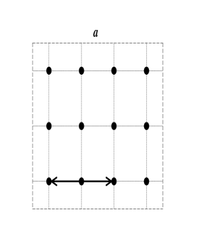
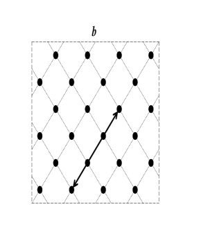
Figure 1: Illustrative examples of the lattices with dimensions $N\times L$ (a) and $\sqrt{2}N\times\sqrt{2}L$ (b) with periodic boundary conditions along the dashed lines. The correlation function has been calculated in the $\langle 10\rangle$ crystallographic direction, as indicated by the arrows.

For convenience, first we consider an application of the transfer matrix method to calculation of the partition function

$$Z=\sum\limits_{\{\sigma_{k}\}}\exp\left(\beta\sum\limits_{\langle i,j\rangle}\sigma_{i}\sigma_{j}\right)\;,$$ (5)

where $\sigma_{i}=\pm 1$ are the spin variables, and the summation runs over all the possible spin configurations $\{\sigma_{k}\}$. The argument of the exponent represents the Hamiltonian of the system including summation over all the neighbouring spin pairs $\langle i,j\rangle$ of the given configuration $\{\sigma_{k}\}$; parameter $\beta$ is the coupling constant. Let us consider lattice (a) in Fig. 1, but containing $n$ rows without periodic boundaries along the vertical axis and without interaction between spins in the upper row. We define the $2^{N}$–component vector ${\bf r}_{n}$ such that the $i$–th component of this vector represents the contribution to the partition function provided by the $i$–th spin configuration of the upper row. Then we have a recurrence relation ${\bf r}_{n+1}=T\,{\bf r}_{n}$, where $T$ is the transfer matrix which includes the Boltzmann weights of newly added bonds. Furthermore, we can write ${\bf r}_{n+1}^{(i)}=T\,{\bf r}_{n}^{(i)}$, where ${\bf r}_{n}^{(i)}$ is the partial contribution to ${\bf r}_{n}$ provided by the $i$–th configuration of the first row. The components of ${\bf r}_{1}^{(i)}$ are given by $\left({\bf r}_{1}^{(i)}\right)_{j}=\delta_{j,i}$. In the case of the periodic boundary conditions the $(L+1)$–th row must be identical to the first one, which leads to the well known expression [4, 26]

$$Z=\sum\limits_{i}\left({\bf r}_{L+1}^{(i)}\right)_{i}=\mbox{Trace}\left(T^{L}\right)=\sum\limits_{i}\lambda_{i}^{L}\;,$$ (6)

where $\lambda_{i}$ are the eigenvalues of the transfer matrix $T$. An analogous expression for the lattice in Fig. 1b reads

$$Z=\sum\limits_{i}\left({\bf r}_{2L+1}^{(i)}\right)_{i}=\mbox{Trace}\left(\left[T_{2}T_{1}\right]^{L}\right)\;,$$ (7)

where the vectors ${\bf r}_{n}^{(i)}$ obey the reccurence relation ${\bf r}_{n+1}^{(i)}=T_{1,2}\,{\bf r}_{n}^{(i)}$ with different transfer matrices $T_{1}$ and $T_{2}$ for odd and even row numbers $n$, respectively.

The actual scheme can be easily adopted to calculate the correlation function $\langle\sigma_{i}\sigma_{j}\rangle$ between any two lattice points $i$ and $j$. Namely, the correlation funtion $G(x)$ between the points separated by a distance $x$, like indicated in Fig. 1, is given by the statistical average $Z^{\prime}/Z$, where the sum $Z^{\prime}$ is calculated in the same way as $Z$, but including the corresponding product of spin variables. It implies the following replacements:

$$\left({\bf r}_{1}^{(i)}\right)_{j}=\delta_{j,i}\Rightarrow\left({\bf r}_{1}^{(i)}\right)_{j}=\delta_{j,i}\,\left(N^{-1}\sum\limits_{\ell=1}^{N}\left[\sigma(\ell)\right]_{i}\left[\sigma(\ell+x)\right]_{i}\right) :\mbox{case~{}(a)}$$ (8)

$$\left({\bf r}_{x+1}^{(i)}\right)_{j}\Rightarrow\left({\bf r}_{x+1}^{(i)}\right)_{j}\times\left(N^{-1}\sum\limits_{\ell=1}^{N}\left[\sigma(\ell)\right]_{i}\left[\sigma(\ell+\Delta(x))\right]_{j}\right) :\mbox{case~{}(b)}\;,$$ (9)

where $\Delta(x)=x/2$ holds for even $x$, and $\Delta(x)=(x-1)/2$ – for odd $x$. In our notation, $[\sigma(k)]_{i}$ is the spin variable in the $k$–th node in a row provided that the whole set of spin variables of this row forms the $i$–th configuration. It is supposed that $\sigma(k+N)\equiv\sigma(k)$ holds according to the periodic boundary conditions. Such a symmetrical form, which includes an averaging over $\ell$, allows to reduce the amount of numerical calculations: due to the symmetry we need the summation over only $\approx 2^{N}/N$ nonequivalent configurations of the first row instead of the total number of $2^{N}$ configurations.

3.2 Improved algorithms

The number of the required arithmetic operations can be further reduced if the recurrence relations ${\bf r}_{n+1}^{(i)}=T\,{\bf r}_{n}^{(i)}$ and ${\bf r}_{n+1}^{(i)}=T_{1,2}\,{\bf r}_{n}^{(i)}$ are split into $N$ steps of adding single spin. To formulate this in a suitable way, let us first number all the $2^{N}$ spin configurations $\{\sigma(1);\sigma(2);\cdots;\sigma(N-1);\sigma(N)\}$ by an index $i$ as follows:

$$\begin{array}[]{@{i \: = \:}l@{\hspace{2ex} : \hspace{3ex} \{}*{6}{c}@{\}}}\>=\>\lx@intercol 1\hfil\hskip 8.61108pt:\hskip 12.91663pt&-1;&-1;&\cdots;&-1;&-1;&-1\\ \>=\>\lx@intercol 2\hfil\hskip 8.61108pt:\hskip 12.91663pt&-1;&-1;&\cdots;&-1;&-1;&+1\\ \>=\>\lx@intercol 3\hfil\hskip 8.61108pt:\hskip 12.91663pt&-1;&-1;&\cdots;&-1;&+1;&-1\\ \>=\>\lx@intercol 4\hfil\hskip 8.61108pt:\hskip 12.91663pt&-1;&-1;&\cdots;&-1;&+1;&+1\\ \lx@intercol\dotfill\hfil\hfil\lx@intercol\\ \>=\>\lx@intercol 2^{N}\hfil\hskip 8.61108pt:\hskip 12.91663pt&+1;&+1;&\cdots;&+1;&+1;&+1\end{array}$$ (10)

We remind that the sequence of numbers in the $i$–th row corresponds to the spin variables $\left[\sigma(k)\right]_{i}$ with $k=1,2,\ldots,N$. They change with $i$ just like the digits of subsequent integer numbers in the binary counting system.

       

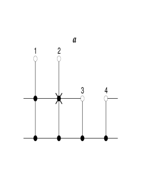
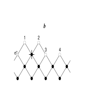
Figure 2: Schematic pictures illustrating the algorithms of calculation for the lattices $a$ and $b$ introduced in Fig. 1.

Consider now a lattice where $n$ rows are completed, while the $(n+1)$–th row contains only $\ell$ spins where $\ell<N$, as illustrated in Fig. 2 in both cases (a) and (b) taking as an example $N=4$. We consider the partial contribution $\left({\bf r}_{n+1,\ell}\right)_{i}$ (i. e., $i$–th component of vector ${\bf r}_{n+1,\ell}$) in the partition function $Z$ (or $Z^{\prime}$) provided by a fixed ($i$–th) configuration of the set of $N$ upper spins. These are the sequently numbered spins shown in Fig. 2 by empty circles. For simplicity, we have droped the index denoting the configuration of the first row. In case (b), the spin depicted by a double–circle has a fixed value $\sigma^{\prime}$. In general, this spin is the nearest bottom–left neighbour of the first spin in the upper row. According to this, one has to distinguish between odd and even $n$: $\sigma^{\prime}$ refers either to the first (for odd $n$), or to the $N$–th (for even $n$) spin of the $n$–th row. It is supposed that the Boltzmann weights are included corresponding to the solid lines in Fig. 2 connecting the spins. In case (a) the weights responsible for the interaction between the upper numbered spins are not included. Obviously, for a given $\ell>1$, ${\bf r}_{n+1,\ell}$ can be calculeted from ${\bf r}_{n+1,\ell-1}$ via summation over one spin variable, marked in Fig. 2 by a cross. In case (a) it is true also for $\ell=1$, whereas in case (b) this variable has fixed value $\sigma^{\prime}$ at $\ell=1$. In the latter case the summation over $\sigma^{\prime}$ is performed at the last step when the $(n+1)$–th row is already completed. These manipulations enable us to write

$${\bf r}_{n+1}=T\,{\bf r}_{n}\equiv\widetilde{W}_{N}\,\widetilde{W}_{N-1}\cdots\widetilde{W}_{2}\,\widetilde{W}_{1}\,{\bf r}_{n}$$ (11)

with

$$\widetilde{W}_{\ell}=\sum\limits_{\sigma=\pm 1}W_{\ell}(\sigma)\;,$$ (12)

where the componets of the matrices $W_{\ell}(\sigma)$ are given by

$$\left(W_{1}(\sigma)\right)_{ij} = \delta\left(j,j_{1}(\sigma,1,i)\right)\cdot\exp\left(\beta\,\sigma\left\{\left[\sigma(1)\right]_{i}+\left[\sigma(2)\right]_{i}+\left[\sigma(N)\right]_{i}\right\}\right)$$

$$\left(W_{\ell}(\sigma)\right)_{ij} = \delta\left(j,j_{1}(\sigma,\ell,i)\right)\cdot\exp\left(\beta\,\sigma\left\{\left[\sigma(\ell)\right]_{i}+\left[\sigma(\ell+1)\right]_{i}\right\}\right)\hskip 4.30554pt:\hskip 4.30554pt1<\ell<N$$

$$\left(W_{N}(\sigma)\right)_{ij} = \delta\left(j,j_{1}(\sigma,N,i)\right)\cdot\exp\left(\beta\,\sigma\left[\sigma(N)\right]_{i}\right)\;.$$ (13)

Here $\delta(j,k)$ is the Kronecker symbol and

$$j_{1}(\sigma,\ell,i)=i+\left(\sigma-\left[\sigma(\ell)\right]_{i}\right)\,2^{N-\ell-1}$$ (14)

are the indexes of the old configurations containing $\ell-1$ spins in the $(n+1)$–th row depending on the value $\sigma$ of the spin marked in Fig. 2a by a cross, as well as on the index $i$ of the new configuration with $\ell$ spins in the $(n+1)$–th row, as consistent with the numbering (10).

The above equations (11) to (13) refers to case (a). In case (b) we have

$${\bf r}_{n+1}=T_{1,2}\,{\bf r}_{n}\equiv\sum\limits_{\sigma^{\prime}=\pm 1}\widetilde{W}_{N}^{(1,2)}\,\widetilde{W}_{N-1}^{(1,2)}\cdots\widetilde{W}_{2}^{(1,2)}\,W_{1}^{(1,2)}(\sigma^{\prime})\,{\bf r}_{n}\;,$$ (15)

where $\widetilde{W}_{\ell}^{(1,2)}$ are the matrices

$$\widetilde{W}_{\ell}^{(1,2)}=\sum\limits_{\sigma=\pm 1}W_{\ell}^{(1,2)}(\sigma)\;.$$ (16)

Here indexes 1 and 2 refer to odd and even row numbers $n$, respectively, and the components of the matrices $W_{\ell}^{(1,2)}(\sigma)$ are

$$\left(W_{\ell}^{(1,2)}(\sigma)\right)_{ij}=\delta\left(j,j_{1,2}(\sigma,\ell,i)\right)\cdot\exp\left(\beta\left[\sigma(\ell)\right]_{i}\left\{\sigma+\left[\sigma(\ell+1)\right]_{i}\right\}\right)\;,$$ (17)

where $\left[\sigma(N+1)\right]_{i}\equiv\sigma^{\prime}$ and the index $j_{1}(\sigma,\ell,i)$ is given by (14). For the other index we have

$$j_{2}(\sigma,1,i) = 2i-2^{N-1}\left(\left[\sigma(1)\right]_{i}+1\right)+\frac{1}{2}(\sigma-1)$$

$$j_{2}(\sigma,\ell,i) = j_{1}(\sigma,\ell,i)\hskip 8.61108pt:\hskip 8.61108pt\ell\geq 2\;.$$ (18)

Note that the matrices $\widetilde{W}_{\ell}$ and $\widetilde{W}_{\ell}^{(1,2)}$ have only two nonzero elements in each row, so that the number of the arithmetic operations required for the construction of one row of spins via subsequent calculation of the vectors ${\bf r}_{n+1,\ell}$ increases like $2N\cdot 2^{N}$ instead of $2^{2N}$ operations necassary for a straightforward calculation of the vector $T{\bf r}_{n}$. Taking into account the above discussed symmetry of the first row, the computation time is proportional to $2^{2L}L$ for both $L\times L$ (a) and $\sqrt{2}L\times\sqrt{2}L$ (b) lattices in Fig. 1 with periodic boundary conditions.

3.3 Application to different boundary conditions

The developed algorithms can be easily extended to the lattices with antiperiodic boundary conditions. The latter implies that $\sigma(N+1)=-\sigma(N)$ holds for each row, and similar condition is true for each column. We can consider also the mixed boundary conditions: periodic along the horizontal axis and antiperiodic along the vertical one, or vice versa. To replace the periodic boundary conditions with the antiperiodic ones we need only to change the sign of the corresponding products of the spin variables on the boundaries. Consider, e. g., the case (a) in Fig. 1. The change of the boundary conditions along the vertical axis means that the first term in the argument of the exponent in each of the Eqs. (13) changes the sign for the last row, i. e., when $n=L$. The same along the horizontal axis implies that the term $\left[\sigma(N)\right]_{i}$ in the equation for $\left(W_{1}(\sigma)\right)_{ij}$ changes the sign. In this case, however, the symmetry with respect to the configurations of the first row is partly broken and, therefore, we need summation over a larger number of nonequivalent configurations.

4 Transfer matrix study of critical Greens function and corrections to scaling in 2D Ising model

4.1 General scaling arguments

It is well known that in the thermodynamic limit the real–space Greens function of the Ising model behaves like $G(r)\propto r^{2-d-\eta}$ at large distances $r\to\infty$ at the critical point $\beta=\beta_{c}$, where $\eta$ is the critical exponent having the value $\eta=1/4$ in two dimensions ($d=2$). Based on our transfer matrix algorithms developed in Sec 3, here we test the finite–size scaling and, particularly, the corrections to scaling in 2D Ising model at the critical point $\beta=\beta_{c}=\frac{1}{2}\ln\left(1+\sqrt{2}\right)$.

In [5] the critical correlation function in the Fourier representation, i. e. $G({\bf k})$ at $T=T_{c}$, has been considered for the $\varphi^{4}$ model. In this case the minimal value of the wave vector magnitude $k$ is related to the linear system size $L$ via $k_{min}=2\pi/L$. In analogy to the consideration in Sec. 5.2 of [5], one expects that $k/k_{min}$ is an essential finite–size scaling argument, corresponding to $r/L$ in the real space. In the Ising model at $r\sim L$ one has to take into account also the anisotropy effects, so that the expected finite–size scaling relation for the real–space Greens function at the critical point $\beta=\beta_{c}$ reads

$$G(r)\simeq r^{2-d-\eta}\,f(r/L)\hskip 21.52771pt:\hskip 12.91663ptr\to\infty\;,L\to\infty\;,$$ (19)

where the scaling function $f(z)$ depends also on the crystallographic orientation of the line connecting the correlating spins, as well as on the orientation of the periodic boundaries. A natural extension of (19), including the corrections to scaling, is

$$G(r)=\sum\limits_{\ell\geq 0}r^{-\lambda_{\ell}}\,f_{\ell}(r/L)\;,$$ (20)

where the term with $\lambda_{0}\equiv d-2+\eta$ is the leading one, whereas those with the subsequently increasing exponents $\lambda_{1}$, $\lambda_{2}$, etc., represent the corrections to scaling. By a substitution $f_{\ell}(z)=z^{\lambda_{\ell}}f^{\prime}(z)$, the asymptotic expansion (20) transforms to

$$G(r)=f^{\prime}_{0}(r/L)\,L^{-\lambda_{0}}\left(1+\sum\limits_{\ell\geq 1}L^{-\omega_{\ell}}\,\tilde{f}_{\ell}(r/L)\right)\;,$$ (21)

where $\tilde{f}_{\ell}(z)=f_{\ell}^{\prime}(z)/f_{0}(z)$ and $\omega_{\ell}=\lambda_{\ell}-\lambda_{0}$ are the correction–to–scaling exponents.

We have tested the scaling relation (19) in 2D Ising model by using the exact transfer matrix algorithms in Sec. 3. We have found that all points of $f(r/L)=r^{1/4}G(r)$ for the correlation function in $\langle 10\rangle$ direction (case (a) in Sec. 3) well fit a common smooth line at $2\leq r\leq L/2$ and $L=8$, $12$, $15$, and $18$. It implies that the corrections to (19) are rather small.

4.2 Correction–to–scaling analysis for the $L\times L$ lattice

Based on the scaling analysis in Sec. 4.1, here we discuss the corrections to scaling for the lattice in Fig. 1a. We have calculated the correlation function $G(r)$ at a fixed ratio $r/L=0.5$ in $\langle 10\rangle$ direction, as well as at $r/L=0.5\sqrt{2}$ in $\langle 11\rangle$ direction at $L=2,4,6,\ldots$ with an aim to identify the correction exponents in (21). Note that in the latter case the replacement (9) is valid for $G(\sqrt{2}x)$ (where $x=1,2,3,\ldots$) with the only difference that $\Delta(x)=x$.

Let us define the effective correction–to–scaling exponent $\omega_{eff}(L)$ in 2D Ising model via the solution of the equations

$$\tilde{L}^{1/4}G(r=const\cdot\tilde{L})=a+b\,\tilde{L}^{-\omega_{eff}}$$ (22)

at $\tilde{L}=L,\,L+\Delta L,\,L+2\Delta L$ with respect to three unknown quantities $\omega_{eff}$, $a$, and $b$. According to (21), where $\lambda_{0}=\eta=1/4$, such a definition gives us the leading correction–to–scaling exponent $\omega$ at $L\to\infty$, i. e., $\lim_{L\to\infty}\omega_{eff}(L)=\omega$.

Table 1: The critical correlation function $G(r=c\cdot L)$ in $\langle 10\rangle$ ($c=0.5$) and $\langle 11\rangle$ ($c=0.5\sqrt{2}$) crystallographic directions vs the linear size $L$ of the lattice (a) in Fig. 1, and the corresponding effective exponents $\omega_{eff}(L)$ and $\widetilde{\omega}(L)$.

	direction $\langle 10\rangle$		direction $\langle 11\rangle$
L	$G(0.5L)$	$\omega_{eff}(L)$	$G(0.5\sqrt{2}L)$	$\omega_{eff}(L)$	$\widetilde{\omega}(L)$
2	0.84852813742386	2.7366493	0.8	1.8672201
4	0.74052044609665	2.9569864	0.71375464684015	2.2148707
6	0.67202206468538	1.8998036	0.65238484475089	2.1252078
8	0.62605120856389	1.5758895	0.60935351016910	2.0611362	1.909677
10	0.59238112628953	1.6617494	0.57724041054810	2.0351831	1.996735
12	0.56615525751968	1.7774398	0.55200680271678	2.0232909	2.002356
14	0.54485584658226	1.8542943	0.53141907668442	2.0167606	2.001630
16	0.52703456475995		0.51414720882560
18	0.51178753041103		0.49934511003360

The calculated values of $G(r=c\cdot L)$ in the $\langle 10\rangle$ and $\langle 11\rangle$ crystallographic directions [in case (a)] with $c=0.5$ and $c=0.5\sqrt{2}$, respectively, and the corresponding effective exponents $\omega_{eff}(L)$, determined at $\Delta L=2$, are given in Tab. 1. In both cases the effective exponent $\omega_{eff}(L)$ seems to converge to a value about $2$. Besides, in the second case the behavior is smoother, so that we can try someway to extrapolate the obtained sequence of $\omega_{eff}$ values (column 5 in Tab. 1) to $L=\infty$. For this purpose we have considered the ratio of two subsequent increments in $\omega_{eff}$,

$$r(L)=\frac{\omega_{eff}(L+\Delta L)-\omega_{eff}(L)}{\omega_{eff}(L)-\omega_{eff}(L-\Delta L)}\;.$$ (23)

A simple analysis shows that $r(L)$ behaves like

$$r(L)=1-\Delta L\cdot(\omega^{\prime}+1)L^{-1}+\mathcal{O}\left(L^{-2}\right)$$ (24)

at $L\to\infty$ if $\omega_{eff}(L)=\omega+\mathcal{O}\left(L^{-\omega^{\prime}}\right)$ holds with an exponent $\omega^{\prime}>1$. The numerical data in Tab. 1 show that Eq. (24) represents a good approximation for the largest values of $L$ at $\omega^{\prime}=2$. It suggests us that the leading and the subleading correction exponents in (21) could be $\omega\equiv\omega_{1}=2$ and $\omega_{2}=4$, respectively. Note that $\omega_{eff}(L)$ can be defined with a shift in the argument. Our specific choice ensures the best approximation by (24) at the actual finite $L$ values.

Let us now assume that the values of $\omega_{eff}(L)$ are known up to $L=L_{max}$. Then we can calculate from (23) the $r(L)$ values up to $L=L_{max}-\Delta L$ and make a suitable ansatz like

$$r(L)=1-3\Delta L\cdot L^{-1}+b\,L^{-2}\hskip 12.91663pt\mbox{at}\hskip 8.61108ptL\geq L_{max}$$ (25)

for a formal extrapolation of $\omega_{eff}(L)$ to $L=\infty$. This is consistent with (24) where $\omega^{\prime}=2$. The coefficient $b$ is found by matching the result to the precisely calculated value at $L=L_{max}-\Delta L$. The subsequent values of $\omega_{eff}(L)$, calculated from (23) and (25) at $L>L_{max}$, converge to some value $\widetilde{\omega}(L_{max})$ at $L\to\infty$. If the leading correction–to–scaling exponent $\omega$ is $2$, indeed, then the extrapolation result $\widetilde{\omega}(L_{max})$ will tend to $2$ at $L_{max}\to\infty$ irrespective to the precise value of $\omega^{\prime}$.

As we see from Tab. 1, the values of $\widetilde{\omega}(L)$ come remarkably closer to $2$ as compared to $\omega_{eff}(L)$, suggesting that $\omega=2$. As we have discussed in Sec. 2, there could be a nontrivial correction in (21) with $\omega=\eta=1/4$. If it really exists, then it has a very small amplitude, otherwise it would show up in our analysis.

4.3 Correction–to–scaling analysis for the $\sqrt{2}L\times\sqrt{2}L$ lattice

To test the possible existence of nontrivial corrections to scaling, here we make the analysis of the correlation function $G(r)$ in $\langle 10\rangle$ direction on the $\sqrt{2}L\times\sqrt{2}L$ lattice shown in Fig. 1b. The advantage of case (b) in Fig. 1 as compared to case (a) is that $\sqrt{2}$ times larger lattice corresponds to the same number of the spins in one row. Besides, in this case we can use not only even, but all lattice sizes to evaluate the exponent $\omega$ from calculations of $G(r=L)$, which means that it is reasonable to use the step $\Delta L=1$ to evaluate $\omega_{eff}$ and $\widetilde{\omega}(L)$ from Eqs. (22), (23) and (25). The results, are given in Tab. 2.

Table 2: The critical correlation function $G(r=L)$ in $\langle 10\rangle$ crystallographic direction and the effective exponents $\omega_{eff}(L)$ and $\widetilde{\omega}(L)$ vs the linear size $L$ of the lattice (b) in Fig. 1.

L	$G(L)$	$\omega_{eff}(L)$	$\widetilde{\omega}(L)$
2	0.8
3	0.7203484812087670
4	0.6690636562097066
5	0.6321925914229602
6	0.6037455936471098
7	0.5807668304926868
8	0.5616046762441826	2.066235298
9	0.5452468033693456	2.043461090
10	0.5310294874153481	2.030235674	1.996772124
11	0.5184950262041604	2.022130104	1.999333324
12	0.5073151480587211	2.016864947	1.999941357
13	0.4972468711401118	2.013265826	2.000036957
14	0.4881056192765374	2.010701166	2.000040498
15	0.4797481011874659	2.008811505	2.000044005
16	0.4720609977942179	2.007380630	2.000053415
17	0.4649532511721054	2.006272191	2.000063984
18	0.4583506666254706	2.005396785	2.000073711
19	0.4521920457268738
20	0.4464263594840965

It is evident from Tab. 2 that the extrapolated values of the effective correction exponent, i. e. $\widetilde{\omega}(L)$, come surprisingly close to $2$ at certain $L$ values. Besides, the ratio of increments $r$ [cf. Eq. (23)] in this case is well approximated by (25), as consistent with existence of a correction term in (21) with exponent $4$. On the other hand, we can see from Tab. 2 that $\Delta\widetilde{\omega}(L)=\widetilde{\omega}(L)-2$ tends to increase in magnitude at $L>13$.

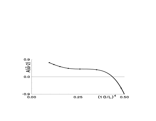
Figure 3: The deviation of the extrapolated effective exponent $\Delta\widetilde{\omega}(L)=\widetilde{\omega}(L)-2$ as a function of $L^{-4}$. The extrapolation has been made by using the calculated $G(r)$ values in Tab. 2 up to the size $L+2$. A linear convergence to zero would be expected in absence of any correction term with exponent $\omega<2$.

We have illustrated this systematic and smooth deviation in Fig. 3. The only reasonable explanation of this behavior is that the expansion (21) necessarily contains the exponent $2$ and, likely, also the exponent $4$, and at the same time it contains also a correction of a very small amplitude with $\omega<2$. The latter explains the increase of $\Delta\widetilde{\omega}(L)$. Namely, the correction to scaling for $L^{1/4}G(L)$ behaves like $const\cdot L^{-2}\left[1+\mathcal{O}\left(L^{-2}\right)+\varepsilon\,L^{2-\omega}\right]$ with $\varepsilon\ll 1$, which implies a slow crossover of the effective exponent $\omega_{eff}(L)$ from the values about $2$ to the asymptotic value $\omega$. Besides, in the region where $\varepsilon\,L^{2-\omega}\ll 1$ holds, the effective exponent behaves like

$$\omega_{eff}(L)\simeq 2+b_{1}L^{2-\omega}+b_{2}L^{-2}\;,$$ (26)

where $b_{1}\ll 1$ and $b_{2}$ are constants. By using the extrapolation of $\omega_{eff}$ with $\omega^{\prime}=2$ in (24) and (25), we have compensated the effect of the correction term $b_{2}L^{-2}$. Besides, by matching the amplitude $b$ in (25) we have compensated also the next trivial correction term $\sim L^{-3}$ in the expansion of $\omega_{eff}(L)$. It means that the extrapolated exponent $\widetilde{\omega}(L)$ does not contain these expansion terms, i. e., we have

$$\widetilde{\omega}(L)=2+b_{1}L^{2-\omega}+\delta\widetilde{\omega}(L)\;,$$ (27)

where $\delta\widetilde{\omega}(L)$ represents a remainder term. It includes the trivial corrections like $L^{-4}$, $L^{-5}$, etc., and also subleading nontrivial corrections, as well as corrections of order $\left(\varepsilon\,L^{2-\omega}\right)^{2}$, $\left(\varepsilon\,L^{2-\omega}\right)^{3}$, etc., neglected in (26). According to the latter, Eq. (27) is meaningless in the thermodynamic limit $L\to\infty$, but it can be used to evaluate the correction–to–scaling exponent $\omega$ from the transient behavior at large, but not too large values of $L$ where $b_{1}L^{2-\omega}\ll 1$ holds. In our example the latter condition is well satisfied, indeed.

Based on (27), we have estimated the nontrivial correction–to–scaling exponent $\omega$ by using the data of $\widetilde{\omega}(L)$ in Tab 2. We have used two different ansatzs

$$2-\omega_{1}(L)=\ln\left[\Delta\widetilde{\omega}(L)/\Delta\widetilde{\omega}(L-1)\right]/\ln[L/(L-1)]$$ (28)

and

$$2-\omega_{2}(L)=L\,\left[\Delta\widetilde{\omega}(L)-\Delta\widetilde{\omega}(L-1)\right]/\Delta\widetilde{\omega}(L)\;,$$ (29)

as well as the linear combination of them

$$\omega(L)=(1-\alpha)\;\omega_{1}(L)+\alpha\;\omega_{2}(L)$$ (30)

containing a free parameter $\alpha$. We have $\omega(L)=\omega_{1}(L)$ at $\alpha=0$ and $\omega(L)=\omega_{2}(L)$ at $\alpha=1$. In general, the effective exponent $\omega(L)$ converges to the same result $\omega$ at arbitrary value of $\alpha$, but at some values the convergence is better. The results for $2-\omega(L)$ vs $L^{\omega-6}$ at different $\alpha$ values are represented in Fig. 4 by a set of curves. In this scale the convergence to the asymptotic value would be linear (within the actual region where $L\gg 1$ and $b_{1}\,L^{2-\omega}\ll 1$ hold) for $\alpha=0$ at the condition $\delta\widetilde{\omega}(L)\propto L^{-4}$.

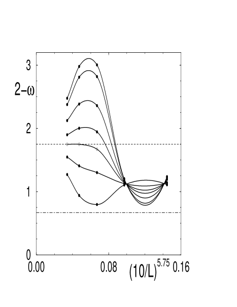
Figure 4: The exponent $2-\omega$ estimated from (30) at different system sizes. From top to bottom (if looking on the left hand side): $\alpha=0,1,3.5,5.75,7.243,9.25,12$. The results at the optimal $\alpha$ value $7.243$ are shown by empty circles. The dashed line indicates our theoretical asymptotic value $2-\omega=1.75$, whereas the dot–dashed line – that proposed in [27].

We have choosen the scale of $L^{-5.75}$, as it is consistent with our theoretical prediction in Sec. 2 that $\omega=1/4$. Nothing is changed essentially if we use slightly different scale as, e. g., $L^{-14/3}$ consistent with the correction–to–scaling exponent $\omega=4/3$ proposed in [27]. As we see from Fig. 4, all curves tend to merge at our asymptotic value $2-\omega=1.75$ shown by a dashed line. The optimal value of $\alpha$ is defined by the condition that the last two estimates $\omega(17)$ and $\omega(18)$ agree with each other. It occurs at $\alpha=7.243$, and the last two points lie just on our theoretical line. A discussion and comparison of our results with those in published literature (e. g., [28]) can be found in [29].

4.4 Comparison to the known exact results and estimation of numerical errors

We have carefully checked our algorithms comparing the results with those obtained via a straightforward counting of all spin configurations for small lattices, as well as comparing the obtained values of the partition function to those calculated from the known exact analytical expressions. Namely, an exact expression for the partition function of a finite–size 2D lattice on a torus with arbitrary coupling constants between each pair of neighbouring spins has been reported in [30] obtained by the loop counting method and represented by determinants of certain transfer matrices. In the standard 2D Ising model with only one common coupling constant $\beta$ these matrices can be diagonalized easily, using the standard techniques [31]. Besides, the loop counting method can be trivially extended to the cases with antiperiodic or mixed boundary conditions discussed in Sec. 3.3. It is necessary only to mention that each loop gets an additional factor $-1$ when it winds round the torus with antiperiodic boundary conditions. We consider the partition functions $Z_{pp}\equiv Z$, $Z_{aa}$, $Z_{ap}$, $Z_{pa}$. In this notation the first index refers to the horizontal or $x$ axis, and the second one – to the vertical or $y$ axis of a lattice illustrated in Fig. 1a; $p$ means periodic and $a$ – antiperiodic boundary conditions. As explained above, the standard methods leads to the following exact expressions:

$$Z_{pp} = \left(Q_{1}+Q_{2}+Q_{3}-Q_{0}\right)/\,2$$

$$Z_{ap} = \left(Q_{0}+Q_{1}+Q_{3}-Q_{2}\right)/\,2$$

$$Z_{pa} = \left(Q_{0}+Q_{1}+Q_{2}-Q_{3}\right)/\,2$$ (31)

$$Z_{aa} = \left(Q_{0}+Q_{2}+Q_{3}-Q_{1}\right)/\,2$$

where $Q_{0}$ is the partition function represented by the sum of the closed loops on the lattice, as consistent with the loop counting method in [31], whereas $Q_{1}$, $Q_{2}$, and $Q_{3}$ are modified sums with additional factors $\exp(\Delta x\cdot i\pi/N+\Delta y\cdot i\pi/L)$, $\exp(\Delta x\cdot i\pi/N)$, and $\exp(\Delta y\cdot i\pi/L)$, respectively, related to each change of coordinate $x$ by $\Delta x=\pm 1$, or coordinate $y$ by $\Delta y=\pm 1$ when making a loop. The standard manipulations [31] yield

$$Q_{i}=2^{NL}\prod\limits_{q_{x},\,q_{y}}\left[\cosh^{2}(2\beta)-\sinh(2\beta)\right.$$ (32)

$$\left.\times\left(\cos\left[q_{x}+\left(\delta_{i,1}+\delta_{i,2}\right)\frac{\pi}{N}\right]+\cos\left[q_{y}+\left(\delta_{i,1}+\delta_{i,3}\right)\frac{\pi}{L}\right]\right)\right]^{1/2}\;,$$

where the wave vectors $q_{x}=(2\pi/N)\cdot n$ and $q_{y}=(2\pi/L)\cdot\ell$ run over all the values corresponding to $n=0,1,2,\ldots,N-1$ and $\ell=0,1,2,\ldots,L-1$. Eq. (32) represents an analytic extension from small $\beta$ region [30]. The correct sign of square roots is defined by this condition, and all $Q_{i}$ are positive except for $Q_{0}$, which vanishes at $\beta=\beta_{c}$ and becomes negative at $\beta>\beta_{c}$. In the case of the periodic boundary conditions, each loop of $Q_{0}$ has the sign $(-1)^{m+ab+a+b}$ [30], where $m$ is the number of intersections, $a$ is the number of windings around the torus in $x$ direction, and $b$ – in $y$ direction. The correct result for $Z_{pp}$ is obtained if each of the loops has the sign $(-1)^{m}$. In all other cases, similar relations are found easily, taking into account the above defined additional factors. Eqs. (31) are then obtained by finding such a linear combination of quantities $Q_{i}$ which ensures the correct weight for each kind of loops.

All our tests provided a perfect agreement between the obtained values of the Greens functions $G(r)$ (a comparison between straightforward calculations and our algorithms), as well as between partition functions for different boundary conditions (a comparison between our algorithms and Eq. (31)). The relative discrepancies were extremely small (e. g., $10^{-15}$), obviously, due to the purely numerical inaccuracy.

We have used the double–precision FORTRAN programs. The numerical errors in Tab. 2 have been estimated by repeating some calculations with twice larger number of digits (REAL*16 option). Thus, the errors in the $G(L)$ values for $L=10$ to $L=17$ are $4.7\cdot 10^{-17}$, $4.06\cdot 10^{-16}$, $-3.52\cdot 10^{-16}$, $-5.65\cdot 10^{-16}$, $1.03\cdot 10^{-15}$, $1.41\cdot 10^{-15}$, $-1.71\cdot 10^{-16}$, and $3.09\cdot 10^{-16}$. To eliminate the summation error for the largest lattice $L=20$, we have split the summation over the configurations of the first row in several parts in such a way that a relatively small part, including only the first 10 000 configurations from the total number of 52 487 nonequivalent ones, gives the main contribution to $Z$ and $Z^{\prime}$. The same trick with splitting in two approximately equal parts has been used at $L=19$. As a result, the numerical errors at $L=18,19,20$ are not much larger than the above listed values for $10\leq L\leq 17$. Hence, the resulting numerical errors in Fig. 4 do not much exceed $0.03$ in the middle part around $2-\omega\sim 1.75$. In Fig. 3, the errors are practically not seen.

5 Generation of pseudo–random numbers

We have found that some of simulated quantities like specific heat of 3D Ising model near criticality are rather sensitive to the quality of pseudo–random numbers. The linear congruatial generators providing the sequence

$$I_{n+1}=(aI_{n}+c)\mathrm{mod}\,m$$ (33)

of integer numbers $I_{n}$ is a convenient choice. We have used in previous section the generator of [33] with $a=843314861$, $c=453816693$, and $m=2^{31}$. The G05CAF generator of NAG library with $a=13^{13}$, $c=0$, and $m=2^{59}$ (generating odd integers) has been extensively used in [35]. We have compared the results of both generators for 3D Ising model, simulated by the Wolff’s cluster algorithm [36], and have found a disagreement by almost $1.8\%$ in the maximal value of $C_{V}$ at the system size $L=48$. Application of the standard shuffling scheme ([38] p. 391) with the length of the shuffling box (string) $N=128$ appears to be not helpful to remove the discrepancy. The problem is that the standard shuffling scheme, where the numbers created by the original generator are put in the shuffling box and picked up from it with random delays in about $N$ steps, effectively removes the short–range correlations between the pseudo–random numbers, but nevertheless it does not essentially change the block–averages $\langle I_{n}\rangle_{k}=k^{-1}\sum_{j=n}^{n+k-1}I_{j}$ over $k$ subsequent steps if $k\gg N$. It means that such a shuffling is unable to modify the low–frequency tail of the Fourier spectrum of the sequence $I_{n}$ to make it more consistent with white noise (an ideal case). The numbers $I_{n}$ repeat cyclically and the block–averages over the cycle do not fluctuate at all in contradiction with truly random behavior. To solve the problem, we have made a second shuffling as follows. We have split the whole cycle of length $m$ of the actual generator with $m=2^{31}$ in $2^{20}$ segments each consisting of 2048 numbers. Starting with 0, we have recorded the beginning numbers of each segment. It allows to restart the generator from the beginning of any segment. The last pseudo–random number generated by our shuffling scheme is used to choose the next number from the shuffling box, exactly as in the standard scheme. In addition, we have used the last but one number to choose at random a new segment after each 2048 steps. This double–shuffling scheme mimics the true fluctuations of the block–averages even at $k\gg m$ and has an extremely long (comparable with $\left(2^{9}\atop 2^{20}\right)\left(2^{20}\right)!$ steps at $N=2^{20}$) cycle. We have used a very large shuffling box with $N=2^{20}$ to make the shuffling more effective. As a consequence, we have reached a perfect agreement with the results of G05CAF generator, which has a rather long cycle even without shuffling.

A hidden problem is the existence of certain long–range correlations in the sequence $I_{n}$ of the original generator of [33]. Namely, pseudo–random numbers of a subset, composed by picking up each $2^{k}$–th element of the original sequence, appear to be rather strongly correlated for $k\geq 20$. It is observed explicitely by plotting such a subsequence $I^{*}_{n}$ vs $n$, particularly, if the first element is choosen $I^{*}_{1}=0$. These correlations reduce the effectiveness of our second shuffling. Correlations of this kind, although well masked, exist also in the sequence of G05CAF generator. Namely, if we choose $I^{*}_{1}=1$ and $k=25$ and generate the coordinates ($x,y$) by means of this subset, then we observe that the $x-y$ plane is filled by the generated points in a non–random way. The origin of these correlations, obviously, is the choice of modulo parameter $m$ as a power of $2$. It, evidently, is the reason for systematical errors in some applications with Swendsen–Wang algorithm discussed in [37]. A promising alternative, therefore, is to use the well known Lewis generator [38], where $m=2^{31}-1$ is a prime number, $a=7^{5}$, and $c=0$, as the original generator of our double–shuffling scheme. (This generator has been tested in [39] and, even without any shuffling, it gave good results for the energy and specific heat of 2D Ising model on $16\times 16$ lattice simulated by Wolff’s cluster algorithm.) As before, the cycle is split in $2^{20}$ segments. However, the first segment now starts with 1. Besides, the first and the last segments contain only 2047 elements instead of 2048. After all numbers of the previous segment are exhausted, a new segment is choosen as follows: if the last but one random number of our shuffling scheme is $I$, then we choose the $k$–th segment, where $k=1+\left[I/2048\right]$. Since we never have $I=0$ or $I=m$, it ensures that each segment is choosen with the probability proportional to its length. We have used the shuffling box of length $N=10^{6}$ for this scheme.

From the theoretical point of view, the latter scheme could provide the best pseudo–random numbers. The test simulations we made in 2D Ising model showed that G05CAF generator, as well as both shuffling schemes provide very accurate results, which indicates that the actually discussed long–range correlations do not have a remarkable effect in our application. We have simulated by the Wolff’s algorithm the mean energy $\langle\varepsilon\rangle$, specific heat $C_{V}$, as well as its derivatives $C^{\prime}_{V}=\partial C_{V}/\partial\beta$ and $C^{\prime\prime}_{V}=\partial^{2}C_{V}/\partial\beta^{2}$ for 2D Ising model at the critical point and have compared the results with those extracted from exact formulae (31) and (32). The test simulations consisting of $4.8\cdot 10^{8}$ and $2.4\cdot 10^{7}$ cluster–algorithm steps have been made for the lattice sizes $L=48$ and $L=256$, respectively. The whole simulation has been split in 24 blocks to estimate the statistical averages and standard errors ($\sigma$) from the last 20 blocks. The simulation with the generator of [33] has revealed systematical errors of about $10\sigma$ for the specific heat and its derivatives at $L=48$. The values provided by the G05CAF generator and our two shuffling schemes agreed with the exact ones within the errors about one $\sigma$. The most serious deviation of $2.37\sigma$ has been observed for $C^{\prime\prime}_{V}$ in the case of $L=48$ simulated by our first shuffling scheme. At $L=48$, one standard deviation $\sigma$ corresponded to $\sim 0.0009\%$ relative error for $\langle\varepsilon\rangle$, $\sim 0.02\%$ error for $C_{V}$, $\sim 0.2\%$ error for $C^{\prime}_{V}$, and $\sim 0.35\%$ error for $C^{\prime\prime}_{V}$. At $L=256$ these errors were $\sim 0.0012\%$, $\sim 0.12\%$, $\sim 3\%$, and $\sim 4\%$, respectively. Furthermore we have used the latter three generators in simulations of 3D Ising model and verification of the simulated values by performing some of the simulations twice with different generators.

6 Test estimations of the critical exponent $\beta$ in 2D Ising model

Based on the well known exact magnetization data $M=\left(1-[\sinh 2K]^{-4}\right)^{\beta}$ of 2D Ising model, we have tested the known method of effective exponents [40, 41] extensively used in our paper. Here $\beta=1/8$ is the magnetization exponent and $K$ is the coupling constant, denoted in this way exceptionally in Secs. 6 to 8.

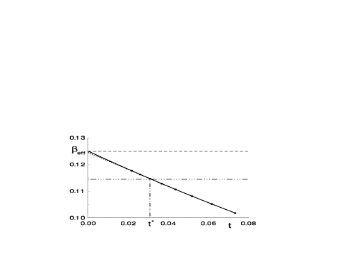
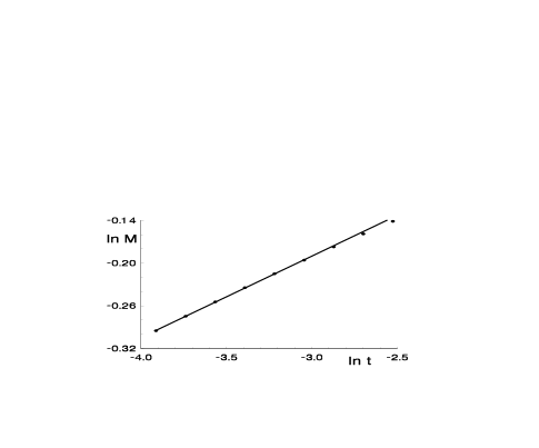
Figure 5: A test estimation of the critical exponent $\beta$ in 2D Ising model by the method of effective exponents (left) and by measuring the slope of the $\ln M$ vs $\ln t$ plot (right). The tiny–dashed and the solid lines in the left–hand–side picture show the linear and the quadratic extrapolations yielding $\beta\simeq 0.1244$ and $\beta\simeq 0.12496$, respectively. The horizontal dashed line shows the exact value $1/8$. The slope of the linear $6$–point fit within $t\in[t_{min};t_{max}]$ in the right–hand–side picture gives $\beta\simeq 0.1144\simeq\beta_{eff}(t^{*})$, where the values $0.1144$ and $t^{*}=\sqrt{t_{min}t_{max}}$ are indicated in the other picture by dot–dot–dashed lines.

The effective critical exponent $\beta_{eff}(t)=\ln[M(at)/M(t/a)]/(2\ln a)$ with $a=2^{1/4}$, calculated from the magnetization data $M(t)$ within the range of the reduced temperatures $t=(K/K_{c})-1\in[0.02;0.08]$ (where $K_{c}$ is the critical coupling) is shown in Fig. 5 (left) by solid circles. Omitting two largest $t$ values, the linear least–squares approximation of $\beta_{eff}(t)$ (tiny dashed line) gives $\beta\simeq 0.1244$, and the quadratic fit of all points (solid line) yields $\beta\simeq 0.12496$ in close agreement with the exact value $0.125$. For comparison, the most popular method of estimation of critical exponents by simply measuring the slope of a log–log plot, as illustrated in the right–hand–side picture (Fig. 5), yields a relatively poor result $\beta\simeq 0.1144$ in spite of the fact that the actually used piece of the log–log plot (6 smallest $t$ values) looks very linear. Up to now we have discussed the exact data only. In the case of Monte Carlo data with the statistical errors, say, about the symbol size, we would be unable to detect the very small deviations from linearity and could easily get a very good, but nevertheless misleading linear fit. In other words, such a simple measuring of critical exponent is unreliable since there is clearly a danger to get an uncontrolled systematical error. Such a measurement within $t\in[t_{min};t_{max}]$ practically yields the mean slope of the log–log plot within this interval, which is nothing but an effective exponent. It corresponds just to one point on the $\beta_{eff}(t)$ plot, i. e., to $\beta_{eff}(t^{*})$ at $t^{*}=\sqrt{t_{min}t_{max}}$, as indicated in Fig. 5 (left) by dot–dot–dashed lines. The method of effective exponents has been designed to control the systematical errors of such simple measurements and eliminate them by a suitable extrapolation. Inclusion of corrections to scaling directly in the ansatz for row data (in this case $M$) is another way to eliminate the systematical errors. However, we greatly prefer the method of effective exponents since it can be well controlled visually. This method is also sensitive enough to distinguish between a power–like and a logarithmic singularity of specific heat, as discussed in Sec. 9.

There are no essential problems reported in literature, as regards the MC estimation of the critical exponent $\beta$ in 2D Ising model. It is because the simulations can be done easily much closer to the critical point than in our test example. However, the problem remains in 3D case. The systematical errors in the measured $\beta$ values are caused by the corrections to scaling, so that $t^{\theta}$ rather than $t$ is an essential parameter. For the smallest reduced temperatures $t\geq 0.0005$ considered in the published literature [42] we have $t^{\theta}>0.022$ with the RG value of the correction–to–scaling exponent $\theta\simeq 0.5$, and $t^{\theta}>0.079$ with our (GFD) value $\theta=1/3$. It means that the systematical errors of the simple (naive) measurements of $\beta$ can be even larger than in our 2D test example with $t^{\theta}\equiv t\geq 0.02$.

7 Estimation of the critical coupling of 3D Ising model

Here we discuss the critical coupling $K_{c}$ of 3D Ising model, which is relevant to our estimations of the critical exponent $\beta$ in Sec. 8. The most accurate MC values reported in literature are $K_{c}=0.22165459(10)$ [43], $K_{c}\simeq 0.2216545$ [44], and $K_{c}=0.2216544(3)$ [42]. One of the recent estimates of HT series expansion is $K_{c}=0.221654(1)$ [45]. We have estimated the critical coupling from our MC results for the pseudocritical couplings $\tilde{K}_{c}(L)$ which correspond to $U=1.6$, where $U=\langle M^{4}\rangle/\langle M^{2}\rangle^{2}$. Note that $1-U/3$ is the Binder cumulant which may have the values from $0$ (at high temperatures) to $2/3$ (at low temperatures). In the thermodynamic limit $L\to\infty$ it changes jump–likely at $K=K_{c}$, so that $\lim\limits_{L\to\infty}\tilde{K}_{c}(L)=K_{c}$ holds for any given $U$ within $1<U<3$.

The values $\tilde{K}_{c}(48)=0.22164540(118)$, $\tilde{K}_{c}(64)=0.22165095(153)$, $\tilde{K}_{c}(96)=0.221653069(734)$, $\tilde{K}_{c}(128)=0.221653945(453)$, $\tilde{K}_{c}(192)=0.221654550(316)$, $\tilde{K}_{c}(256)=0.221654755(163)$, and $\tilde{K}_{c}(384)=0.221654532(109)$ have been obtained by an iterative method similar to that described in Sec. 9.

The data suggest that the pseudocritical coupling has a maximum at $L\sim 256$. Since $dU/dK$ is negative, such a qualitative behavior is expected in view of the known results [14], according to which the universal value of $U$ at $K=K_{c}$ and $L\to\infty$ is slightly larger than $1.6$ and, therefore, $\tilde{K}_{c}(L)$ should approach $K_{c}$ from above. According to the finite–size scaling theory, $\tilde{K}_{c}(L)-K_{c}\propto L^{-1/\nu}\left[1+\mathcal{O}\left(L^{-\omega}\right)\right]$ holds at large $L$, where $\omega=\theta/\nu$. We have found that the data within a wide range of sizes can be well described by the Pade approximation rather than by a simple ansatz with the correction–to–scaling term. Namely, the formula

$$\tilde{K}_{c}(L)\simeq K_{c}+\mathcal{L}^{-1/\nu}\;\frac{a_{0}+a_{1}\mathcal{L}^{-\omega}}{1+\mathcal{L}^{-\omega}}\;,$$ (34)

where $\mathcal{L}=L/L_{0}$ and $L_{0}$ corresponds to the maximum of $\tilde{K}_{c}(L)$ plot, well fits the data within the whole range of sizes $L\in[48;384]$. The location of the maximum is the only characteristic length measure for the $\tilde{K}_{c}(L)$ plot, which should transform to the correct asymptotic form somewhat beyond this maximum. It motivates our specific choice of $L_{0}$, which otherwise is not well defined as a fitting parameter. Fortunately, the results remain practically unchanged if we take, say, twice smaller or twice larger value of $L_{0}$.

Assuming our (GFD) exponents $\nu=2/3$ and $\omega=0.5$ (correction–to–scaling exponent for the magnetization), a fitting of all data points to (34) yields $K_{c}=0.22165407(29)$ with the goodness of fit [46] $Q=0.897$. To eliminate the systematical errors, we have discarded the two smallest sizes, which yields $K_{c}=0.22165386(51)$ with $Q=0.797$. It agrees within the error bars with the value $0.2216544(3)$ of [42] and the value $0.221654(1)$ of [45]. Our value is provided by the fit within $L\in[96;384]$ at $L_{0}=234$. It is shifted up (down) only by $5.5\cdot 10^{-8}$ ($6.1\cdot 10^{-8}$) at a twice smaller (larger) $L_{0}$. It is also not very sensitive to the choice of the exponents $\nu$ and $\omega$. Assuming the RG exponents $\nu=0.63$ and $\omega=0.8$, we obtain $K_{c}=0.22165395(46)$ with $Q=0.795$. Further we have used both our values of $K_{c}$ and those reported in literature in various estimations of the critical exponent $\beta$.

8 Estimation of the critical exponent $\beta$ from the magnetization data in 3D Ising model

Based on the well known scaling relation $2\beta=d\nu-\gamma$, we find from (2) and (3), where $j=0$ and $m=3$ holds at $n=1$, the GFD value $\beta=3/8$ of the magnetization exponent $\beta$ for 3D Ising model. This value is remarkably larger than the usually believed ones about $0.326$ [12]. We suppose that the asymptotic exponent $\beta$ not only for the Ising model, but also for the Heisenberg model is larger than provided by approximate RG theories and known numerical estimates. In polycrystalline Ni ($n=3$), the increase of the effective exponent $\beta_{eff}$ well above the RG value 0.3662 [47] has been established experimentally in [48], where the authors have found the asymptotic estimate $\beta=0.390(3)$. This value clearly disagree within error bars with the RG prediction, but agree with our value $11/28=0.3928\ldots$ predicted for the $n=3$ case ($m=3$, $j=2$). Also the critical exponent $\gamma$ measured in most of experiments on Ni and Fe ranges from 1.28 to 1.35 (see [48, 49, 50] and references therein), and only some experimentators have obtained a larger value about 1.41 – the only value cited in [12]. One of the best experimental methods is to use the Kouvel–Fisher plot, since $T_{c}$ and $\gamma$ are determined simultaneously with no fitting parameters [49]. This method yields the value $\gamma=1.35$ [49, 51] which is believed among (some) experimentators to be the asymptotic exponent (see the references in [49]). Our prediction $\gamma=19/14\simeq 1.357$ is remarkably consistent with this value.

Let us now return to the Ising model. The spontaneous magnetization $M$ of 3D Ising model has been considered in [52, 53, 54, 42]. An empirical formula

$$M(\hat{t})=\hat{t}^{0.32694109}\left(1.6919045-0.34357731\,\hat{t}^{0.50842026}-0.42572366\,\hat{t}\right)$$ (35)

with $\hat{t}=1-0.2216544/K$ has been found in [42] which fits the simulated at three linear sizes $L=64,128,256$ of the lattice and extrapolated to the thermodynamic limit data of $\langle\mid M\mid\rangle$ within the range of the reduced temperatures $\hat{t}\simeq t=(K/K_{c})-1>0.0005$. We have made an approximate estimatiom of the spontaneos magnetization $M(t)$ in the thermodynamic limit from our simulated values of $\langle\mid M\mid\rangle$ at $L=200$ to compare the results with (35). Besides, we have made accurate MC simulations by the Wolff’s algorithm [36] at $t\geq 0.000086$ for system sizes up to $L=410$ to verify the critical exponent $\beta\simeq 0.3269$ proposed by (35).

We have performed the simulations at certain values of coupling constants $K_{i}$,

$$K_{i}=K_{c}^{*}+\frac{0.224-K_{c}^{*}}{(\sqrt{2})^{i}}\;,\hskip 12.91663pt-2\leq i\leq 14$$ (36)

(rounded to 9 digits after the decimal point), where $K_{c}^{*}=0.2216545$ is the critical coupling estimated in [44]. We have choosen $K_{0}=0.224$ to compare our results with those reported in [53, 54]. Each next $K_{i}$ value is $\sqrt{2}$ times closer to $K_{c}^{*}$ than the previous one.

Our MC simulations have been split typically in $51$ blocks (bins) to calculate the average value an standard deviation $\sigma$ from the last $50$ bins. As a test, we have checked that a splitting in twice larger blocks provides consistent values of $\sigma$, i. e., the blocks were large enough to justify our treatment of the block–averages as statistically independent quantities. In most of the cases one bin included $J=120000$ cluster updates, which corresponds to $J\langle M^{2}\rangle$ complete updates of the whole system or sweeps, as consistent with the known improved cluster estimator $\langle M^{2}\rangle=L^{-d}\langle c\rangle$ [38], where $\langle c\rangle$ is the average cluster size. Somewhat shorter simulations have been performed for our estimations of $\langle\mid M\mid\rangle$ in Tab. 3. The results at our smallest $K$ value $K_{14}=0.221672824$ have been obtained by an averaging over four runs, i. e., $4\times 50\times 60000$ cluster updates. Note that the auto–correlation time of the Wolff’s algorithm at criticality is only few (2 or 3) sweeps [36]. The MC measurements were made frequently with respect to this auto–correlation time, i. e., the fraction of moved spins between the measurements was about $0.15$ or smaller. In all cases we have discarded no less than $300$ sweeps from the beginning of the simulation. We have verified that the system has been equilibrated well enough by comparing the estimates from separate smaller parts of the whole simulation.

Our $\langle\mid M\mid\rangle$ data for $K_{-2}\leq K\leq K_{3}$ are listed in Tab. 3. The second shuffling scheme described in Sec. 5 has been used as a source of pseudo–random numbers for this simulation.

Table 3: The simulated values of $\langle\mid M\mid\rangle$ at four different system sizes $L$ in the range of coupling constants $K_{3}\leq K\leq K_{-2}$.

	$L=60$	$L=80$	$L=120$	$L=200$
$K=K_{-2}$	0.460754(205)	0.460695(149)	0.460787(155)	0.460493(96)
$K=K_{-1}$	0.414874(203)	0.414845(236)	0.414329(162)	0.414503(141)
$K=K_{0}$	0.372813(339)	0.372785(240)	0.372939(212)	0.372389(142)
$K=K_{1}$	0.334641(378)	0.334207(221)	0.334246(211)	0.334327(122)
$K=K_{2}$	0.299917(295)	0.299268(298)	0.299473(211)	0.299621(163)
$K=K_{3}$	0.268433(402)	0.268930(294)	0.268807(286)	0.268723(200)

The values of $\langle\mid M\mid\rangle$ are only slightly varied with $L$, and those at the largest two sizes $L=120$ and $L=200$ agree or almost agree within the error bars. According to [54], the latter size more than 22 times exceeds the correlation length $\xi$ at $K\geq K_{3}$, which is quite enough to estimate the thermodynamic limit. Our data at $L=200$ are in a reasonable agreement with the corresponding values 0.460435, 0.414490, 0.372471, 0.334258, 0.299652, and 0.268412 given by (35) at $K=K_{-2}$ to $K=K_{3}$. Our result at $K=K_{0}=0.224$, i. e. $M=0.372389(142)$ or $M^{2}=0.138674(106)$, agree within the error bars with the $M^{2}$ value $0.138708(39)$ reported in [53], as well as with $M^{2}$ value $0.1387488(75)$ obtained in [54].

Our estimation of the critical exponent $\beta$ is based on the analysis of the effective exponent

$$\beta_{eff}(t)=\frac{\ln\langle M^{2}(t_{1},L(t_{1}))\rangle-\ln\langle M^{2}(t_{2},L(t_{2}))\rangle}{2(\ln t_{1}-\ln t_{2})}\;,$$ (37)

where $\ln t=(\ln t_{1}+\ln t_{2})/2$, $L(t)t^{\nu}=const$, and $\langle M^{2}(t,L)\rangle$ is the statistically averaged squared magnetization at the given $t$ and $L$. The effective exponent is the average slope of the $0.5\ln\langle M^{2}\rangle$ vs $\ln t$ plot within $t\in[t_{1};t_{2}]$, calculated at a fixed scaling argument $Lt^{\nu}$ which corresponds to a certain asymptotic value of $L/\xi$ at $t\to 0$, where $\xi\sim t^{-\nu}$ is the correlation length. For any given ratio $t_{2}/t_{1}$, the values of $\beta_{eff}(t)$ lie on a smooth analytical curve converging to the true asymptotic exponent $\beta$ at $t\to 0$. Besides, the estimates obtained at slightly different values of $t_{2}/t_{1}$ well coincide with each other. We have choosen $L(t)=256(\tilde{t}/t)^{\nu}$, where $\tilde{t}$ is a reference value of the reduced temperature at $K=K_{12}=0.221691148$. In this case $L(t)$ approximately corresponds to the minimum of $\langle\mid M\mid\rangle$ vs $L$ plot [55], and the deviations from the thermodynamic limit are small. Two slightly different values for the correlation length exponent $\nu$ have been used, i. e., $\nu=2/3$ (our value) and $\nu=0.63$ (RG value).

We have made the simulations at $L$ values close to $L(t)$, which allow us to estimate $\langle M^{2}(t,L(t))\rangle$ both at $\nu=2/3$ and $\nu=0.63$ by a linear interpolation of $\langle M^{2}\rangle$ vs $L^{-d}$ plot. This plot is linear at $L\to\infty$, as discussed in [52]. At $K=K_{13},K_{14}$, all (three) points have been fit together to get a more reliable result. The simulated values are listed in Tab. 4.

Table 4: Squared magnetization $\langle M^{2}(K,L)\rangle$ at different coupling constants $K$ and system sizes $L$. The simulated values have been obtained by using G05CAF pseudo–random number generator, except those marked by an asterisk, for which our second shuffling scheme (Sec. 5) has been applied. The value of [55] is marked by a dagger.

L	$\langle M^{2}(K_{-1},L)\rangle$	L	$\langle M^{2}(K_{0},L)\rangle$	L	$\langle M^{2}(K_{1},L)\rangle$
12	0.186509(149)	16	0.148333(120)	20	0.119325(134)
13	0.182897(143)	18	0.144657(144)	21	0.117712(98)
14	0.180291(156)	19	0.143549(125)	23	0.116133(116)
15	0.177886(154)			24	0.115459(127)
L	$\langle M^{2}(K_{2},L)\rangle$	L	$\langle M^{2}(K_{3},L)\rangle$	L	$\langle M^{2}(K_{4},L)\rangle$
25	0.095551(72)	32	0.076381(92)	40	0.060932(105)
26	0.095077(113)	32	$0.076290(109)^{*}$	41	0.060583(87)
28	0.093522(99)	35	0.074865(99)	44	0.059919(68)
29	0.092933(107)	36	0.074543(103)	45	0.059726(92)
L	$\langle M^{2}(K_{5},L)\rangle$	L	$\langle M^{2}(K_{6},L)\rangle$	L	$\langle M^{2}(K_{7},L)\rangle$
50	0.048762(79)	64	0.038874(80)	80	0.031042(79)
51	0.048476(89)	64	$0.038872(69)^{*}$	83	0.030865(68)
55	0.047911(79)	69	0.038338(83)	86	0.030618(69)
56	0.047747(75)	70	0.038252(79)
L	$\langle M^{2}(K_{8},L)\rangle$	L	$\langle M^{2}(K_{9},L)\rangle$	L	$\langle M^{2}(K_{10},L)\rangle$
101	0.024673(66)	128	0.019726(73)	161	0.015670(49)
104	0.024538(60)	128	$0.019735(50)^{*}$	166	0.015575(46)
107	0.024466(63)	133	0.019596(59)
L	$\langle M^{2}(K_{11},L)\rangle$	L	$\langle M^{2}(K_{12},L)\rangle$	L	$\langle M^{2}(K_{13},L)\rangle$
203	0.012498(45)	256	0.009936(47)	315	0.007950(32)
206	0.012464(62)	256	$0.009862(49)^{\dagger}$	320	0.007911(43)
		256	$0.009976(87)^{*}$	320	$0.007943(39)^{*}$
				325	0.007901(38)
L	$\langle M^{2}(K_{14},L)\rangle$	L	$\langle M^{2}(K_{14},L)\rangle$	L	$\langle M^{2}(K_{14},L)\rangle$
390	0.006344(25)	400	0.006317(27)	410	0.006275(25)

In most of the cases the G05CAF pseudo–random number generator has been used, whereas some of the values, which are marked by an asterisk, have been simulated by our second shuffling scheme (Sec. 5). The first value at $K=K_{12}$ and $L=256$ has been obtained from $50\times 90000$ cluster updates. The second one represents the result of [55] extracted from the simulation of approximately the same length with the same G05CAF generator. As we see, different simulations confirm each other within the error bars. We have made a weighted averaging (with the weights proportional to the simulation length which is roughly $\propto 1/\sigma^{2}$) of the overlaping simulation results to obtain statistically more reliable values for our further analysis.

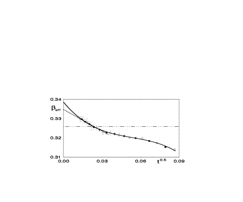
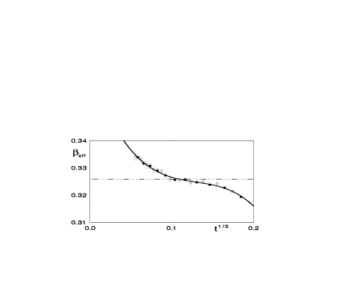
Figure 6: The effective critical exponent $\beta_{eff}$ vs $t^{\theta}$ with $\theta=0.5$ (left) and $\theta=1/3$ (right). The values calculated from (37) with $\nu=0.63$, $K_{c}=0.22165395$ (left) and $\nu=2/3$, $K_{c}=0.22165386$ (right) are shown by solid circles (averaged over $K=K_{i+j},K_{i+5-j}$ with $j=0,1,2$) and empty circles (averaged over $K=K_{i+j},K_{i+4-j}$ with $j=0,1$). Solid lines represent the cubic fits, whereas the dashed line (left) shows the linear $12$–point fit. The dot–dot–dashed line shows the RG prediction $\beta\simeq 0.3258$ [47].

We have calculated from (37) and plotted in Fig. 6 the effective critical exponent $\beta_{eff}$ as a function of $t^{\theta}$ with the RG exponents $\nu=0.63$ and $\theta=0.5$ (left), as well as with the exponents of GFD theory $\nu=2/3$ and $\theta=1/3$ (right). The corresponding self consistent estimates of the critical coupling $K_{c}=0.22165395(46)$ and $K_{c}=0.22165386(51)$ have been used, obtained in Sec. 7 from the Binder cumulant data within $L\in[96;384]$. The results of a weighted averaging over the estimates obtained at $K=K_{i+j},K_{i+5-j}$ with $j=0,1,2$ are shown by solid circles, whereas the values averaged over $K=K_{i+j},K_{i+4-j}$ with $j=0,1$ are depicted by empty circles. The $\beta_{eff}$ values at $K=K_{j},K_{j+\ell}$ have been taken with the weights $\propto\ell^{2}$, which approximately minimize the resulting statistical errors, taking into accont that the individual errors are roughly proportional to $1/\ell$.

In both cases (left and right) the plot of the effective exponent has an inflection point and is well described by a cubic curve, although the last 12 points (smallest $t$ values) can be well fit by a straight line, too. The linear dashed–line fit with the RG exponents (left) yields $\beta=0.3347(24)$ at a fixed $K_{c}=0.22165395$. Taking into account the uncertainty in $K_{c}$, we have $\beta=0.3347(52)$. This value reduces to $0.3302(37)$ if we take $K_{c}=0.2216544(3)$ estimated in [42]. Nevertheless, in both cases it is slightly larger than the RG value $0.3258$ [47] (dot–dashed line), supported by the high temperature (HT) series expansion [45], and also a bit larger than the value of [42] $\beta=0.3269(6)$ [ansatz (35)]. The linear fit, in fact, takes into account the leading correction to scaling only. The cubic fit at $K_{c}=0.22165395(46)$ (solid curve), which includes also two sub–leading corrections, tends to deviate up to $\beta=0.3385(73)$ ($0.3385(37)$ at a fixed $K_{c}$) in a worse agreement with the RG prediction. Assuming the critical coupling $K_{c}=0.2216544(3)$ of [42], the cubic fit gives $\beta=0.3324(52)$. It is worthy to mention that the fits supporting the RG value with a striking accuracy can be produced easily without simulations so close to the critical point. For instance, omitting the 5 smallest $K$ values (10 points on the $\beta_{eff}$ plot), which roughly corresponds to the simulation range $t>0.0005$, the linear $10$–point fit yields $\beta=0.3262(16)$ at $K_{c}=0.2216544(3)$ (the $K_{c}$ value of [42]) and $\beta=0.3259(15)$ at $K_{c}=0.22165459(10)$ (the $K_{c}$ value of [43]).

Taking into account that the $\beta_{eff}$ data are correlated, the statistical errors of the extrapolated values have been estimated as $\left(\sum_{i}\delta_{i}^{2}\right)^{1/2}$, where $\delta_{i}$ is the partial error due to the uncertainty in the $i$–th value of $\langle M^{2}\rangle$.

A self consistent extrapolation within the GFD theory is illustrated in the right hand side picture (Fig. 6). The cubic fit gives $\beta=0.366(16)$ in agreement with the expected exact result $0.375$. Unfortunately, there is still a very large extrapolation gap, so that we cannot make too serious conclusions herefrom. It is necessary to go even much closer to the critical point in this case with simultaneous reduction of the error in the estimated $K_{c}$ value.

9 Estimation of the singularity of specific heat in 3D Ising model from the finite–size scaling of MC data

It is commonly believed [47] that the specific heat $C_{V}$ of 3D Ising model on an infinitely large lattice has a power–like singularity, i. e., $C_{V}\sim t^{-\alpha}$ at $t\to 0$. According to the finite–size scaling theory, it would mean that

$$C_{V}\sim t^{-\alpha}f\left(L^{1/\nu}t\right)\equiv L^{\alpha/\nu}\tilde{f}\left(L^{1/\nu}t\right)$$ (38)

holds at small $t$ in the finite–size scaling region $t\sim L^{-1/\nu}$. Here $\nu$ is the exponent of correlation length, whereas $f(z)$ and $\tilde{f}(z)=z^{-\alpha}f(z)$ are the scaling functions. The maximum of the $C_{V}$ vs $t$ plot is located at a certain value of the scaling argument $z=L^{1/\nu}t$ at $L\to\infty$, which would mean that the maximum values scale as

$$C_{V}^{\mbox{\scriptsize max}}(L)\propto L^{\alpha/\nu}\hskip 12.91663pt\mbox{at}\hskip 8.61108ptL\to\infty\;.$$ (39)

An estimation of the exponent $\alpha/\nu$ from the slope of the log–log plot then gives us the effective exponent $(\alpha/\nu)_{eff}=\partial\ln C_{V}^{\mbox{\scriptsize max}}(L)/\partial\ln L$, which is varied due to the corrections to scaling like

$$(\alpha/\nu)_{eff}\simeq(\alpha/\nu)+const\cdot L^{-\omega}\;,$$ (40)

where $\omega=\theta/\nu$ is the correction–to–scaling exponent. Note that specific heat contains also an analytic background contibution which influences this behaviour. We have found, however, that this influence is very small in the actually considered range of sizes if the constant background term is of order one, as expected from physically–intuitive considerations.

We allow a possibility that the specific heat has a logarithmic singularity, as consistent with [56] and [5]. It means that Eq. (38) is replaced with

$$C_{V}\sim\ln t\cdot f\left(L^{1/\nu}t\right)$$ (41)

and (40) – with

$$(\alpha/\nu)_{eff}\simeq\frac{1}{\ln(L/L_{0})}\;,$$ (42)

where $L_{0}$ is a constant length scale. Although one believes usually that the singularity of $C_{V}$ is power–like with $\alpha\simeq 0.11$, no strong numerical evidences exist which could rule out the logarithmic singularity (41). The problem is that $\ln t$ behaves almost like a weak power of $t$ with the effective exponent $1/\ln t$, e. g., like $t^{-0.11}$ at $t\sim 10^{-4}$. Moreover, below we will show that the finite–size scaling of the maximal values of $C_{V}$ is even very well consistent with (42) in favour of the logarithmic singularity.

We have tested our method in 2D Ising model, where the logarithmic singularity of specific heat is well known. We have considered the effective exponent

$$(\alpha/\nu)_{eff}(L)=\ln\left[C_{V}^{\mbox{\scriptsize max}}(2L)/C_{V}^{\mbox{\scriptsize max}}(L/2)\right]/\ln 4\;,$$ (43)

which is defined by finite differences of the log–log plot. It coincides with$\partial\ln C_{V}^{\mbox{\scriptsize max}}(L)/\partial\ln L$ at large $L$ where the log–log plot is almost linear. Based on exact data, extracted from (31) and (32), we have found that the effective exponent $(\alpha/\nu)_{eff}(L)$ within $L\in[48;512]$ is fairly well described by ansatz (42) with $L_{0}=0.572$ and remarkably worse described by ansatz (40). It is evident from Fig. 7, where $(\alpha/\nu)_{eff}$ vs $x(L)=1/\ln\left(L/L_{0}\right)$ plot (solid circles) well coincides with the theoretical straight line and is much more linear than the $(\alpha/\nu)_{eff}$ vs $x(L)=10L^{-1}$ plot (empty circles). Thus, our method allows to distinguish between the logarithmic singularity and a powerlike singularity including correction to scaling of the kind $\propto L^{-\omega}$, where $\omega=1$ holds in 2D case.

Figure 7: The effective exponent $(\alpha/\nu)_{eff}$ of 2D Ising model depending on $x(L)=1/\ln(L/L_{0})$ with $L_{0}=0.572$ (solid circles) and $x(L)=10L^{-1}$ (empty circles). The solid straight line represents the approximation $(\alpha/\nu)_{eff}=1/\ln(L/L_{0})$.

The specific heat as well as its derivatives with respect to the coupling constant $\beta$ can be calculated easily from the Boltzmann’s statistics. Thus, omitting an irrelevant prefactor, the specific heat is given by

$$C_{V}=N\left(\langle\varepsilon^{2}\rangle-\langle\varepsilon\rangle^{2}\right)\;,$$ (44)

and the derivatives of (44) are

$$\frac{\partial C_{V}}{\partial\beta} = N^{2}\left(3\langle\varepsilon\rangle\langle\varepsilon^{2}\rangle-\langle\varepsilon^{3}\rangle-2\langle\varepsilon\rangle^{3}\right)$$ (45)

$$\frac{\partial^{2}C_{V}}{\partial\beta^{2}} = N^{3}\left(12\langle\varepsilon\rangle^{2}\langle\varepsilon^{2}\rangle-3\langle\varepsilon^{2}\rangle^{2}-4\langle\varepsilon\rangle\langle\varepsilon^{3}\rangle-6\langle\varepsilon\rangle^{4}+\langle\varepsilon^{4}\rangle\right)\;,$$ (46)

where $N=L^{3}$ is the total number of spins and $\varepsilon$ is the energy per spin. The maximum of specific heat is located at a pseudocritical coupling $\tilde{\beta}_{c}$ which is defined by the condition $\partial C_{V}/\partial\beta=0$. It can be found by the Newton’s iterations

$$\tilde{\beta}_{c}^{(n+1)}=\tilde{\beta}_{c}^{(n)}-\frac{\partial C_{V}/\partial\beta}{\partial^{2}C_{V}/\partial\beta^{2}}\;,$$ (47)

where $\tilde{\beta}_{c}^{(m)}$ denotes the $m$–th approximation of $\tilde{\beta}_{c}$, and the derivatives are calculated from (45) and (46) at $\beta=\tilde{\beta}_{c}^{(n)}$.

We have used the Wolff’s algorithm (in 3D case) to estimate these derivatives in each iteration consisting of either $5\cdot 10^{5}$ (at $L\leq 48$) or $10^{6}$ MC steps. Besides, the first iteration has been used only for equilibration of the system retaining the initial estimate of $\tilde{\beta}_{c}$. After few iterations $\beta$ ($C_{V}$) reaches $\tilde{\beta}_{c}$ ($C_{V}^{\mbox{\scriptsize max}}$) within the statistical error and further fluctuates arround this value. In principle, the fluctuation amplitude can be reduced to an arbitrarily small value by increasing the number of MC steps in one iteration.

An obvious advantage of this iterative method is that the maximal value of $C_{V}$ can be evaluated in one simulation without any intermediate analysis. Omitting first $5$ iterations, the mean values and the standard deviations have been evaluated by jakknife method [38] from the rest $19$ iterations, except the largest sizes $64\leq L\leq 128$, where only 4 iterations (with twice larger number of MC steps) have been discarded and 11 iterations have been used for the estimations. In the most of the cases the first shuffling scheme discussed in Sec. 5 has been used as a source of pseudo–random numbers, and the simulated values have been verified by repeating the simulations at $L=24$, 48, and 96 with the G05CAF generator. The perfect agreement confirms our results.

We have averaged the values of $C_{V}^{\mbox{\scriptsize max}}$ over both simulations at $L=24$, 48, and 96 to reduce the statistical errors in the estimated effective critical exponent (43). Our results are summarized in Tab. 5.

Table 5: The MC estimates of the maximal values of the specific heat $C_{V}^{\mbox{\scriptsize max}}$, the pseudocritical couplings $\tilde{\beta}_{c}$, and the effective critical exponents $(\alpha/\nu)_{eff}$ depending on the system size $L$. The marked values have been simulated by G05CAF pseudo–random number generator.

L	$C_{V}^{\mbox{\scriptsize max}}$	$\tilde{\beta}_{c}$	$(\alpha/\nu)_{eff}$
3	16.4445(61)	0.233595(31)
4	21.532(10)	0.234207(26)
6	28.908(27)	0.231090(33)	0.66742(89)
8	34.155(28)	0.228561(23)	0.5552(14)
12	41.481(49)	0.225771(20)	0.4464(12)
16	46.491(85)	0.224436(13)	0.3894(19)
24	53.71(10)	0.223207(13)	0.3333(19)
24	$53.65(10)^{*}$	$0.223193(16)^{*}$
32	58.60(15)	0.2226726(96)	0.3096(20)
48	65.82(25)	0.2222037(97)	0.2784(23)
48	$65.86(18)^{*}$	$0.2221990(87)^{*}$
64	71.41(15)	0.2220053(85)	0.2593(69)
96	78.91(23)	0.2218379(56)
96	$79.01(39)^{*}$	$0.2218387(55)^{*}$
128	83.95(78)	0.2217704(78)

The effective exponent $(\alpha/\nu)_{eff}(L)$ within $L\in[12;64]$ is rather well approximated by (42) with $L_{0}=1.258$, as shown in Fig. 8 by solid circles and linear least–squares fit in the scale of $x(L)=1/\ln(L/L_{0})$.

Figure 8: The effective exponent $(\alpha/\nu)_{eff}$ of 3D Ising model depending on $x(L)=1/\ln(L/1.258)$ (solid circles) and $x(L)=2L^{-0.8}$ (empty circles). The lower solid–line fit represents the approximation $(\alpha/\nu)_{eff}=1/\ln(L/L_{0})$ with $L_{0}=1.258$, whereas the upper one corresponds to $(\alpha/\nu)_{eff}=(\alpha/\nu)+2.044L^{-\omega}$ with the RG exponents $\alpha/\nu=0.173$ and $\omega=0.8$. The dashed line shows the logarithmic approximation in the scale of $2L^{-0.8}$. Statistical errors are within the symbol size. The mean squared deviations from the lower and upper solid–line fits are $1.6\cdot 10^{-5}$ and $8.22\cdot 10^{-5}$, respectively.

This is a remarkable agreement, taking into account that ansatz (42) contains only one adjustable parameter $L_{0}$. We have tested also ansatz (40), where the exponents $\alpha/\nu=0.173$ and $\omega=0.8$ have been taken from the perturbative RG theory [47]. In this case the agreement with the data is worse, i. e., the mean squared deviation is $5.14$ times larger, as shown in Fig. 8 by empty circles and linear least–squares fit in the scale of $x(L)=2L^{-0.8}$. It can be well seen also when comparing the linear fit of circles with the evidently better dashed–line fit. The latter represents the lower straight line in the scale of $2L^{-0.8}$ and shows the expected behavior of empty circles at $L\to\infty$ if (42) is the correct ansatz. Note that the main deviations of the data points from the fitted lines in Fig. 8 are not of statistical character, since the statistical errors are remarkably smaller than the symbol size except only the largest $L$ value, where the error is about the symbol size. Due to this reason we have used simple least–squares approximations, minimizing the sum of not weighted squared deviations. These deviations show just the error of the ansatz used and, thus, indicate that (42) is a better approximation than (40) with fixed exponents $\alpha/\nu=0.173$ and $\omega=0.8$ within the actual range of sizes, at least. Moreover, since $L^{-0.8}$ has reached already a rather small value $0.036$ and, therefore, the second–order correction $\sim L^{-1.6}$ should be very small, the observed deviations can be explained easily assuming (42) rather than (40) with the RG exponents. According to our recent findings (based on unpublished simulation data for $L\leq 192$) the discrepancy with the RG value $\alpha/\nu=0.173$ can be explained by the existence of a negative background contribution $C_{0}=-25(3)$ to $C_{V}$ which, however, seems to be unphysically large in magnitude.

It is quite possible that the true value of $\alpha=2-d\nu$ is remarkably smaller than the RG value $0.11$, as consistent with our recent results for the exponent $1/\nu$. We have estimated $(1/\nu)_{eff}=y_{eff}(L)$ from the derivatives of the Binder cumulant $U^{\prime}(L)=dU(L)/d\beta$ (see Sec. 7) at two system sizes $L/2$ and $2L$. They should scale like $U^{\prime}(L)\sim L^{1/\nu}$ at a pseudocritical coupling corresponding to $U=const$. Our data $U^{\prime}(16)=-175.34(0.17)$, $U^{\prime}(32)=-526.65(0.83)$, $U^{\prime}(48)=-1007.8(2.1)$, $U^{\prime}(64)=-1586.8(3.7)$, $U^{\prime}(96)=-3022.8(8.9)$, $U^{\prime}(128)=-4773.6(16.3)$, $U^{\prime}(192)=-9023.4(48.7)$, $U^{\prime}(256)=-14284(88)$, and $U^{\prime}(384)=-27039(171)$ for $U=1.6$ yield $y_{eff}(32)=1.5889(18)$, $y_{eff}(64)=1.5901(27)$, $y_{eff}(96)=1.5812(41)$, $y_{eff}(128)=1.5851(48)$, and $y_{eff}(192)=1.5805(50)$. In analogy to the plots in Fig. 6, one may expect an accelerated further deviation from the perturbative RG value $\simeq 1.587$.

Thus, in spite of the conventional claims that the specific heat of 3D Ising model has a certain power–like critical singularity, accurately predicted by the perturbative RG theory, the actual very accurate MC data for $C_{V}^{\mbox{\scriptsize max}}$ show that it is even more plausible that the singularity is logarithmic.

10 Remarks about other numerical results

There exists a large number of numerical results in the published literature not discussed here and in [5]. A detailed review of these results is given in [57]. The cited there papers report results which disagree with the values of the critical exponents we have proposed in [5].

Particularly, the values of the perturbative RG theory are well confirmed by the HT series expansions [45, 58]. However, we are somewhat sceptical about such a support of one perturbative method by another. It could well happen that the true reason for the agreement is the extrapolative nature of both methods, according to which both methods describe a transient behavior of the system far away from the true critical region. Really, our simulations of the magnetization data within $t\geq 0.0005$ well confirm the RG value of the critical exponent $\beta$, whereas the agreement becomes worse at $t<0.0005$, where the plot of the effective exponent shows a remarkable inflection thus indicating that the true critical region, where the critical exponents can be accurately measured, is $t\ll 0.0005$. This region, of course, cannot be directly accessed by the HT series expansions. Another problem is that the HT estimation of the critical exponent $\alpha$ [58] is based on a priori assumption that the singularity of specific heat is power–like, whereas the MC data (Sec. 9) suggest that it, very likely, is logarithmic.

According to the finite–size scaling theory, $tL^{1/\nu}$ is a relevant scaling argument, so that not too small values of the reduced temperature $t$ are related to not too large system sizes $L\sim t^{-\nu}$. Thus, according to the idea proposed above, it is quite possible that the MC results for finite systems, like also the simulations at finite $t$ values, appear to be in a good agreement with the conventional RG exponents which are valid within a certain range of $t$ and $L$ values well accessible in MC simulations. The huge number of numerical evidences in the published literature (see [57]) for the exponents of the perturbative RG theory certainly is a serious argument. Nevertheless, there is a reason to worry about the validity of these exponents at $t\to 0$ and/or $L\to\infty$ because of the following problems.

• We have made accurate MC simulations of the magnetization (Sec. 8) for unusually large system syzes ($L\leq 410$) much closer to the critical point ($t\geq 0.000086$ instead of $t\geq 0.0005$) than in the published literature, and have found that the agreement with the RG exponent $\beta$ becomes worse in this case.

• Our MC estimation of the exponent $1/\nu$, discussed at the end of Sec. 9, shows a good agreement with the RG value $1.587$ at not too large system sizes. However, the agreement becomes worse when larger than $L=128$ sizes are included.

• A remarkable deviation of the correction–to–scaling exponent $\omega$ from the perturbative RG value $\omega\simeq 0.8$ has been already reported in literature [59], where also larger than usually system sizes $L\leq 256$ (instead of the conventional $L\leq 128$ [35]) have been simulated in application to the Monte Carlo renormalization group techniques, yielding $\omega\simeq 0.7$.

• The confirmation of RG exponents by MC simulations is not unambiguous. There exist also examples where the simulation results are in a remarkable disagreement with these exponents even within the conventionally considered range of sizes and reduced temperatures. A particular example is the finite–size scaling of the maximal values of the specific heat considered in Sec. 9. We are afraid that there are also other such examples, but they are routinely ascribed as unbelievable and do not appear in the published literature.

• It is indeed easy to produce evidences supporting the RG exponents, as we have shown in Sec. 8, just because these exponents describe the behavior of a system not too close to criticality, in the range which can be easily accessed in MC simulations. The problem is that the usual MC measurements yield only effective exponents, as shown in Sec. 6, which exhibit quite large variations also in 3D case, as it is particularly well seen from our plots of the effective exponents. The leading correction–to–scaling term, included in the fitted ansatz, also does not completely solve the problem: in essence it is the same as to make a linear extrapolation of the effective exponent, but, e. g., the $\beta_{eff}(t)$ plots in Fig. 6 are remarkably nonlinear. Therefore, only such evidences are really serious, which show very precisely how the effective exponents provided by simple estimations converge to certain asymptotic values.

If one consider seriously a possibility that the true values of the critical exponents are those proposed in [5], then a question arises why the published MC estimates tend to deviate greatly from these theoretical values. In our opinion, the main reason is that the published simulations have been made too far away from the true critical region (as regards both $t$ and $L$), where the critical exponents can be precisely measured in a simple way routinely used in MC analysis. The plots of the effective exponents in Fig. 6 provide an evidence for this statement: as we have already mentioned (Sec. 6), simple MC measurements yield just such effective exponents, and they are varied. One has to consider corrections to scaling, and not only the leading one, to get better results. However, all the existing (MC) correction–to–scaling analyses in the published literature rely on the RG correction–to–scaling exponents, therefore the disagreement with the predictions in [5] is not surprising.

Finally, our theory provides a self consistent explanation why much smaller $t$ values and/or much larger system syzes $L$ has to be considered, as compared to the known simulations. It is because the correction–to–scaling exponent $\omega=\theta/\nu=0.5$ in our theory is remarkably smaller than that of the RG theory $\omega\simeq 0.8$, which implies that the decay of corrections to scaling is relatively slow. In fact, the reduced temperatures we have reached in our simulations of the magnetization also are still much too large for an accurate estimation of the critical exponent $\beta$ in the right–hand–side picture in Fig. 6. Nevertheless, we can see that the qualitative behavior, at least, is just such as expected from our theory.

11 Conclusions

Summarizing the present work we conclude the following:

1. Critical exponents and corrections to scaling for different physical quantities have been discussed in framework of our [5] recently developed GFD (grouping of Feynman diagrams) theory (Sec. 2).

2. Calculation of the two–point correlation function of 2D Ising model at the critical point has been made numerically by exact transfer matrix algorithms (Secs. 3 and 4). The results for finite lattices including up to 800 spins have shown the existence of a nontrivial correction to finite–size scaling with a very small amplitude and exponent about $1/4$, as it can be expected from our GFD theory.

3. Accurate Monte Carlo simulations of the magnetization of 3D Ising model have been performed by Wolff’s algorithm in the range of the reduced temperatures $t\geq 0.000086$ and system sizes $L\leq 410$ to evaluate the effective critical exponent $\beta_{eff}(t)$ based on the finite–size scaling. Estimates extracted from the data relatively far away from the critical point, within $t\geq 0.0005$, well confirm the value $\beta\simeq 0.3258$ of the perturbative RG theory [47]. However, the effective exponent tends to increase above this value when approaching $T_{c}$. A self consistent extrapolation does not reveal a contradiction with the prediction $\beta=3/8$ of the GFD theory [5], although there is still a large gap between the simulated and extrapolated values. The convergence of $\beta_{eff}$ to the value of GFD theory $\beta=11/28$ has been observed experimentally in Ni [48], where the asymptotic value $0.390(3)$ has been found.

4. An iterative method has been proposed (Sec. 9) which allows a direct simulation of the maximal values of the specific heat, depending on the system size $L$. The simulated data for 3D Ising model within $6\leq L\leq 128$ apparently show a better agreement with the logarithmic critical singularity of the specific heat predicted in [56] (and consistent with our result $\alpha=0$) than with the specific power–like singularity proposed by the perturbative RG theory [47].

References

- [1] L. Onsager, Phys. Rev. 65 (1944) 117
- [2] D. Sornette, Critical Phenomena in Natural Sciences, Springer, Berlin, 2000
- [3] J. G. Brankov, D. M. Danchev, N. S. Tonchev, Theory of Critical Phenomena in Finite–Size Systems: Scaling and Quantum Effects, World Scientific, Singapore, 2000
- [4] Rodney J. Baxter, Exactly Solved Models in Statistical Mechanics, Academic Press, London, 1989
- [5] J. Kaupužs, Ann. Phys. (Leipzig) 10 (2001) 299
- [6] N. Ito, M. Suzuki, Progress of Theoretical Physics, 77 (1987) 1391
- [7] N. Schultka, E. Manousakis, Phys. Rev. B 52 (1995) 7258
- [8] L. S. Goldner, G. Ahlers, Phys. Rev. B 45 (1992) 13129
- [9] J. Kaupužs, Eur. Phys. J. B 45 (2005) 459
- [10] K. G. Wilson, M. E. Fisher, Phys. Rev. Lett. 28 (1972) 240
- [11] Shang–Keng Ma, Modern Theory of Critical Phenomena, W.A. Benjamin, Inc., New York, 1976
- [12] J. Zinn–Justin, Quantum Field Theory and Critical Phenomena, Clarendon Press, Oxford, 1996
- [13] H. Chamati, Eur. Phys. J. B 24 (2001) 241
- [14] M. Hasenbusch, J. Phys. A 32 (1999) 4851
- [15] D. J. Amit, Field theory, the renormalization group, and critical phenomena, World Scientific, Singapore, 1984
- [16] M. E. Fisher, The theory of critical point singularities, In: Critical Phenomena (Editor M. S. Green), Proceedings of the 51st Summer School, Varena, Italy, pp. 73–98, Acad. Press., London, 1971
- [17] M. J. Stephen, Phys. Lett. 56 A (1976) 149
- [18] J. Kaupužs, Int. J. Mod. Phys. C 16 (2005) 1121
- [19] J. A. Redinz, A. C. N. de Magelhaes, Phys. Rev. B 51 (1995) 2930
- [20] T. Koma, H. Tasaki, Phys. Rev. Lett. 74 (1995) 3916
- [21] J. Fröhlich, T. H. Spencer, Comm. Math. Phys. 81 (1981) 527
- [22] E. Brezin, J. Zinn–Justin, Phys. Rev. B 14 (1976) 3110
- [23] I. D. Lawrie, J. Phys. A 14 (1981) 2489
- [24] H. A. Yang, J. H. H. Perk, Int. J. Mod. Phys. B 16 (2002) 2089
- [25] M. Henkel, Conformal invariance and critical phenomena. Texts and monographs in physics, Springer, Berlin, 1999
- [26] K. Huang, Statistical Mechanics, John Wiley & Sons, New York 1963
- [27] M. Barma, M. Fisher, Phys. Rev. Lett. 53 (1984) 1935
- [28] B. Nickel, J. Phys. A 33 (2000) 1693
- [29] J. Kaupužs, Computational Methods in Applied Mathematics 5 (2005) 72
- [30] A. Bednorz, J. Phys. A 33 (2000) 5457
- [31] L. Landau, E. Lifshitz, Course of Theoretical Physics, Part 5: Statistical Physics, §141, Moscow, 1964
- [32] B. A. Berg, J. Stat. Phys. 82 (1996) 323
- [33] G. E. Forsytne, M. A. Malchom, C. B. Moler, Computer Methods for Mathematical Computations, Englewood Cliffs, N. J.: Prentice–Hall, 1977
- [34] N. A. Alves, J. R. Drugowich, U. H. E. Hansmann, J. Phys. A 33 (2000) 7489
- [35] M. Hasenbusch, Int. J. Mod. Phys. 12 (2001) 911
- [36] U. Wolff, Phys. Rev. Lett. 62 (1989) 361
- [37] G. Ossola, A. D. Sokal, Phys. Rev. E 70 (2004) 027701
- [38] M. E. J. Newman, G. T. Barkema, Monte Carlo Methods in Statistical Physics, Clarendon Press, Oxford, 1999
- [39] A. M. Ferrenberg, D. P. Landau, Y. J. Wong, Phys. Rev. Lett. 69 (1992) 3382
- [40] H. G. Ballesteros, L. A. Fernandez, V. Martin–Mayor, A. M. Sudupe, Phys. Lett. B 387 (1996) 125
- [41] C. Holm, W. Janke, Phys. Rev. B 48 (1993) 936
- [42] A. L. Talapov, H. W. Blöte, J. Phys. A 29 (1996) 5117
- [43] H. W. J. Blöte, L. N. Shchur, A. L. Talapov, Int. J. Mod. Phys. C 10 (1999) 1137
- [44] M. Hasenbusch, K. Pinn, S. Vinti, Phys. Rev. B 59 (1999) 11 471
- [45] P. Butera, M. Comi, Phys. Rev. B 62 (2000) 14837
- [46] W. H. Press, B. P. Flannery, S. A. Teukolsky, W. T. Vetterling, Numerical Recipes – The Art of Scientific Computing, Cambridge University Press, Cambridge, 1989
- [47] R. Guida, J. Zinn–Justin, J. Phys. A 31 (1998) 8103
- [48] N. Stüsser, M. Th. Rekveldt, T. Spruijt, Phys. Rev. B 33 (1986) 6423
- [49] T. Bitoh, T. Shirane, S. Chikazawa, J. Phys. Soc. Jap. 62 (1993) 2837
- [50] T. Shirane, T. Moriya, T. Bitoh, J. Phys. Soc. Jap. 64 (1995) 951
- [51] J. S. Kouvel, M. E. Fisher, Phys. Rev. 136A (1964) 1626
- [52] N. Ito, M. Suzuki, J. Phys. Soc. Jap. 60 (1991) 1978
- [53] N. Ito, In Proc. of Computer-Aided Statistical Physics (Taipei, Taiwan, 1991), AIP Conference Proceedings 248, p. 136
- [54] M. Caselle, M. Hasenbusch, J. Phys. A 30 (1997) 4963
- [55] M. Hasenbusch, private communication
- [56] A. L. Tseskis, Zh. Eksp. Teor. Fiz. 102 (1992) 508
- [57] A. Pelissetto, E. Vicari, Physics Reports 368 (2002) 549
- [58] H. Airisue, T. Fujiwara, Phys. Rev. E 67 (2003) 066109
- [59] R. Gupta, P. Tamayo, Int. J. Mod. Phys. C 7 (1996) 305