Effect of Disorder Strength on Optimal Paths
in Complex Networks

Abstract

We study the transition between the strong and weak disorder regimes in the scaling properties of the average optimal path $\ell_{\rm opt}$ in a disordered Erdős-Rényi (ER) random network and scale-free (SF) network. Each link $i$ is associated with a weight $\tau_{i}\equiv\exp(ar_{i})$, where $r_{i}$ is a random number taken from a uniform distribution between $0$ and $1$ and the parameter $a$ controls the strength of the disorder. We find that for any finite $a$, there is a crossover network size $N^{*}(a)$ at which the transition occurs. For $N\ll N^{*}(a)$ the scaling behavior of $\ell_{\rm opt}$ is in the strong disorder regime, with $\ell_{\rm opt}\sim N^{1/3}$ for ER networks and for SF networks with $\lambda\geq 4$, and $\ell_{\rm opt}\sim N^{(\lambda-3)/(\lambda-1)}$ for SF networks with $3<\lambda<4$. For $N\gg N^{*}(a)$ the scaling behavior is in the weak disorder regime, with $\ell_{\rm opt}\sim\ln N$ for ER networks and SF networks with $\lambda>3$. In order to study the transition we propose a measure which indicates how close or far the disordered network is from the limit of strong disorder. We propose a scaling ansatz for this measure and demonstrate its validity. We proceed to derive the scaling relation between $N^{*}(a)$ and $a$. We find that $N^{*}(a)\sim a^{3}$ for ER networks and for SF networks with $\lambda\geq 4$, and $N^{*}(a)\sim a^{(\lambda-1)/(\lambda-3)}$ for SF networks with $3<\lambda<4$.

I Introduction

The subject of complex networks has been widely explored in the past few years in part due to its broad range of applications to social, biological and communication systems Albert02 ; Barabasi02 ; Buchanan02 ; Watts03 ; Dorogovtsev03 ; Pastor . In a real world network, whether it be a communication network or transport network, the time $\tau_{i}$ taken to traverse a link $i$ may not be the same for all the links. In other words, there is a “cost” or a “weight” $\tau_{i}$ associated with each link, and the larger the weight on a link, the harder it is to traverse this link. In such a case, the network is said to be disordered.

Consider two nodes $A$ and $B$ on such a disordered network. In general, there will be a large number of paths connecting $A$ and $B$. Among these paths, there is usually a single path for which the sum of the costs $\sum\tau_{i}$ along the path is minimum and this path is called the “optimal path.” The problem of optimal paths on networks is of import since the purpose of many real networks is to provide an efficient traffic route between its nodes.

When most of the links on the path contribute to the sum, the system is said to be “weakly disordered” (WD). In some cases, however, the cost of a single link along the path dominates the sum. In this case every path between two nodes can be characterized by a value equal to the maximum cost along that path, and the path with the minimal value of the maximum cost is the optimal path between the two nodes. This limit of disorder is called the strong disorder (SD) limit (“ultrametric” limit) Cieplak and we refer to the optimal path in this limit as the min-max path.

The procedure to implement disorder on a network is as follows Cieplak ; Porto99 ; Brauns01 ; Brauns03 . One assigns to each link $i$ of the network a random number $r_{i}$, uniformly distributed between 0 and 1. The cost associated with link $i$ is then

$$\tau_{i}\equiv\exp(ar_{i}),$$ (1)

where $a$ is the parameter which controls the broadness of the distribution of link costs. The parameter $a$ represents the strength of disorder. The limit $a\rightarrow\infty$ is the strong disorder limit, since for this case only one link dominates the cost of the path.

There are distinct scaling relationships between the length of the average optimal path $\ell_{\rm opt}$ and the network size (number of nodes) $N$ depending on whether the network is strongly or weakly disordered Brauns03 . For strong disorder Brauns03 , $\ell_{\rm opt}\sim N^{\nu_{\rm opt}}$, where $\nu_{\rm opt}=1/3$ for Erdős-Rényi (ER) random networks ER59 and for scale-free (SF) Albert02 networks with $\lambda>4$, where $\lambda$ is the exponent characterizing the power law decay of the degree distribution. For SF networks with $3<\lambda<4$, $\nu_{\rm opt}=(\lambda-3)/(\lambda-1)$. For weakly disordered ER networks and for SF networks with $\lambda>3$, $\ell_{\rm opt}\sim\ln N$. Porto et al. Porto99 considered the optimal path transition from weak to strong disorder for 2-D and 3-D lattices, and found a crossover in the scaling properties of the optimal path that depends on the disorder strength $a$, as well as the lattice size $L$.

Here we show that similar to regular lattices, there exists for any finite $a$, a crossover network size $N^{*}(a)$ such that for $N\ll N^{*}(a)$, the scaling properties of the optimal path are in the strong disorder regime while for $N\gg N^{*}(a)$, the network is in the weak disorder regime. We evaluate the function $N^{*}(a)$. The structure of the paper is as follows. In Section II we derive a scaling approach for the transition from weak disorder to strong disorder of the optimal path. In Section III we present simulation results which support the scaling Ansatz. Finally, in Section IV we conclude with an analytic justification for the scaling of the transition.

Figure 1: Schematic representation of the transition in the topology of the optimal path with system size $N$ for a given disorder strength $a$. The solid line shows the optimal path at a finite value of $a$ connecting two nodes indicated by the filled circles. The portion of the min-max path that is distinct from the optimal path is indicated by the dashed line. (a) For $N\ll N^{*}(a)$ (i.e. $\ell_{\infty}\ll\ell^{*}(a)$), the optimal path coincides with the min-max path, and we expect the statistics of the SD limit. (b) For $N=N^{*}(a)$ (i.e. $\ell_{\infty}=\ell^{*}(a)$), the optimal path starts deviating from the min-max path. (c) For $N\gg N^{*}(a)$ (i.e. $\ell_{\infty}\gg\ell^{*}(a)$), the optimal path has almost no links in common with the min-max path, and we expect the statistics of the WD limit.

II Scaling Approach

In general, the average optimal path length $\ell_{opt}(a)$ in a disordered network depends on $a$ as well as on $N$. In the following we use instead of $N$ the min-max path length $\ell_{\infty}$ which is related to $N$ as $\ell_{\infty}\equiv\ell_{\rm opt}(\infty)\sim N^{\nu_{\rm opt}}$ and hence $N$ can be expressed as a function of $\ell_{\infty}$,

$$N\sim\ell_{\infty}^{1/\nu_{\rm opt}}.$$ (2)

Thus, for finite $a$, $\ell_{\rm opt}(a)$ depends on both $a$ and $\ell_{\infty}$. We expect that there exists a crossover length $\ell^{*}(a)$, corresponding to the crossover network size $N^{*}(a)$, such that (i) for $\ell_{\infty}\ll\ell^{*}(a)$, the scaling properties of $\ell_{\rm opt}(a)$ are those of the strong disorder regime, and (ii) for $\ell_{\infty}\gg\ell^{*}(a)$, the scaling properties of $\ell_{\rm opt}(a)$ are those of the weak disorder regime. In Fig. 1, we show a schematic representation of the change of the optimal path as the network size increases.

In order to study the transition from strong to weak disorder, we introduce a measure which indicates how close or far the disordered network is from the limit of strong disorder. A natural measure is the ratio

$$W(a)\equiv\frac{\ell_{\rm opt}(a)}{\ell_{\infty}}.$$ (3)

Using the scaling relationships between $\ell_{\rm opt}(a)$ and $N$ in both regimes, and $\ell_{\infty}\sim N^{\nu_{\rm opt}}$ (see Section I), we get

$$\ell_{\rm opt}(a)\sim\begin{cases}\ell_{\infty}\sim N^{\nu_{\rm opt}}&\text{[SD]}\cr\ln\ell_{\infty}\sim\ln N&\text{[WD].}\end{cases}$$ (4)

From Eq. (3) and Eq. (4) it follows,

$$W(a)\sim\begin{cases}{\rm const.}&\text{[SD]}\cr\ln\ell_{\infty}/\ell_{\infty}&\text{[WD].}\end{cases}$$ (5)

We propose the following scaling Ansatz for $W(a)$,

$$W(a)=F\left({\ell_{\infty}\over\ell^{*}(a)}\right),$$ (6)

where

$$F(u)\sim\begin{cases}{\rm const}.&\text{$u\ll 1$}\cr\ln(u)/u&\text{$u\gg 1$,}\end{cases}$$ (7)

with

$$u\equiv{\ell_{\infty}\over\ell^{*}(a)}.$$ (8)

The dependence of $\ell^{*}(a)$ on $a$ can be estimated as follows. In the strong disorder limit, the costs on the links for any path on the network typically differ by at least an order of magnitude. This means that for a min-max path of $\ell$ links (or length $\ell$), if we arrange the costs of the links in descending order, then two consecutive costs typically differ at least by an order of magnitude. If $r_{1}$ and $r_{2}$ are the random numbers associated with two such consecutive links, with $r_{1}>r_{2}$, then the ratio of the costs on the links is

$${\tau_{1}\over\tau_{2}}=\exp(a\Delta r),$$ (9)

where $\Delta r\equiv r_{1}-r_{2}$. Thus, in the case of strong disorder we must have $a\Delta r\gg 1$. Consequently the transition to weak disorder occurs when all the links become equivalent in order of magnitude, i.e., when $a\Delta r\sim 1$. The value of $\Delta r$ depends on the length of the path. If the distribution of random numbers on the min-max path is uniform, then $\Delta r\sim 1/\ell$ for a min-max path of length $\ell$. The condition for the transition, $a\Delta r\sim 1$ is satisfied at the crossover length $\ell^{*}(a)$ which implies that

$$\ell^{*}(a)\sim a.$$ (10)

Therefore, from Eq. (6), $W(a)$ must be a function of $\ell_{\infty}/a$.

III Simulation Results

Next we describe the details of our numerical simulations and show that the results agree with our theoretical predictions. To construct an ER network of size $N$ with average node degree $\langle k\rangle$, we start with $\langle k\rangle N/2$ edges and randomly pick a pair of nodes from the total possible $N(N-1)/2$ pairs to connect with each edge. The only condition we impose is that there cannot be multiple edges between two nodes.

In order to generate SF networks, we use the Molloy-Reed algorithm Molloy . Each node is assigned a random integer $k$ taken from a power-law distribution

$$P(k)=\left({k\over k_{0}}\right)^{-\lambda},$$ (11)

where $k_{0}$ is the minimal possible number of links that a node possesses. Next, we randomly select a node and attempt to connect each of its $k$ links with randomly selected $k$ nodes that still have free positions for links. The disorder in the link costs is then implemented using the procedure described in Brauns01 .

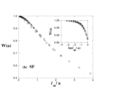
Figure 2: Test of Eqs. (6) and (7). (a) $W(a)$ plotted as a function of $\ell_{\infty}/a$ for different values of $a$ for ER networks with $\langle k\rangle=4$. The different symbols represent different $a$ values: $a=8$($\circ$), $a=16$($\Box$), $a=22$($\diamond$), $a=32$($\bigtriangleup$), $a=45$($+$), and $a=64$($\ast$). (b) Same for SF networks with $\lambda=3.5$. The symbols correspond to the same values of disorder as in (a). The insets show $W(a)$ plotted against $\log(l_{\infty}/a)$, and indicate for $\ell_{\infty}\ll a$, $W(a)$ approaches a constant in agreement with Eq. (7).

To obtain $\ell_{\infty}$, we use the algorithm proposed by Cieplak et al. Cieplak , modified as described in Ref. Brauns203 . With this modification we reach system sizes of $N=2^{16}=65~{}536$. In order to obtain the optimal path for a given realization, we use the Dijkstra algorithm Porto99 . We calculate the average optimal path $\ell_{\rm opt}(a)$ by taking the average of the optimal paths over $10^{6}$ pairs of nodes.

In Fig. 2 we show the ratio $W(a)$ for different values of $a$ plotted against $\ell_{\infty}/\ell^{*}(a)\equiv\ell_{\infty}/a$ for ER networks with $\langle k\rangle=4$ and for SF networks with $\lambda=3.5$. The excellent data collapse is consistent with the scaling relations Eq. (6). Fig. 3 shows the scaled quantities $W(a)u=\ell_{\rm opt}(a)/\ell^{*}(a)$ vs. $\ln u\equiv\ln(\ell_{\infty}/\ell^{*}(a))\equiv\ln(\ell_{\infty}/a)$, for both ER networks with $\langle k\rangle=4$ and for SF networks with $\lambda=3.5$. The curves are linear at large $u\equiv\ell_{\infty}/\ell^{*}(a)$, supporting the validity of the logarithmic term in Eq. (7) for large $u$.

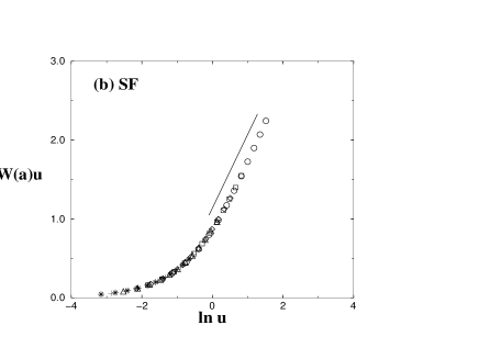
Figure 3: (a) Plot of $W(a)u=\ell_{\rm opt}(a)/\ell^{*}(a)=\ell_{\rm opt}(a)/a$ vs $\ln u\equiv\ln(\ell_{\infty}/\ell^{*}(a))=\ln(\ell_{\infty}/a)$ for ER networks with $\langle k\rangle=4$ for different values of $a$. (b) Plot of $W(a)u=\ell_{\rm opt}(a)/\ell^{*}(a)=\ell_{\rm opt}(a)/a$ vs $\ln u=\ln(\ell_{\infty}/\ell^{*}(a))=\ln(\ell_{\infty}/a)$ for SF networks with $\lambda=3.5$. The values of $a$ represented by the symbols in (a) and (b) are the same as in Fig. (2).

IV Discussion

We next develop analytic arguments that support Eq. (10). These arguments will lead to a clearer picture about the nature of the transition of the optimal path with disorder strength.

We begin by making few observations about the min-max path. In Fig. 4 we plot the average value of the random numbers $r_{n}$ on the min-max path as a function of their rank $n$ ($1\leq n\leq\ell_{\infty}$) for ER networks with $\langle k\rangle=4$ and for SF networks with $\lambda=3.5$. This can be done for a min-max path of any length but in order to get good statistics we use the most probable min-max path length. We call links with $r\leq p_{c}$ “black” links, and links with $r>p_{c}$ “gray” links, following the terminology of Ioselevich and Lyubshin Ios04 where $p_{c}$ is the percolation threshold of the network Cohen00 .

Figure 4: Dependence on rank $n$ of the average values of the random numbers $r_{n}$ along the most probable optimal path for (a) ER random networks of two different sizes $N=4096$ ($\Box$) and $N=16384$ ($\circ$) and, (b) SF random networks.

We make the following observations regarding the min-max path:

• For $r_{n}<p_{c}$, the values of $r_{n}$ decrease linearly with rank $n$, implying that the values of $r$ for black links are uniformly distributed between $0$ and $p_{c}$, consistent with the results of Ref. Szabo03 . This is shown in Fig. 4.

• The average number of black links, $\langle\ell_{b}\rangle$, along the min-max path increases linearly with the average path length $\ell_{\infty}$. This is shown in Fig. 5a.

• The average number of gray links $\langle\ell_{g}\rangle$ along the min-max path increases logarithmically with the average path length $\ell_{\infty}$ or, equivalently, with the network size $N$. This is shown in Fig. 5b.

The simulation results presented in Fig. 5 pertain to ER networks; however, we have confirmed that the observations (ii) and (iii) also hold for SF networks.

Figure 5: (a) The average number of links $\langle\ell_{b}\rangle$ with random number values $r\leq p_{c}$ on the min-max path plotted as a function of its length $\ell_{\infty}$ for an ER network, showing that $\langle\ell_{b}\rangle$ grows linearly with $\ell_{\infty}$. (b) The average number of links $\langle\ell_{g}\rangle$ with random number values $r>p_{c}$ on the min-max path versus $\ln N$ for an ER network, showing that $\langle\ell_{g}\rangle\sim\ln N$. The inset shows the successive slopes, indicating that in the asymptotic limit $\langle\ell_{g}\rangle\approx 1.55\ln N$.

Next we will discuss our observations using the concept of the optimal spanning tree. The optimal spanning tree (OST) is a subset of links of a connected graph which provides an optimal path from node $A$ (which serves as the root of the tree) to any other node on the graph. When the total weight of this path is dominated by the largest weight of the links along the path (strong disorder limit), the OST does not depend on the root and is determined only by the structure of the original graph and a particular realization of the disorder. In this limit, the OST becomes identical to the minimal spanning tree (MST) Szabo03 ; Dob . The path on the MST between any two nodes $A$ and $B$, is the optimal path between the nodes in the strong disorder limit—i.e, the min-max path.

To construct the MST, we remove links in the descending order of their costs $\tau_{i}$. If removal of a link destroys the connectivity of the graph, we restore that link. This procedure is continued till there are exactly $N-1$ links remaining. At this point the number of remaining black links is

$$N_{b}={N\langle k\rangle p_{c}\over 2},$$ (12)

where $\langle k\rangle$ is the average degree of the original graph and $p_{c}$ is given by Cohen00

$$p_{c}={\langle k\rangle\over\langle k^{2}-k\rangle}.$$ (13)

The black links give rise to $N_{c}$ disconnected clusters. One of these is a spanning cluster, called the giant component. The $N_{c}$ clusters are linked together into a connected tree by exactly $N_{c}-1$ gray links (see Fig. 6). Each of the $N_{c}$ clusters is itself a tree, since a random graph can be regarded as an infinite dimensional system, and at the percolation threshold in an infinite dimensional system the clusters can be regarded as trees. Thus the $N_{c}$ clusters containing $N_{b}$ black links, together with $N_{c}-1$ gray links form a spanning tree consisting of $N_{b}+N_{c}-1$ links.

Thus the MST provides a min-max path between any two points on the graph. Since the MST connects $N$ nodes, the number of links on this tree must be equal to $N-1$, so

$$N_{b}+N_{c}=N.$$ (14)

From Eq. (12) and Eq. (14) it follows that

$$N_{c}=N\left(1-{\langle k\rangle p_{c}\over 2}\right).$$ (15)

Therefore $N_{c}$ is proportional to $N$.

The path between any two nodes on the MST consists of $\ell_{b}$ black links. Since the black links are the links that remain after removing all links with $r>p_{c}$, the random number values $r$ on the black links are uniformly distributed between $0$ and $p_{c}$ in agreement with observation (i) and Ref. Szabo03 .

Since there are $N_{c}$ clusters which include clusters of nodes connected by black links as well as isolated nodes, the MST can be described as an effective tree of $N_{c}$ nodes, each representing a cluster, and $N_{c}-1$ gray links. We call this tree the “gray tree” (see Fig. 6). This tree is in fact a scale free tree Tomer04 with degree exponent $\lambda_{g}=2.5$ for ER networks and for scale for networks with $\lambda\geq 4$, and $\lambda_{g}=(2\lambda-3)/(\lambda-2)$ for SF networks with $3<\lambda<4$ exp1 . If we take two nodes $A$ and $B$ on our original network, they will most likely lie on two distinct effective nodes of the gray tree. The number of gray links encountered on the min-max path connecting these two nodes will therefore equal the number of links separating the effective nodes on the gray tree. Hence the average number of gray links $\langle\ell_{g}\rangle$ encountered on the min-max path between an arbitrary pair of nodes on the network is simply the average diameter of the gray tree. Our simulation results (see Fig. 5b) indicate that

$$\langle\ell_{g}\rangle\sim\ln N.$$ (16)

Since $\langle\ell_{g}\rangle\sim\ln\ell_{\infty}\ll\ell_{\infty}$, the average number of black links $\langle\ell_{b}\rangle$ on the min-max path scales as $\ell_{\infty}$ in the limit of large $\ell_{\infty}$ in agreement with observation (2) as shown in Fig. 5a.

Figure 6: Schematic representation of the structure of the minimal spanning tree, at the percolation threshold, with G being the giant component. Inside each cluster, the nodes are connected by black links to form a tree. The dotted lines represent the gray links which connect the finite clusters to form the gray tree. In this example $N_{c}=4$ and the number of gray links equals $N_{c}-1=3$.

Now we will discuss the implications of our findings for the crossover from strong to weak disorder. From observations (i) and (ii), it follows that for the portion of the path belonging to the giant component, the difference between consecutive random values $\Delta r$ is given by $\Delta r=p_{c}/\langle\ell_{b}\rangle$. Hence we can approximate the sum of weights of such links by the sum of the geometric progression

$$\sum^{\ell_{b}}_{k=1}\exp(ka\Delta r)={\exp(a\Delta r)[\exp(ap_{c})-1]\over\exp(a\Delta r)-1}\equiv\exp(ar^{\ast}),$$ (17)

where $r^{\ast}\approx p_{c}+(1/a)\exp(-ap_{c}/\langle\ell_{b}\rangle)$ exp2 . Since $\langle\ell_{b}\rangle\approx\ell_{\infty}$,

$$r^{\ast}\approx p_{c}+{1\over a}\exp\left({-ap_{c}\over\ell_{\infty}}\right).$$ (18)

Thus restoring a short-cut link between two nodes on the optimal path with $p_{c}<r<r^{\ast}$ may drastically reduce the length of the optimal path. When $ap_{c}\gg\ell_{\infty}$ the probability that such a link exists is negligible, but the probability becomes significant for $ap_{c}\approx\ell_{\infty}$. Hence when the min-max path is of length $\ell_{\infty}\approx ap_{c}$ the deviation of the optimal path from the min-max path becomes significant. The length of the min-max path at which the deviation occurs is precisely the crossover length $\ell^{*}(a)$, and therefore $\ell^{\ast}(a)\sim ap_{c}$. Note that in the case of SF networks, as $\lambda\to 3^{+}$, $p_{c}$ approaches zero and consequently $\ell^{*}(a)\to 0$. This suggests that for any finite value of disorder strength $a$, a SF network with $\lambda=3$ is in the weak disorder regime.

In summary, for both ER random networks and SF networks we obtain a scaling function for the crossover from weak disorder characteristics to strong disorder characteristics. We show that the crossover occurs when the min-max path reaches a crossover length $\ell^{*}(a)$ and $\ell^{*}(a)\sim a$. Equivalently, the crossover occurs when the network size $N$ reaches a crossover size $N^{*}(a)$, where $N^{*}(a)\sim a^{3}$ for ER networks and for SF networks with $\lambda\geq 4$ and $N^{*}(a)\sim a^{\frac{\lambda-1}{\lambda-3}}$ for SF networks with $3<\lambda<4$.

Acknowledgments

We thank the Office of Naval Research, the Israel Science Foundation, and the Israeli Center for Complexity Science for financial support, and R. Cohen, E. Lopez, E. Perlsman, G. Paul, T. Tanizawa, and Z. Wu for discussions.

References

- (1) R. Albert and A.-L. Barabási, Rev. Mod. Phys. 74, 47 (2002).
- (2) A.-L. Barabási, Linked: The New Science of Networks (Perseus Publishing, Cambridge MA, 2002).
- (3) M. Buchanan, Nexus: Small Worlds and the Groundbreaking Theory of Networks (W. W. Norton, New York, 2002).
- (4) D. J. Watts, Six Degrees: The Science of a Connected Age (W. W. Norton, New York, 2003).
- (5) S. N. Dorogovtsev and J. F. F. Mendes, Evolution of Networks: From Biological Nets to the Internet and WWW (Oxford University Press, Oxford, 2003).
- (6) R. Pastor-Satorras and A. Vespignani, Structure and Evolution of the Internet: A Statistical Physics Approach (Cambridge University Press, 2004).
- (7) M. Cieplak, A. Maritan, and J. R. Banavar, Phys. Rev. Lett. 72, 2320 (1994); 76, 3754 (1996).
- (8) M. Porto et al., Phys. Rev. E 60, R2448 (1999).
- (9) L. A. Braunstein et al., Phys. Rev. E 65, 056128 (2001).
- (10) L. A. Braunstein et al., Phys. Rev. Lett. 91, 168701 (2003) .
- (11) P. Erdős and A. Rényi, Publicationes Mathematicae 6, 290 (1959).
- (12) M. Molloy and B. Reed, Random Structures and Algorithms 6, 161 (1995); Combin. Probab. Comput. 7, 295 (1998).
- (13) S. V. Buldyrev et al., Physica A 330, 246 (2003).
- (14) L. A. Braunstein et al., to appear in Lecture Notes in Physics: Proceedings of the 23rd CNLS Conference, “Complex Networks,” Santa Fe 2003, edited by E. Ben-Naim, H. Frauenfelder, and Z. Toroczkai (Springer, Berlin, 2004).
- (15) A. S. Ioselevich and D. S. Lyubshin, JETP 79, 286 (2004).
- (16) R. Cohen et al., Phys. Rev. Lett. 85, 4626 (2000).
- (17) G. J. Szabó, M. Alava and J. Kertész, Physica A 330, 31 (2003).
- (18) R. Dobrin and P. M. Duxbury, Phys. Rev. Lett. 86, 5076 (2001).
- (19) T. Kalisky et al., to be submitted.
- (20) This is a consequence of the fact that for the original network the clusters at percolation have sizes distributed as Cohen02 , (with for ER networks and for SF networks with , and for SF networks with ) and each node within this cluster has a non-zero probability of connecting to a node outside the cluster.
- (21) R. Cohen et al., Phys. Rev. E 66, 036113 (2002).
- (22) Using and .