Flow profiling of a surface acoustic wave nanopump

Abstract

The flow profile in a capillary gap and the pumping efficiency of an acoustic micropump employing Surface Acoustic Waves is investigated both experimentally and theoretically. Such ultrasonic surface waves on a piezoelectric substrate strongly couple to a thin liquid layer and generate an internal streaming within the fluid. Such acoustic streaming can be used for controlled agitation during, e.g., microarray hybridization. We use fluorescence correlation spectroscopy and fluorescence microscopy as complementary tools to investigate the resulting flow profile. The velocity was found to depend on the applied power somewhat weaker than linearly and to decrease fast with the distance from the ultrasound generator on the chip.

I INTRODUCTION

For a biological hybridization experiment, typically, single stranded DNA is covalently bound to small probe spots on the surface of a glass slide, forming a so-called micro array. A solution containing fluorescently labelled sample molecules is then spread across this micro array where the molecules are allowed to bind to the respective probe spots. Successful hybridization is usually observed as an increase in the fluorescence intensity on a spot. To have a reference, in co-hybridization experiments a two color coding is used. Usually, such experiments are performed in sealed chambers to prevent the thin liquid film above the slide from evaporation. Given the typical film thickness of less than 100 microns, the system exhibits a very small Reynolds number, and the molecules in the fluid can only move diffusively Kamholz and Yager (2001). Diffusion, however, is a very slow process. Even for small molecules such as Rhodamine the distance travelled in water after $10^{3}$ s is only about 1mm. For relatively large DNA molecules the diffusion driven displacement will be even smaller. On the contrary, the binding reaction of complementary DNA strands is a relatively fast process. Especially in the case when the concentration of probe molecules on a spot is much larger than the one of their counterparts in solution, most of the molecules close to their binding partners at the glass slide will become immobilized after a short time. This can lead to the formation of a depletion zone with a lower concentration close to the solid surface. To reach the equilibrium concentration of bound DNA, molecules have to diffuse through the depletion zone, which becomes the time limiting bottleneck for the hybridization process. Typical hybridization assays are therefore performed over night or even over weekend, and then are stopped at some more or less arbitrary point. Such experiments are also referred to as ”end point” experiments. Apart from the above mentioned non-equilibrium conditions, shorter hybridisation times also lead to a lower fluorescence signal intensities. Quite obviously, this process can be accelerated if the molecules were to be actively transported along the solid surface plane. Due to the low diffusion constant of large DNA strands even a slow movement can speed up the hybridisation considerably. Another aspect is that hybridisation is often conducted with more than one kind of DNA with different fluorescent labels simultaneously. The fluorescence intensities of the different immobilized sample molecules are then evaluated quantitatively to interpret the results. However, when the DNA binding reactions were not in equilibrium at the end of the hybridisation time, the results can be misleading.

As the amount of DNA available for a hybridisation experiment is often very limited one has to reduce the volume as much as possible. Therefore, pump driven flow systems Darnton et al. (2001) usually having large dead volumes are not convenient to induce the molecule transport during the hybridisation process. There are numerous other possibilities to actuate thin fluid films, amongst them for example electrokinetic forces Wu and Keh (2003) Zeng et al. (2001).

In this report, we describe a novel technique to actuate a thin liquid film in a capillary gap. We employ surface acoustic waves (SAW) propagating on the surface of a piezoelectric solid to induce acoustic streaming and mixing within the fluid. To understand the fluid dynamics in such a system, we concentrate on how the acoustic streaming transforms into a velocity field profile within a homogeneous DNA solution in the capillary gap.

A surface acoustic wave (SAW) can be excited by the application of a radio frequency signal (RF) to an interdigital transducer (IDT) on a piezoelectric substrate. The wavelength of the excited SAW is defined by the geometry of the IDT. Typical displacement amplitudes of a SAW are in the nanometer range, depending on the applied RF power. If the SAW supporting surface of the substrate is in contact with a liquid, and if the SAW has any displacement component normal to the surface, ultrasonic SAW power is leaking into the fluid in form of an acoustic wave. Therefore, this so-called leaky SAW (LSAW) is expected to decay exponentially with distance from its source.

The interaction between the SAW and the liquid film leads to an internal, acoustically induced streaming. The reason for this is a net pressure gradient in the direction of the sound propagation in the fluid. Usually, this leads to the generation of a fluidic jet, which can be nicely visualized employing a dye solution and a fluorescence video microscope. The captured images are evaluated in a subsequent image processing step, being a versatile tool for the interpretation of dynamic processes. This method yields real images of the observed sample as a whole, and therefore reduces the problem of a false interpretation of the data. For more precise measurement of the flow field and velocity, we use fluorescence correlation spectroscopy (FCS) Maiti et al. (1997). In this method, the movement of fluorescent particles can be determined in the focal spot of a confocal microscope by evaluating the autocorrelation function of the intensity fluctuations. This represents the rate of particles entering and leaving the small observation volume.

II The experimental setup and microfluidic characteristics

We assembled a special microfluidic arrangement to induce streaming in a narrow capillary gap between a glas slide and a plexiglass block, containing a SAW device.

Figure 1: The measurement setup for the evolution of dye spots consists of a 200 $\mu$m slit between two plexiglas plates (3x3 cm²) kept in the right distance with spacers. Integrated in the lower plate is the SAW chip, being connected to the RF source outside the fluid film. The transducer is located in the middle of the plate. Images were taken with a video microscope from above through the upper plate.

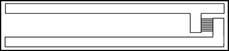
Figure 2: The graph shows the sketch of the 4x23 mm² LiNbO₃ chip with gold structures. Situated on the right side is the interdigitated transducer(1x1 mm²) inducing the SAW perpendicular to the long side of the chip. The contact wires are connected with the Rf power source on the left end.

Fig. 1 gives a sketch of the principal setup as seen from the side. Fig. 2 shows the chip architecture. The width of the gap is controlled by spacers, it can be continuously adjusted down to 30$\mu$m. In the measurements described, we worked with a spacers of 200 $\mu$m. The SAW chip consists of a 128^o rotated Y-cut, X propagating LiNbO₃ single crystal chip.

The IDT consists of 22 finger pairs, 0.85 mm aperture, and a period $\lambda=28\mu$m. The IDT fingers are thermally evaporated 300 nm thick Au electrodes, fabricated by a standard photolithografic technique. The complete chip was protected with a 800 nm thick, sputtered Silicon Dioxide layer, which was removed at the contact pads to allow for electrical connection. The IDT was driven with an AC signal at the resonance frequency $f_{0}$, being defined as $f_{0}=c/\lambda$. For a SAW velocity $c\approx$ 3800 m/s, the frequency $f_{0}$ is hence about 136 MHz. Such an IDT efficiently converts the applied RF signal into an acoustic wave, which in this case is launched as a bidirectional beam perpendicular to the fingers.

If the capillary gap is filled with a fluid, switching on the RF power leads to a flow pattern as sketched in Fig. 3.

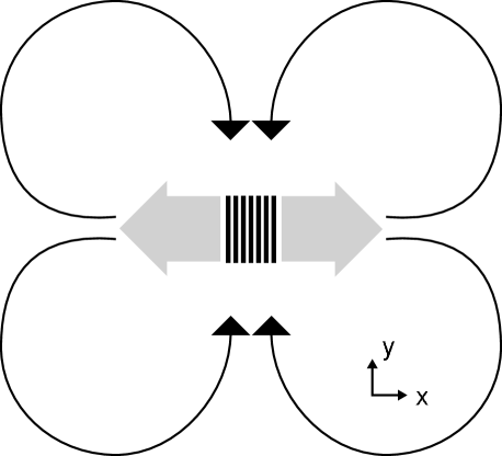
Figure 3: Flow pattern generated by SAW. The fluid is pumped perpendicular to the metal fingers of the IDT and is sucked in parallel to them.

The fluid is expelled from the transducer region to the left and right side and flows back to the IDT from bottom and top. According to the high viscous damping the flow velocity decreases rapidly with distance from the IDT.

Further investigations were focused on the characterization of the flow field. The issue of this work was to find out how the setup can be optimized for agitating a large hybridisation area. For this purpose we first want to discuss the nature of the observed SAW-induced motion.

The propagating LSAW couples to a sound wave in the liquid. Because the sound velocity in fluids $c_{\text{liquid}}$ is always smaller than the LSAW-velocity in the solid substrate, sound is radiated into the liquid under an angle obeying Snellius’ law of diffraction:

$$\sin(\theta_{R})=\frac{c_{\text{liquid}}}{c_{\text{LSAW}}}$$ (1)

This can be understood as a consequence of phase matching between the LSAW and the radiated sound beam in the liquid. This ”mode conversion” leads to an exponential decay of the LSAW. In our case the observed damping in power was about 1dBm per wavelength, which is in good accordance with values found in refs. Shiokawa et al. (1989) and Campbell and Jones (1970). This results in a decrease of 35dBm per mm. In the following we will give a short overview how the sound radiated in the fluid can induce a streaming force.

Sound travelling through a liquid is attenuated by the viscosity along its transmission through the medium. If the intensity is high, this attenuation creates an acoustic pressure gradient along the propagation of the wave. The gradient induces a force in the same direction that causes a flow in the fluid. This conversion of an attenuated sound wave into a steady flow is a nonlinear effect which is known as acoustic streaming. When a SAW, i.e. a surface acoustic wave with a spatially constant amplitude, is in contact with a fluid the acoustic streaming is only a minor effect Shiokawa et al. (1989). Much stronger is the streaming that results from the exponential decay of the LSAW. This decay causes the conversion into sound waves in the liquid within a short distance leading to a large gradient of the sound amplitude and consequently to a strong force that generates the acoustic streaming.

Here we do not want to go into the details of the rather complex mechanism of acoustic streaming Nyborg (1965), Uchida et al. (1995). We only mention that the effective force that causes the steady flow can be expressed in terms of the sound velocity field in the fluid Nyborg (1965):

$${\bf F}=\rho\langle({\bf v}_{f}\cdot\nabla){\bf v}_{f}+{\bf v}_{f}(\nabla\cdot{\bf v}_{f})\rangle$$ (2)

where the angular brackets denote time average that removes the fast oscilations of the sound wave.

Finally we note that the force is proportional to $\omega^{2}$. High force densities therefore can be achieved by means of high LSAW frequencies. On the other hand, lower frequencies lead to smaller damping rates of the LSAW and the force density acts on a larger volume. For an optimal design a trade off has to be found.

III MATERIALS AND METHODS

III.1 Fluorescence Microscopy

Microscope

To visualize the activity of the SAW transducer, a Na-fluorecein solution (1mg/ml) is pipetted into a small hole in the cover of the fluid film. For the excitation of the fluorescence of the dye, blue LEDs are attached to a ring some distance above the cover. Fluorescence images are taken by a video microscope (Olympus, Hamburg) with a suitable filter to suppress the excitation light.

Image processing

Fluorescence images of the evolving Na-fluorescein spot (see Figs. 4, 5 were taken every 10s and stored into an avi movie file. The avi movie was further processed by a procedure converting the pictures into binary images with the help of the Shannon entropy function and detecting the edges of the dye spot with the particle finder algorithm. The coordinates of every edge line were put together in one file (Fig. 6) and the positions of the leading edge to the left and the right was extracted for every recorded point of time. This leads to a distance vs time diagram (Fig. 7) . Differentiating this data yields a speed vs distance diagram. Also, the area of the Na-fluorescein spot and the speed of the area increase can be calculated.

III.2 Fluorescence Correlation Spectroscopy

In 1972 Magde, Elson and Webb published the first work on FCS Magde et al. (1972). In the following years the same authors elaborated the technique and it’s applications in detail Elson and Magde (1974) Magde et al. (1974) Magde et al. (1978), where in the last reference theory and first experiments with FCS on systems with laminar flow are presented. Until the early 1990s FCS was mainly used to determine diffusion properties and kinetic constants of chemical reactions in solution. In 1993 the introduction of a confocal detection optics by Rigler et al. Rigler et al. (1992) gave new impulses to the method. Schwille Schwille et al. (1997), Krichevsky Krichevsky and Bonnet (2002) and Thompson Thompson et al. (2002) have given reviews about the principles, applications and potentials of FCS.

The raw signal in FCS experiments is the time-dependent intensity signal coming from a small and fixed volume ($\approx 0.5\,\mbox{fl}$) created by a laser focus. Fluorescently labelled molecules entering and leaving the open volume lead to fluctuations in the recorded signal $F(t)$:

$$F(t)=q\,Q\,\int_{V}I(\vec{r})C(\vec{r},t)dV$$ (3)

Here, $q$ stands for constant intensity losses due to the experimental setup e.g. detector efficiency, filters. $Q$ is the fluorescence quantum yield of the dye and $C(\vec{r,t})$ denotes the concentration of the labelled particles, $I(\vec{r})=I_{0}\exp(-2(x^{2}+y^{2})/r_{0})\exp(-2z^{2}/z_{0})$ is a combination of the collection efficiency and the excitation profile. If the confocal detection geometry is chosen properly a Gaussian effective volume with radius $r_{0}$ and height $z_{0}$ is a good approximation Hess and Webb (2002).

In this work we want to focus on the possibility to measure flow velocities as it was shown by Gösch et al. Gösch et al. (2000).

The experimental autocorrelation function $g_{2}(t)$ is calculated from the measured fluorescence intensity $F(t)$ by

$$g_{2}(t)=\frac{\langle F(t_{0})F(t_{0}+t)\rangle}{\langle F(t_{0})\rangle^{2}}=1+\frac{\langle\delta F(t_{0})\delta F(t_{0}+t)\rangle}{\langle F(t_{0})\rangle^{2}}.$$ (4)

For Brownian diffusing particles the concentration $C(\vec{r},t)$ is known and can be used to calculate an expected autocorrelation function by combining equation (4) and equation (3)

$$g_{2}(t)=1+\frac{1}{N}\,G_{\mbox{\scriptsize Diff}}(t)$$ (5)

with $N$ denoting the average number of marked objects in the effective focal volume and

$$G_{\mbox{\scriptsize Diff}}(t)=\frac{1}{1+\frac{t}{\tau_{\mbox{\tiny D}}}}\,\frac{1}{\sqrt{1+\frac{t}{f^{2}\tau_{\mbox{\tiny D}}}}}$$ (6)

where $\tau_{\mbox{\scriptsize D}}=\frac{r_{0}^{2}}{4\,D}$ denotes the mean passage time of the particle through the effective volume Eigen and Rigler (1994). and $f=z_{0}/r_{0}$ gives the aspect ratio of the effective volume. With the Rhodamine 6G diffusion constant $D_{\mbox{\scriptsize R6G}}=280\,\mu\mbox{m}^{2}\mbox{s}^{-1}$ Magde et al. (1974) as a reference, the focal waist size and shape parameter were determined ($r_{0}\simeq 0.20\,\mu$m and $f\simeq 8$), and used for all subsequently acquired data.

Equation (6) turns out to be the solution for the ideal case of point-like particles, which is well describing the case where the particle size $R$ is small compared to the focal volume size $r_{0}$. For situations where $R$ is comparable to, or even larger than $r_{0}$ no analytically closed form of equation (6) can be given (particle size effect). The autocorrelation function depends strongly on the distribution of fluorophores on the particle. For spherical particles with radius $R$ an approximate diffusion time can be given Starchev et al. (1998).

$$\tau_{\mbox{\scriptsize D}}=\frac{r_{0}^{2}+R^{2}}{4\,D}$$ (7)

In the presence of a uniform translation in addition to the diffusive particle motion the autocorrelation function becomes

$$g_{2}(t)=1+\frac{1}{N}\,G_{\mbox{\scriptsize Diff}}(t)\,G_{\mbox{\scriptsize Flow}}(t)$$ (8)

where

$$G_{\mbox{\scriptsize Flow}}(t)=\exp(-\frac{t}{\tau_{\mbox{\tiny F}}})$$ (9)

Taking into account the particle size effect the dwell time $\tau_{\mbox{\tiny F}}$ of the particles in the focus is given by

$$\tau_{\mbox{\scriptsize F}}=\frac{r_{0}+R}{v_{\mbox{\tiny Flow}}}$$ (10)

As can be seen from equation (8) the shape and the characteristic decay time of the autocorrelation function is dominated by the faster of the two competing processes. In order to obtain the flow velocities without perturbation by diffusion we used fluorescent microspheres of 1$\mu m$ radius (Fluosperes Yellow-Green 505/515, F-8823, Molecular Probes, Eugene, OR). On the experimentally relevant time-scale the Brownian motion of these spheres is of minor importance. Therefore we could neglect the diffusive term in equation (8).

We used a commercial setup by Carl Zeiss (Jena, Germany) consisting of the module Confocor 2 and the microscope model Axiovert 200 with a Zeiss C-Apochromat 40x NA 1.2 water immersion objective. For excitation, the $514\,$nm line of a $25\,$mW Argon laser was used. Emitted fluorescence was detected at wavelengths longer than $530\,$nm by means of an avalanche photo diode allowing for single-photon counting.

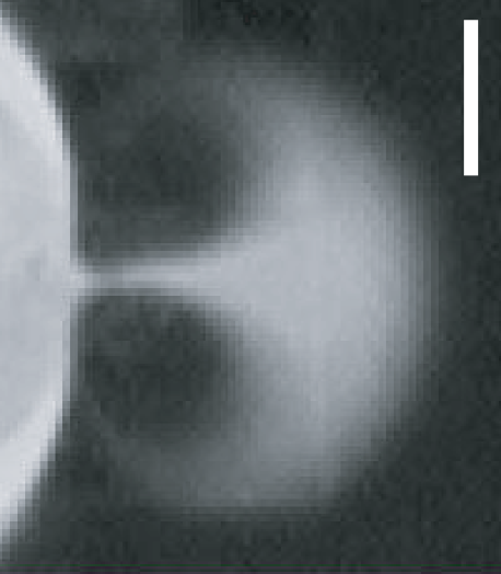
Figure 4: A dye jet pumped by the SAW transducer, shortly after switching the RF-power. In the middle of the transducer the fluid is pumped upwards, on both sides the fluid is sucked in. The bar is 0.5 mm wide.

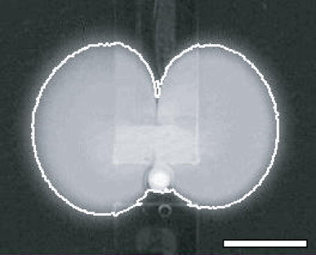
Figure 5: A dye spot after 5 min of SAW pumping (40 mW) is shown. Superimposed is the edge line calculated by the image procedure. The bar is 1mm wide

Figure 6: The edges of a dye spot during the pumping of the SAW transducer (40 mW) are recorded every 10 s and put together in one graph. The evolution from a round spot to a butterfly shape can be observed.

Figure 7: The distance of the dye front as a function of time for 10, 25, 63 and 158 mW RF-power (from bottom to top). The data points where determined every 10 seconds at the line, marked by the arrows in Fig. 6 and connected by lines.

IV RESULTS

As a test for the image processing, a spot of Fluorescein pipetted into the hole of the cover plate was observed for 10 min., with the SAW switched off. The area covered by the dye therefore only increases by diffusion. Using the linear diffusion equation $\langle x^{2}\rangle=2Dt$, a value for the diffusion constant of the dye molecules of D=370$\mu\,\mbox{m}^{2}/\,\mbox{s}$ can be determined which is in good agreement with literature values of 200-400$\mu\,\mbox{m}^{2}/\,\mbox{s}$.

Figure 8: The speed of the growth of the area of the Fluorescein spot is plotted against the particular position of the advancing dye front for 4 different RF-power values (10, 40, 63 and 158 mW from left to right). When the speed reaches the region of the diffusion constant of the dye, the data is superposed by noise. The diffusion constant of Fluorescein (370 $\mu\,\mbox{m}^{2}/\,\mbox{s}$) is marked by a dashed line. For small distances, representing early times, the image processing yields misleading results, since the transducer region is covered by the initial round dye spot.

Figure 9: The distance $x_{D}^{*}$ where the speed of the area growth reaches the diffusion constant of Fluorescein (370 $\mu\,\mbox{m}^{2}/\,\mbox{s}$) dependening on the applied RF-power. Superimposed to the data is a straight line.

Figure 10: The speed of the propagating dye front in the direction of the arrows in Fig. 6 is plotted against the particular position for 4 different RF-power values (10, 40, 63 and 158 mW from left to right). The speed values are calculated by differentiating the front position vs time data. Small distances are not displayed, because the image processing yields misleading results close to the transducer.

Figure 11: The speed of the advancing dye front at a distance 4mm from the SAW transducer is plotted against the RF-power. A straight line has been fitted to the data.

In Fig. 4 a close up image of the area near the transducer is shown, shortly after starting the SAW. The 1mm wide IDT is hidden by the dye solution on the lower side pumping a 200 $\mu$m wide jet to the upper side. The jet becomes broader with increasing distance and a part is transported to the influx areas of the IDT perpendicular to the direction of pumping. After 10 min., the Fluorescein covered area shows a butterfly shape. Employing the image processing the edge of the dye spot is determined every 10 s during the observation time. A border line between the colored and uncolored areas computed this way is plotted in Fig. 5. Collecting the traces of a 10 min. experiment into one graph yields a plot as in Fig. 6. The initial dye spot and the succeeding evolution of the edge lines are visible in this graph. This data was used for determining the evolution speed of the area (Fig. 8). The growth of a Fluorescein spot was observed for 7 different RF-powers and the actual position of the front line in the direction of the arrows in Fig. 6 was recorded. The growth speed decreases fast with distance from the transducer, until the diffusion constant of the dye (370 $\mu\,\mbox{m}^{2}/\,\mbox{s}$) is reached. In the experiment, this position $x_{D}^{*}$ is found to depend linearly on the logarithm of the RF-power, see Fig. 9.

From the movement of the dye front in the symmetry direction marked by the arrows in Fig. 6 the position can be determined as a function of time (Fig. 7). Differentiating this data and plotting it against the x-position of the front leads to a fast decrease of the speed (Fig. 10), similar as found for the growth of the dye covered area. The decay of the velocity with the distance does not change qualitatively upon varying the RF-power. As a quantitative measure we show the velocity at the distance 4mm from the transducer in dependence of the applied RF-power in Fig. 11 . In the measured range a linear dependence yields a reasonable fit although the extrapolation to small powers becomes unphysical.

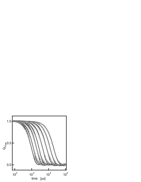
Figure 12: Normalized autocorrelation curves from FCS measurements. The applied power was varied between $150\,\mbox{mW}$ (right) and $500\,\mbox{mW}$ (left) in steps of $50\,\mbox{mW}$. Circles represent the experimental data whereas the lines are fits to equation (9).

Figure 13: Flow velocity as a function of the applied power for three different positions indicated by circles, triangles and squares. The corresponding positions are marked by the same symbols in the Fig.14. Circles represent the results from the fitted curves in Fig. 12. The line is a fit to the data with a slope of $1$. Flow velocities close to 10 $\mu m/s$ are not determined correctly (points with large error bars).

Fig. 12 shows FCS correlation data taken as a function of the applied power. The correlation coefficient $G_{\text{Flow}}(t)$ was determined from the measured intensity autocorrelation by means of the eqs. (4) and (9) under the assumption that $G_{\text{Diff}}(t)=1$, and compared to the exponential law (9). The exponential fits well agree with the experimental data. The small deviations may be attributed to particle size effects Starchev et al. (1998) or to the polydispersity of the used beads Starchev et al. (1999). The fitted dwell times of the particles show a strong dependence on the applied power. According to equation (10) the velocity was calculated and plotted as a function of the power (Fig. 13). This was done for three different positions in the channel. The highest velocities were achieved at positions near the chip. The measured data can reasonably well be fitted by a linear dependence of the velocity on the applied power.

In Fig. 14 the velocity profile for a selected area close to the chip is shown. The $x$-direction is the direction in which the chip is supposed to pump. To investigate the dependence quantitatively we took the values indicated by the open squares and plotted their logarithm as a function of the position, see Fig. 15. As can be seen from this graph, the velocity decreases in a similar way as found for the propagation of the dye front in Fig. 10.

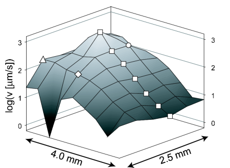
Figure 14: Velocity profile for a selected area near the pumping chip at a RF-power of 79 mW. The triangle, square and circle mark the positions at which the velocities shown in Fig. 13 were taken.

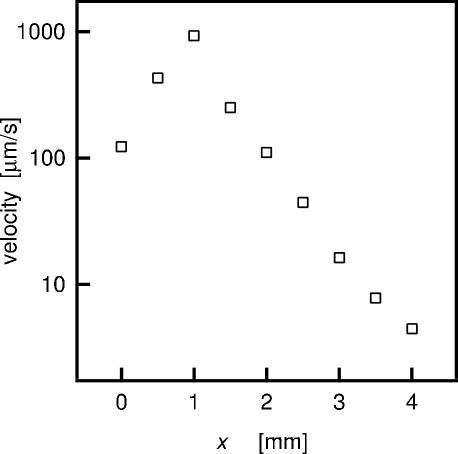
Figure 15: Velocity along the central x-direction at the positions shown by squares in Fig. 14. Ideally, the velocity at the symmetry point $x=0$ should vanish. The high gradient of the velocity field there and the experimental positional uncertainty, however, lead to the apparent finite velocity.

V Theory

V.1 Calculation of the flow field

All observed flows in the 200$\mu$m thick fluid film had velocities smaller than 1 mm/s and, hence, are characterized by Reynolds numbers smaller than 1. This means that the flow is completely laminar Brody et al. (1996), which simplifies the situation for the calculation of the streamlines. Although the detailed mechanism of the sound conversion into steady streaming is fairly complicated the steady flow is determined by the relatively simple Stokes equations Nyborg (1965) :

$$\mu\Delta{\bf v}({\bf x})=\nabla{p}({\bf x})-{\bf F}({\bf x})$$ (11)

$$\nabla\cdot{\bf v}=0$$ (12)

where $\mu$ denotes the shear viscosity of the fluid. The driving force ${\bf F}$ is given in terms of the sound wave by eq. (2). The SAW force field is generated in the area of the transducer and decays exponentially with distance. At about 1 mm it has dropped more than three orders of magnitude. We use these features in order to find an approximate analytical solution of eqs. (11) and (12) for the time averaged velocity and pressure fields and simplify the problem by the following assumptions: (i) lateral boundaries are neglected, i.e. we consider an infinitely extended fluid layer of thickness $d$ with no-slip boundary conditions at both confining plates; (ii) we approximate the actual spatially extended force density by a pair of constant forces being concentrated on lines perpendicular to the plates separated by the distance $a$:

$${\bf F}({\bf x})=\left({\bf f}_{+}\delta(x-a/2)+{\bf f}_{-}\delta(x+a/2)\right)\delta(y)$$ (13)

where $(x,y)={\bf r}$ are coordinates spanning the planes parallel to the plates and $z$ is a coordinate perpendicular to the plates with $z=0$ on lower and $z=d$ on the upper plate. The two forces ${\bf f}_{\pm}$ are assumed to have the same component in the $z$-direction and opposite components in the direction of the vector separating the two forces, i.e. in the $x$-direction, pushing the fluid away,

$${\bf f}_{\pm}=f_{z}{\bf e}_{z}\pm f{\bf e}_{x}.$$ (14)

where ${\bf e}_{x,z}$ are the unit vectors in $x$- and $z$-direction, respectively. We expect that outside the narrow spatial domain where the actual force does not vanish this presents a fairly good approximation to the actual situation. Because of the linearity of the Stokes equations (11,12) it is sufficient to consider a single line-force contribution. The final result can be obtained by the superposition of the solutions to the two forces.

Having only one line-force we may put the position of coordinate center at the position of the force. Further we note that one formally may include the $z$-component of the force into the pressure term by introducing the effective pressure

$$p_{\text{eff}}({\bf x})=\tilde{p}_{2}({\bf x})-f_{z}z\delta(x)\delta(y)$$ (15)

Measuring lengths, velocities and pressure in units of $d$, $f/\mu$ and $f/d$, respectively, leads to the dimensionless Stokes equations:

$$\Delta{\bf v}({\bf x})-\nabla p_{\text{eff}}({\bf x}) = -{\bf e}_{x}\delta^{2}({\bf r})$$ (16)

$$\nabla\cdot{\bf v}({\bf x})=0$$ (17)

with no-slip boundary conditions on the plates:

$${\bf v}({\bf r},0)={\bf v}({\bf r},1)=0$$ (18)

where $\delta^{2}({\bf r})=\delta(x)\delta(y)$ is a two-dimensional $\delta$-function. If one takes the divergence of the Stokes equation one finds a Poisson equation for the effective pressure:

$$\Delta p_{\text{eff}}({\bf x})=\frac{\partial}{\partial x}\delta^{2}({\bf r})$$ (19)

Because the inhomogeneity on the right hand side is $z$-independent it follows that the effective pressure also does not depend on $z$. Consequently the $z$-component of the velocity fulfills the Laplace equation with homogeneous boundary conditions and therefore $v_{z}({\bf x})$ vanishes everywhere. The remaining two components of the velocity field can be expressed in terms of a stream function $\Phi({\bf x})$:

$$v_{x}({\bf x})=\frac{\partial\Phi({\bf x})}{\partial y},\quad v_{y}({\bf x})=-\frac{\partial\Phi({\bf x})}{\partial x}$$ (20)

Differentiating the $x$- and $y$-components of the Stokes equation with respect to $y$ and $x$, respectively, and subtracting them one obtains for the stream function:

$$\Delta_{\bf r}\Delta\Phi({\bf x})=-\frac{\partial}{\partial y}\delta^{2}({\bf r})$$ (21)

where $\Delta_{\bf r}=\partial^{2}/\partial x^{2}+\partial^{2}/\partial y^{2}$ denotes the two-dimensional Laplace operator in the $(x,y)$-plane. Boundary conditions for $\Phi({\bf x})$ are:

$$\Phi({\bf r},0) = \Phi({\bf r},1)=0,$$ (22)

$$\frac{\partial\Phi({\bf x})}{\partial x} = \frac{\partial\Phi({\bf x})}{\partial y}=0$$ (23)

$$\lim_{r\to\infty}\Phi({\bf r},z) = 0$$ (24)

where $r=(x^{2}+y^{2})^{1/2}$ denotes the absolute value of ${\bf r}$. Because of the periodic boundary conditions with respect to $z$ the stream function can be represented as a $\sin$-series:

$$\Phi({\bf x})=\sum_{n=1}^{\infty}c_{n}({\bf r})\sin(\pi nz)$$ (25)

Here the coefficients are still functions of ${\bf r}$ and obey the equations

$$\Delta_{\bf r}\left(\Delta_{\bf r}-(\pi n)^{2}\right)c_{n}({\bf r})=-\gamma_{n}\frac{\partial}{\partial y}\delta({\bf r})$$ (26)

where

$$\gamma_{n}=2\int_{0}^{1}dz\>\sin(\pi nz)=\left\{\begin{array}[]{cl}0&\mbox{for $n$ even}\\ \frac{4}{\pi n}&\mbox{for $n$ odd}.\end{array}\right.$$ (27)

The solutions of these equations can be expressed in terms of the Green’s functions of the time-independent two-dimensional Klein-Gordon equation:

$$\left(\Delta_{\bf r}-k^{2}\right)g_{m}({\bf r})=\delta^{2}({\bf r})$$ (28)

where $k$ is a positive number. This Green’s function is given by Albeverio et al. (1988):

$$g_{k}({\bf r})=-\frac{1}{2\pi}K_{0}(kr)$$ (29)

where $K_{\nu}(z)$ is the modified Bessel function of order $\nu$, see Ref. Abramowitz and Stegun (1972). To achieve this goal we introduce an auxiliary function and rewrite eq. (26) in terms of two Klein-Gordon equations:

$$\Delta_{\bf r}h({\bf r}) = -\frac{\partial}{\partial y}\delta^{2}({\bf r})$$ (30)

$$\left(\Delta_{\bf r}-(n\pi)^{2})c_{n}({\bf r}\right) = \gamma_{n}h({\bf r})$$ (31)

The solution to the first equation can readily be expressed in terms of the Green’s function for $m=0$:

$$h({\bf r}) = -\lim_{m\to\infty}\frac{\partial}{\partial y}g_{m}({\bf r})$$ (32)

$$= \frac{1}{2\pi}\frac{\partial}{\partial y}\ln r$$

From the second equation one then finds:

$$c_{n}({\bf r}) = \gamma_{n}\int d^{2}{\bf r}^{\prime}\>g_{n\pi}({\bf r}-{\bf r}^{\prime})h({\bf r}^{\prime})$$ (33)

$$= \frac{\gamma_{n}}{(2\pi)^{2}}\frac{\partial}{\partial y}\int d^{2}{\bf r}^{\prime}\>K_{0}(n\pi r^{\prime})\ln|{\bf r}-{\bf r}^{\prime}|$$

Introducing polar coordinates one may perform the integration over ${\bf r}$ and obtains:

$$c_{n}({\bf r})=\left\{\begin{array}[]{ll}0&\text{for $n$ even}\\ \frac{2y}{n^{3}\pi^{4}r^{2}}\left(1-n\pi rK_{1}(n\pi r)\right)&\text{for $n$ odd}\end{array}\right.$$ (34)

The modified Bessel function decays rapidly for large values of its argument and therefore $n\pi rK_{1}(n\pi r)$ can be neglected for $\pi r\gg 1$. This gives the asymptotic behavior of the stream function:

$$\Phi_{\text{as}}({\bf x})=\frac{y}{4\pi r^{2}}z(1-z)$$ (35)

where we summed the sine-series $\sum_{n\;\text{odd}}\frac{\sin(n\pi)z}{n^{3}}=\frac{\pi^{3}}{8}z(1-z)$, see Ref. Bronsthein and Semendyayev (1985). Deviations from this asymptotic result can only be seen within a distance of a few gap widths from the location where the force is acting, see Figs. (16) and (17).

Figure 16: The streaming function $\Phi(0,y,0.5)$ (solid line) perpendicular to the axis $x=0$ displays extrema close to $|y|=0.3$. The broken line shows the asymptotic far field behavior according to eq. (35). Both functions perfectly coincide for distances from the origin that are larger than twice the plate distance.

Figure 17: The streaming function $\Phi(0,y,z)/\Phi(0,y,0.5)$ divided by its maximal value at $z=0.5$ at $x=0$ is shown as a function of the transversal coordinate $z$ for different distances $y$ from the origin where the force is sitting. In the very close vicinity of the force source, this profile is flat in the middle part of the fluid layer. For larger distances from the force it rapidly approaches the asymptotic parabolic profile, see eq. (35).

The streaming function of the force dipole readily follows as the linear combination of two velocity fields that are caused by slightly displaced line-forces pointing in opposite lateral directions:

$$\Phi_{\text{dipole}}({\bf x})=\Phi({\bf x}-{\bf e}\epsilon/2)-\Phi({\bf x}+{\bf e}\epsilon/2)$$ (36)

where $\epsilon$ is the width and ${\bf e}$ the unit vector in the direction of the displacement. In the following we will assume that both the displacement and the forces show in the $x$-direction. Using the asymptotic expression (35) and taking the leading contribution with respect to the distance $\epsilon$ one obtains:

$$\Phi^{\text{as}}_{\text{dipole}}=\epsilon\frac{yx}{8\pi r^{4}}z(1-z)$$ (37)

The velocity field then becomes asymptotically:

$$v_{x}^{as}({\bf x}) = \frac{\epsilon x}{8\pi r^{4}}\left(1-4\frac{y^{2}}{r^{2}}\right)z(1-z)$$

$$v_{y}^{as}({\bf x}) = -\>\frac{\epsilon y}{8\pi r^{4}}\left(1-4\frac{x^{2}}{r^{2}}\right)z(1-z)$$

$$v_{z}({\bf x}) = 0$$ (38)

Note that the near field has a less pronounced, logarithmic singularity. The full two-dimensional vector-field $v_{x}({\bf r},0.5),v_{y}({\bf r},0.5))$ that follows from the eqs.(20,25,34,36) is shown for a pair of opposite line force pointing in the positive and negative $x$-direction at ${\bf r}=(\pm 1,0)$ in Fig.18. In this case the fluid is sucked along the $y$-axis and pushed out in the $\pm x$-direction generating an eddy in each quadrant close to the dipole.

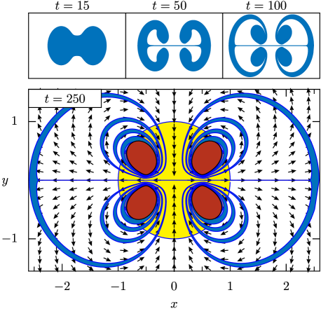
Figure 18: The graph shows the calculated evolution of a dye spot pumped by a SAW transducer in the center of the images. The black arrows mark the direction of the velocity field. The initial dye spot is marked by the circle. The 4 black ellipses in the lower image represent areas where the dye is trapped by an eddy. The trajectories were calculated for the plane in the middle of the fluid film with diffusion neglected.

V.2 Motion of advected particles

We consider the motion of a small particle that is advected by the flow field (38). Its trajectory agrees with the streamlines of the vector field ${\bf v}({\bf x})$ which are the solutions of

$$\dot{{\bf x}}(t)={\bf v}({\bf x}(t))$$ (39)

Because the velocity component in the $z$ direction vanishes the motion of a particle is strictly confined to the initial plane $z=z(0)$ as long as diffusion can be neglected. Fig. 18 shows the form that an initially circular spot in the central plane ($z=1/2$) acquires at four later times. We note that the area covered by the spot does not change because the vector field has vanishing divergence. The apparent change of the area of a dye spot which is observed in the experiment is due to the fact that different layers that move differently are superimposed. The alternating stripes of colored and uncolored fluid that evolve after sufficiently long time within each vertical layer cover each other and therefore cannot easily be seen in the experiment. In the course of time these layers become ever thinner and eventually diffusion becomes effective. Around the center of each of the four eddies regions exist that remain invariant under the flow, i.e. there is no transport out of these regions or into them other than diffusion.

Finally we consider a particle that initially sits in the middle position between the plates on the $x$-axis at a distance $x_{0}$ from the origin. It moves with the fluid strictly in the $x$-direction according to

$$\frac{d}{dt}x(t) = v_{x}(x(t),0,0.5)$$ (40)

$$= -\frac{c}{x(t)^{3}}$$

where $c=\epsilon/32\pi$ is a constant. The solution of this differential equation reads:

$$x(t)=\left(x_{0}^{4}+ct\right)^{1/4}$$ (41)

Here we have neglected the influence of diffusion. This will be of primary importance for the motion in the $z$ direction because there is no systematic force in this direction and, moreover, the $z$-coordinate of the particle position strongly influences its lateral velocity. A diffusional motion in the $z$-direction averages over $z$ and results in an effective value of the constant $c$ which becomes smaller by the factor 2/3.

In order to compare with the theoretical prediction of eq. (41) in Fig. 19 the fourth power of the position is plotted against time for four different RF-power values. Except for the highest power value where the asymptotic velocity field eq. (40) might not be fully applicable, the experimental data nicely fall onto straight lines. From the slope of this line we obtain the constant $c$ which determines the velocity field, eq. (40). The value of $c$ increases with the applied RF-power, see Fig. 20. An extrapolation of a linear fit of the data, however, would lead to a spurious finite positive value of $c$ and consequently to finite velocities in the absence of driving. We therefore conclude that the increase of $c$ with the RF-power must be weaker than linear.

Figure 19: The fourth power of the front positions (solid line) for four values of RF-power (10, 40, 63, 158 mW from bottom to top) of the dye spot indicated by the arrow in Fig. 6 measured at different instants of time (see also from Fig. 7) falls on straight lines as predicted by the asymptotic law given in eq. (41). Only for the very first points and at high RF-power deviations appear. From the inclination of the linear fits (broken lines) one obtains a reliable fit of the constant $c$ that determines the velocity field, see eq. (40).

Figure 20: The constant $c$ as determined from measurements of the position of the dye front is shown for different values of the RF-power.

VI Discussion

We applied fluorescence microscopy and FCS for the flow profile analysis of a SAW transducer in a 200$\mu$m thin fluid film. With the first technique the growth of the area of a Fluorescein spot was observed. From this the flow speed in x-direction could be determined.

In the FCS experiments, the flow speed in a homogeneous dispersion of fluorescent beads was measured at different points in a 5mm wide channel. With this technique no limitations exist for the choice of the position where the data is collected.

Both methods yield a fast decay of the flow speed with distance from the transducer with a comparable rate. As a theoretical model, the Navier Stokes equations were solved for an infinite fluid layer in the Stokes limit of low Reynolds numbers. The conversion of the sound wave into a steady flow was described in terms of body forces that were further simplified as line forces. Because the actual spatial extension of the body forces is confined to a narrow regime this seems to be a reasonable approximation. The resulting flow field is in good qualitative agreement with the experimental findings. According to the theoretical prediction, the velocity field asymptotically decays with the third inverse power of the distance from the IDT. The resulting motion of the front of a dye spot in the symmetry direction is in quantitative agreement with the measurements.

To determine the distance at which the influence of the transducer on the dye molecules vanishes, the growth speed ($v_{A}$) of the fluorescein covered area was measured. Plotting this data against the actual position of the advancing front shows also a fast decay until the diffusion constant of the the dye is reached. This distance depends logarithmically on the RF-power and is about 8 mm for the maximum applied 158 mW in the microscope study.

When the flow speed is measured at different points in the streamlines with both methods, a linear behavior dependent on the RF-power can be observed. However, when the constant $c$ in eq. (41) is determined from the $x$ position vs time data for different Hf-values, no line through the origin can be fitted. So following eq. (40) the flow speed cannot depend linearly on the power at a certain point in the flow field. The power range where measurements where taken, therefore probably represents an approximately linear regime.

Finally we address the question what one can learn from the presented experiments and theory in order to accelerate the hybridization of DNA in a thin fluid film with the lateral size of a normal glass slide (75x25mm). For this size, diffusive transport becomes extremely slow and should be complemented by advected transport. The flow induced by surface acoustic waves can be efficiently used for this purpose. However, because of the rapid decay of the induced velocity field away from the transducer the maximal mixing range was found to have a linear dimension of about 8 mm in the present experiment at the highest RF-power. A further increase of the power does not seem feasible because it would enlarge the mixing range only insignificantly. To account for the limited range of the induced flow by the SAW transducer the number of transducers on a slide should be increased. In the calculated flow field in Fig. 18 four eddies appear close to the transducer where particles can be trapped. To avoid this problem, pairs of transducers should always be operated alternately. So the trapped particles from one transducer will be moved by the other and vice versa.

References

- Kamholz and Yager (2001) A. Kamholz and P. Yager, Biophysical Journal 80, 4891 (2001).
- Darnton et al. (2001) N. Darnton, O. Bakajin, R. Huang, B. North, J. Tegenfeldt, E. Cox, J. Sturm, and R. Austin, Journal of Physcics: Condensed Matter 13, 4891 (2001).
- Wu and Keh (2003) J. Wu and H. Keh, Colloids and Surfaces A 212, 27 (2003).
- Zeng et al. (2001) S. Zeng, S. Chen, J. Mikkelsen, and J. Santiago, Sensors and Actuators B 79, 107 (2001).
- Maiti et al. (1997) S. Maiti, U. Haupts, and W. Webb, Proc. Acad. Sci. USA pp. 11753–11757 (1997).
- Shiokawa et al. (1989) S. Shiokawa, Y. Matsui, and T. Ueda, Ultrasonic Symposium pp. 643–646 (1989).
- Campbell and Jones (1970) J. Campbell and W. Jones, IEEE Transactions on Sensors and Ultrasonics 17, 71 (1970).
- Nyborg (1965) W. Nyborg, Physical Acoustics 2B, 265 (1965).
- Uchida et al. (1995) T. Uchida, T. Suzuki, and S. Shiokawa, IEEE Ultrasonic Symposium pp. 1081–1084 (1995).
- Magde et al. (1972) D. Magde, E. Elson, and W. Webb, Physical Review Letters 29, 705 (1972).
- Elson and Magde (1974) E. Elson and D. Magde, Biopolymers 13, 1 (1974).
- Magde et al. (1974) D. Magde, E. Elson, and W. Webb, Biopolymers 13, 29 (1974).
- Magde et al. (1978) D. Magde, W. Webb, and E. Elson, Biopolymers 17, 361 (1978).
- Rigler et al. (1992) R. Rigler, J. Widengren, and U. Mets, in Fluorescence Spectroscopy. New Methods and Applications, edited by O. Wolfbeis (Springer, Berlin, 1992).
- Schwille et al. (1997) P. Schwille, J. Bieschke, and F. Oehlenschlager, Biophysical Chemistry 66, 211 (1997).
- Krichevsky and Bonnet (2002) O. Krichevsky and G. Bonnet, Reports on Progress in Physics 65, 251 (2002).
- Thompson et al. (2002) N. L. Thompson, A. M. Lieto, and N. W. Allen, Current Opinion in Structural Biology 12, 634 (2002).
- Hess and Webb (2002) S. Hess and W. Webb, Biophysical Journal 83, 2300 (2002).
- Gösch et al. (2000) M. Gösch, H. Blom, T. Heino, and R. R., Analytical Chemistry 72, 3260 (2000).
- Eigen and Rigler (1994) M. Eigen and R. Rigler, Proceedings of the National Academy of Sciences of the United States of America 91, 5740 (1994).
- Starchev et al. (1998) K. Starchev, J. W. Zhang, and J. Buffle, Journal of Colloid and Interface Science 203, 189 (1998).
- Starchev et al. (1999) K. Starchev, J. Buffle, and E. Perez, Journal of Colloid and Interface Science 213, 479 (1999).
- Brody et al. (1996) J. Brody, P. Yager, R. Goldstein, and R. Austin, Biophysical Journal 71, 3430 (1996).
- Albeverio et al. (1988) S. Albeverio, F. Gesztesy, R. Høegh-Krohn, and H. Holden, Solvable Models in Quantum Mechanics (Springer-Verlag, Berlin, 1988).
- Abramowitz and Stegun (1972) M. Abramowitz and I. Stegun, Handbook of Mathematical Functions (Dover Publications, New York, 1972).
- Bronsthein and Semendyayev (1985) I. Bronsthein and K. Semendyayev, Handbook of Mathematics (van Nostrand Reinhold Company, New York, 1985).