Crossover from Non–Equilibrium to Equilibrium Behavior in the Time–Dependent Kondo Model

Abstract

We investigate the equilibration of a Kondo model that is initially prepared in a non–equilibrium state towards its equilibrium behavior. Such initial non–equilibrium states can e.g. be realized in quantum dot experiments with time–dependent gate voltages. We evaluate the non–equilibrium spin–spin correlation function at the Toulouse point of the Kondo model exactly and analyze the crossover between non–equilibrium and equilibrium behavior as the non–equilibrium initial state evolves as a function of the waiting time for the first spin measurement. Using the flow equation method we extend these results to the experimentally relevant limit of small Kondo couplings.

Introduction.– Equilibration in non–perturbative many–body problems is not well–understood with many fundamental questions still being unanswered. For example the crossover from a non–equilibrium initial state to equilibrium behavior after a sufficiently long waiting time poses many interesting questions that are both experimentally relevant and theoretically of fundamental importance. From the experimental side there is currrent interest in such questions related to transport experiments in quantum dots. Non–perturbative Kondo physics has been observed in quantum dots QuantumDots and given rise to a wealth of experimental and theoretical investigations. Quantum dot experiments allow the possibility to systematically study the effect of time–dependent parameters, like switching on the Kondo coupling at a specific time and measuring the time–dependent current. From the theoretical point of view this is related to studying the time–dependent buildup of the non–perturbative Kondo effect.

The combination of strong–coupling behavior and time–dependent parameters makes such problems theoretically very challenging. Various methods like time–dependent NCA and renormalized perturbation theory Nordlander , the numerical renormalization group Costi , bosonization and refermionization techniques Schiller , etc.  have allowed insights and e.g. identified the time scale $t_{\rm K}\propto\hbar/k_{\rm B}T_{\rm K}$ related to the Kondo temperature $T_{\rm K}$ with the relevant time scale for the buildup of the Kondo resonance. Using the form factor approach Lesage and Saleur could derive exact results for the spin expectation value $P(t)=\langle S_{z}(t)\rangle$ for a product initial state Lesage . However, no exact results are available regarding the crossover from non–equilibrium to equilibrium behavior in this paradigm strong–coupling model of condensed matter theory.

In this Letter we use bosonization and refermionization techniques to calculate the zero temperature spin–spin correlation function of the Kondo model at the Toulouse point Toulouse exactly for two non–equilibrium preparations: I) The impurity spin is frozen for time $t<0$. II) The impurity spin is decoupled from the Fermi sea for time $t<0$. We find a crossover between non–equilibrium exponential decay and equilibrium algebraic decay as one increases the waiting time for measuring the spin–spin correlation function at time $t>0$. One concludes that zero temperature equilibration occurs exponentially fast with a time scale set by the inverse Kondo temperature, and a mixture of non–equilibrium and equilibrium behavior for finite waiting times. Using the flow equation solution of the Kondo model Hofstetter ; Slezak we then extend these results away from the Toulouse point to the experimentally relevant limit of small Kondo couplings in a systematic approximation.

Model.– The Kondo model describes the interaction of a spin–1/2 degree of freedom $\vec{S}$ with a Fermi sea

$$H=\sum_{k,\alpha}\epsilon_{k}c^{\dagger}_{k\alpha}c^{\phantom{\dagger}}_{k\alpha}+\sum_{i}J_{i}\sum_{\alpha,\beta}c^{\dagger}_{0\alpha}\,S^{\phantom{\dagger}}_{i}\,\sigma^{\alpha\beta}_{i}\>c^{\phantom{\dagger}}_{0\beta}\ .$$ (1)

Here $c^{\dagger}_{0\alpha},c^{\phantom{\dagger}}_{0\alpha}$ is the localized electron orbital at the impurity site. We allow for anisotropic couplings $J_{i}=(J_{\bot},J_{\bot},J_{\|})$ and consider a linear dispersion relation $\epsilon_{k}=v_{F}\,k$. Throughout this Letter we are interested in the universal behavior in the scaling limit $J_{\bot}/v_{F}\rightarrow 0$. The Kondo Hamiltonian can be mapped to the spin–boson model, which is the paradigm model of dissipative quantum mechanics Leggett . Our results can be interpreted in both these model settings; in the sequel we will focus on the Kondo model interpretation.

We study two non–equilibrium preparations: I) The impurity spin is frozen for time $t<0$ by a large magnetic field term $h(t)S_{z}$ that is switched off at $t=0$: $h(t)\gg T_{\rm K}$ for $t<0$ and $h(t)=0$ for $t\geq 0$. II) The impurity spin is decoupled from the bath degrees of freedom for time $t<0$ (like in situation I we assume $\langle S_{z}(t\leq 0)\rangle=+1/2$) and then the coupling is switched on at $t=0$: $J_{i}(t)=0$ for $t<0$ and $J_{i}(t)=J_{i}>0$ time–independent for $t\geq 0$. This situation is of particular interest in future quantum dot experiments where the quantum dot is suddenly switched into the Kondo regime by applying a time–dependent voltage on a nearby gate Nordlander .

The difference between these two initial states is that in I) the electrons are in equilibrium with respect to the potential scattering induced by the frozen spin for $t<0$. On the other hand in II) the initial state of the electrons is an unperturbed Fermi sea. We will later see that both initial states lead to the same spin dynamics.

A suitable quantity for studying equilibration is the symmetrized zero temperature spin–spin correlation function $C_{\rm I,II}(t_{w},t)\stackrel{{\scriptstyle\rm def}}{{=}}\frac{1}{2}\langle\{S_{z}(t_{w}),S_{z}(t_{w}+t)\}\rangle_{\rm I,II}$. In equilibrium this correlation function exhibits its well–known $t^{-2}$-algebraic long time decay Leggett and is, of course, independent from the initial (waiting) time $t_{w}$: $C_{\rm eq}(t)=C_{\rm eq}(t_{w},t)\propto t^{-2}$.

Exact results for the non–equilibrium spin dynamics have so far only been obtained for the spin expectation value $P(t)\stackrel{{\scriptstyle\rm def}}{{=}}\langle S_{z}(t)\rangle$. At the Toulouse point $J_{\|}^{\rm TP}/2\pi v_{F}=1-1/\sqrt{2}$ Toulouse $P(t)$ can be evaluated exactly Leggett and one finds a purely exponential decay $P(t)=\frac{1}{2}\exp(-2t/\pi wt_{\rm K})$. Here and in the sequel, we define the Kondo time scale as $t_{\rm K}=1/T_{\rm K}$ with the Kondo temperature defined via the impurity contribution to the Sommerfeld coefficient $\gamma_{\rm imp}=w\pi^{2}/3T_{\rm K}$, where $w=0.4128$ is the Wilson number. Using the form factor approach Lesage and Saleur could derive exact results for $P(t)$ even away from the Toulouse point Lesage . For $0<J_{\|}<J_{\|}^{\rm TP}$ they find that the spin expectation value again decays exponentially for large times $t/t_{\rm K}\gg 1$ with the same exponential dependence $P(t)\propto\exp(-2t/\pi wt_{\rm K})$, however, its behavior at finite times is more complicated.

Since $P(t)=2C(t_{w}=0,t)$ these results raise the question of how the crossover between non–equilibrium exponential decay and equilibrium algebraic decay occurs as a function of the waiting time $t_{w}$.

Toulouse point.– We have addressed this issue by evaluating $C_{\rm I,II}(t_{w},t)$ exactly at the Toulouse point of the model. One finds that the result is the same in both situation I) and II):

$$C_{\rm I,II}(t_{w},t) = C_{\rm eq}(t)$$ (2)

$$-2e^{-t_{w}/t_{\rm B}}s(t)\big{(}s(t_{w})e^{-t/t_{\rm B}}-s(t_{w}+t)\big{)}$$

$$-e^{-2t_{w}/t_{\rm B}}\big{(}s(t_{w})e^{-t/t_{\rm B}}-s(t_{w}+t)\big{)}^{2}$$

for $t,t_{w}\geq 0$. Here $s(\tau)=(t_{\rm B}/\pi)\int_{0}^{\infty}d\omega\,\sin(\omega\tau)/(1+\omega^{2}t_{\rm B}^{2})$ with the abbreviation $t_{\rm B}\stackrel{{\scriptstyle\rm def}}{{=}}\pi wt_{\rm K}$. In terms of $s(\tau)$ the equilibrium correlation function reads

$$C_{\rm eq}(t)=\frac{1}{4}\,e^{-2t/t_{\rm B}}-s^{2}(t)\ .$$ (3)

Notice that $s(t)\simeq t_{\rm B}/\pi t$ for $t\gg t_{\rm B}$ leading to the algebraic long-time decay. Therefore the Fourier transform of the equilibrium correlation function is proportional to $|\omega|$ for small frequencies $\omega/T_{\rm K}\ll 1$: $C_{\rm eq}(\omega)\propto|\omega|/T_{\rm K}^{2}$.

For zero waiting time $t_{w}=0$ the non-equilibrium correlation function Eq. (2) shows the well–known purely exponential decay $C_{\rm I,II}(t_{w}=0,t)=\frac{1}{4}e^{-2t/t_{\rm B}}$, while for any fixed $t_{w}>0$ the algebraic long time behavior dominates with an amplitude that is suppressed depending on the waiting time:

$$C_{\rm I,II}(t_{w},t)\simeq-s^{2}(t)\,\left(1-e^{-t_{w}/t_{\rm B}}\right)^{2}+O\left(\left(t_{\rm B}/t\right)^{3}\right)$$ (4)

for $t\gg{\rm max}(t_{w},t_{\rm B})$. In particular, one can read off from (2) that the difference between the non–equilibrium and equilibrium correlation function decays exponentially fast as a function of the waiting time

$$|C_{\rm I,II}(t_{w},t)-C_{\rm eq}(t)|\propto e^{-t_{w}/t_{\rm B}}$$ (5)

for $t_{w}\gg t_{\rm B}$. These results can be understood by noticing that the initial state corresponds to an excited state of the model, therefore yielding a different spin dynamics from equilibrium. After a time scale of order $t_{\rm K}$ corresponding to the low–energy scale of the model, the initial non–equilibrium state leads to the behavior of the equilibrium ground state with deviations that decay exponentially fast as one increases the waiting time note . This crossover behavior of the non-equilibrium correlation function at the Toulouse point is shown in Fig. 1 for the one–sided Fourier transform with respect to the time difference $t$

$$C(t_{w},\omega)=\int_{-\infty}^{\infty}\frac{dt}{2\pi}\>e^{i\omega t}\>C(t_{w},|t|)\ .$$ (6)

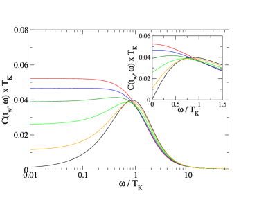
Figure 1: Universal curves for the spin–spin correlation function $C(t_{w},\omega)$ at the Toulouse point for various waiting times ($t_{w}=0,t_{\rm K}/4,t_{\rm K}/2,t_{\rm K},2t_{\rm K},\infty$ from top to bottom). The inset depicts the same curves on a linear scale, which shows more clearly the onset of the non–analyticity ($C(t_{w},\omega)-C(t_{w},0)\propto|\omega|$) for waiting times $t_{w}>0$ leading to the algebraic long–time decay.

Method.– We perform the standard procedure of bosonizing the Kondo Hamiltonian in terms of spin–density excitations $b^{\phantom{\dagger}}_{k},b^{\dagger}_{k}$, and then eliminating its $J_{\|}$–coupling using a polaron transformation $U=\exp[i\delta\,S_{z}\,\sum_{k>0}(1/\sqrt{k})\,(b^{\phantom{\dagger}}_{k}-b^{\dagger}_{k})]$ (for details see e.g. Leggett ). At the Toulouse point the transformed Hamiltonian $\tilde{H}=U^{\dagger}HU$ can be refermionized Leggett

$$\tilde{H}=\sum_{k}\epsilon_{k}\Psi^{\dagger}_{k}\Psi^{\phantom{\dagger}}_{k}+\sum_{k}V_{k}\left(\Psi^{\dagger}_{k}d+d^{\dagger}\Psi^{\phantom{\dagger}}_{k}\right)\ .$$ (7)

Here the spinless fermions $\Psi(x)$ correspond to soliton excitations built from the bosonic spin–density waves with the refermionization identity $\Psi(x)\propto\exp\big{[}i\sum_{k>0}(1/\sqrt{k})\,(b^{\phantom{\dagger}}_{k}e^{-ikx}-b^{\dagger}_{k}e^{ikx})\big{]}$. Eq. (7) can be interpreted as a resonant level model with the hybridization function $\Delta(\epsilon)\stackrel{{\scriptstyle\rm def}}{{=}}\pi\sum_{k}V_{k}^{2}\delta(\epsilon-\epsilon_{k})=T_{K}/\pi w$ and a fermionic impurity orbital $d$ with the identity $S_{z}=d^{\dagger}d-1/2$. Model I is therefore represented by a resonant level model with a time–dependent impurity orbital energy $\epsilon_{d}(t)=h(t)$

$$\tilde{H}_{\rm I}(t) = \sum_{k}\epsilon_{k}\Psi^{\dagger}_{k}\Psi^{\phantom{\dagger}}_{k}+\epsilon_{d}(t)\,(d^{\dagger}d-1/2)$$ (8)

$$+\sum_{k}V_{k}\left(\Psi^{\dagger}_{k}d+d^{\dagger}\Psi^{\phantom{\dagger}}_{k}\right)$$

with $\epsilon_{d}(t<0)=\infty$, $\epsilon_{d}(t\geq 0)=0$. In model II the spin is not coupled to the Fermi sea for time $t<0$: this leads to a time–dependent hybridization function and a time–dependent potential scattering term (due to the polaron transformation $U$)

$$\tilde{H}_{\rm II}(t) = \sum_{k}\epsilon_{k}\Psi^{\dagger}_{k}\Psi^{\phantom{\dagger}}_{k}+\sum_{k}V_{k}(t)\left(\Psi^{\dagger}_{k}d+d^{\dagger}\Psi^{\phantom{\dagger}}_{k}\right)$$ (9)

$$+\langle S_{z}(t=0)\rangle\sum_{k,k`}g_{kk^{\prime}}(t)(\Psi^{\dagger}_{k}\Psi^{\phantom{\dagger}}_{k^{\prime}}-1/2)$$

with $g_{kk^{\prime}}(t<0)=(1-\sqrt{2})/2\pi v_{F}$, $g_{kk^{\prime}}(t\geq 0)=0$ and $\Delta(\epsilon;t<0)=0$, $\Delta(\epsilon;t\geq 0)=T_{K}/\pi w$.

In order to evaluate the non–equilibrium spin dynamics we use the quadratic form of $\tilde{H}_{\rm I,II}$ to solve the Heisenberg equations of motion for the operators $d^{\dagger}(t),d(t)$ exactly. After some straightforward algebra one can write the operator $S_{z}(t)$ for $t>0$ as a quadratic expression in terms of the operators $\Psi^{\dagger}_{k}(t=0)$, $\Psi^{\phantom{\dagger}}_{k}(t=0)$, $d^{\dagger}(t=0)$ and $d(t=0)$ at time $t=0$ long_paper . The non–equilibrium correlation function is then given by

$$C_{\rm I,II}(t_{w},t)=\frac{1}{2}\langle\tilde{G}_{\rm I,II}|\{S_{z}(t_{w}),S_{z}(t_{w}+t)\}|\tilde{G}_{\rm I,II}\rangle\ .$$ (10)

where we insert the solution of the Heisenberg equation of motion for $S_{z}(t)$. The initial non–equilibrium states $|\rm\tilde{G}_{\rm I,II}\rangle$ remain time–independent in the Heisenberg picture and are simply the ground states of the Hamiltonians $\tilde{H}_{\rm I,II}(t)$ for time $t<0$. Inserting these expressions in (10) yields (2) after some tedious but straightforward algebra long_paper . For completeness we also give the result for the imaginary part of the non–equilibrium Greens function

$$\!\!\!K_{\rm I,II}(t_{w},t)\stackrel{{\scriptstyle\rm def}}{{=}}\frac{1}{2}\,\langle\,[S_{z}(t_{w}),S_{z}(t_{w}+t)]\,\rangle_{\rm I,II}$$ (11)

$$\!\!\!=-i\,e^{-t/t_{\rm B}}(s(t)-s(t_{w}+t)e^{-t_{w}/t_{\rm B}}+s(t_{w})e^{-(t_{w}+t)/t_{\rm B}})$$

which again approaches the equilibrium result $K_{\rm eq}(t)=-i\,e^{-t/t_{\rm B}}s(t)$ exponentially fast as a function of $t_{w}/t_{\rm B}$.

Kondo limit.– The Toulouse point exhibits many universal features of the strong–coupling phase of the Kondo model like local Fermi liquid properties, however, other universal properties like the Wilson ratio depend explicitly on the coupling $J_{\parallel}$. This raises the question which of the above non–equilibrium to equilibrium crossover properties are generic in the strong–coupling phase. We investigate this question by using the flow equation method Wegner that allows us to extend our analysis away from the Toulouse point in a controlled expansion. In this Letter we focus on the experimentally most relevant limit of small Kondo couplings (notice that the flow equation approach is not restricted to this limit and can be used for general $J_{\|}$ prb ).

The flow equation method diagonalizes a many–particle Hamiltonian through a sequence of infinitesimal unitary transformations in a systematic approximation Wegner . This approach was carried through for the Kondo model in Ref. Hofstetter . Since the Hamiltonian is transformed into its diagonal basis, we can follow the same steps as in the Toulouse point analysis: i) The Heisenberg equations of motion for the unitarily transformed observables can be solved easily with respect to the diagonal Hamiltonian. ii) One then re-expresses the time–evolved operators through the operators in the initial (non–diagonal) basis for time $t=0$. iii) The correlation functions (10) for general $t_{w}$ are evaluated. An operator product expansion to leading order is employed like in Ref. Hofstetter to close the resulting systems of equations.

The above procedure can be used quite generally to apply the flow equation method to time–dependent Hamiltonians of the above kind. For the Kondo model specifically, one can simplify the calculation by using the results from Ref. Slezak : it was shown that a resonant level model (7) with a universal non–trivial hybridization function $\Delta_{\rm eff}(\epsilon)\neq$ const. can be used as an effective model for the spin dynamics on all time scales; the only free parameter is the low–energy scale $T_{K}$. Similarly, the effective Hamiltonian (9) with $\Delta(\epsilon;t>0)=\Delta_{\rm eff}(\epsilon)$ from Ref. Slezak yields the $S_{z}$–spin dynamics for both non–equilibrium situations I and II. A careful analysis prb shows that the only effect not captured by the resonant level model is the polaron–like transformation that is contained in the complete flow equation approach. This polaron tranformation leads to an initial potential scattering term like in (9) with $g_{kk^{\prime}}(t<0)=(\lambda(B_{\rm eff})-\sqrt{2})/2\pi v_{F}$, where $B_{\rm eff}=1/(\epsilon_{k}^{2}+\epsilon_{k^{\prime}}^{2})$ and $\lambda(B)$ is the flowing scaling dimension according to Ref. Hofstetter ($\lambda(B=0)=\sqrt{2}$ and $\lambda(B\rightarrow\infty)=1$). However, this initial potential scattering term has a neglible effect (relative error $<5\%$) unless one is interested in short waiting times $t_{w}\lesssim t_{\rm K}/4$: for larger waiting times the effective Hamiltonian from Ref. Slezak yields a very accurate description without the need for the full flow equation analysis.

From the quadratic Hamiltonian (9) with the above effective coupling constants (including the initial potential scattering term) one can easily evaluate the non–equilibrium correlation functions; results are depicted in Fig. 2. The key observations from the Toulouse point analysis hold in the Kondo limit as well, only the crossover behavior is more complicated: 1) The system approaches equilibrium behavior exponentially fast as a function of $t_{w}/t_{\rm K}$ (compare Eq. (5)). Notice that the initial approach for small $t_{w}$ in Fig. 2 is faster than at the Toulouse point (Fig. 1). 2) An algebraic long–time decay $\propto t^{-2}$ dominates for all nonzero waiting times $t_{w}>0$ (compare Eq. (4)).

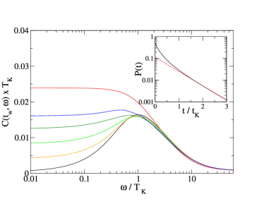
Figure 2: Universal curves for the spin–spin correlation function $C(t_{w},\omega)$ in the limit of small Kondo couplings (Kondo limit) for various waiting times ($t_{w}=0,t_{\rm K}/4,t_{\rm K}/2,t_{\rm K},2t_{\rm K},\infty$ from top to bottom like in Fig. 1). The inset shows the spin expectation value $P(t)$: the dashed line is an asymptotic fit $P_{\rm asym}(t)=0.11\exp(-1.51\,t/t_{\rm K})$.

For zero waiting time $t_{w}=0$ the inset in Fig. 2 shows the decay of the spin expectation value $P(t)$ in the Kondo limit, which has not been previously calculated explicitly on all time scales. For large $t/t_{\rm K}$ the behavior crosses over into an exponential decay which agrees very well with the exact asymptotic result from Ref. Lesage : $P_{\rm exact}(t)\propto\exp(-2t/\pi wt_{\rm K})\propto\exp(-1.54t/t_{\rm K})$. On shorter time scales the decay is faster, which is due to unrenormalized coupling constants at large energies that dominate the short–time behavior.

Conclusions.– Summing up, we have investigated the crossover to equilibrium behavior for a Kondo model that is prepared in an initial non–equilibrium state. We calculated the non–equilibrium spin–spin correlation function on all time scales and could show that it evolves exponentially fast towards its equilibrium form for large waiting time of the first spin measurement $t_{w}\gg t_{\rm K}$, see Eq. (5). Our results also established that the flow equation method is a very suitable approach for studying such non–equilibrium problems: it agrees with very good accuracy with exact results for both $t_{w}=0$ and $t_{w}=\infty$, and can describe the crossover regime as well.

Finally, it is worthwile to recall the fundamental quantum mechanical observation that the overlap between the time–evolved non–equilibrium state and the true ground state of the Kondo model is always time–independent. Therefore it is not strictly accurate to conclude from our results that an initial non–equilibrium state ”decays” into the ground state: rather, quantum observables which exhibit equilibration behavior are probes for which the time–evolved initial non–equilibrium state eventually ”looks like” the ground state. Since the notion of equilibration into the ground state plays a fundamental role in quantum physics, it would be very interesting to study other systems with quantum dissipation to see which of the crossover and equilibration properties derived in this Letter are generic.

We acknowledge valuable discussions with T. Costi and D. Vollhardt. This work was supported through SFB 484 of the Deutsche Forschungsgemeinschaft (DFG). SK acknowledges support through a Heisenberg fellowship of the DFG.

References

- (1) D. Goldhaber-Gordon, et al., Nature 391, 156 (1998); S. M. Cronenwett, T. H. Oosterkamp, and L. P. Kouwenhoven, Science 281, 540 (1998).
- (2) P. Nordlander, M. Pustilnik, Y. Meir, N. S. Wingreen, and D. C. Langreth, Phys. Rev. Lett. 83, 808 (1999); P. Nordlander, N. S. Wingreen, Y. Meir, and D. C. Langreth Phys. Rev. B 61, 2146 (2000); M. Plihal, D. C. Langreth, and P. Nordlander, Phys. Rev. B 61, R13341 (2000).
- (3) T. Costi, Phys. Rev. B 55, 3003 (1997).
- (4) A. Schiller and S. Hershfield, Phys. Rev. B 62, R16271 (2000).
- (5) F. Lesage and H. Saleur, Phys. Rev. Lett. 80, 4370 (1998).
- (6) G. Toulouse, C. R. Acad. Sci. Paris 268, 1200 (1969).
- (7) W. Hofstetter and S. Kehrein, Phys. Rev. B 63, 140402(R) (2001).
- (8) C. Slezak, S. Kehrein, Th. Pruschke, and M. Jarrell, Phys. Rev. B 67, 184408 (2003).
- (9) A. J. Leggett, S. Chakravarty, A. T. Dorsey, M. P. A. Fisher, A. Garg, and W. Zwerger, Rev. Mod. Phys. 59, 1 (1987).
- (10) Notice that it is not possible to think of the time–evolved initial non–equilibrium state as effectively being equivalent to an equilibrium system with a nonzero temperature that depends on the waiting time : nonzero temperature leads to an exponential decay and not to the correct algebraic long–time behavior for in (4).
- (11) Details of this calculation will be published elsewhere: it conceptually follows the exact evaluation of for an impurity in a Luttinger liquid by J. von Delft and H. Schoeller, Ann. Physik (Leipzig) 4, 225 (1998).
- (12) F. Wegner, Ann. Physik (Leipzig) 3, 77 (1994).
- (13) Details of the flow equation analysis will be published separately.