On leave from ] Petersburg Nuclear Physics Institute, Gatchina 188300, Russia.

The Hall conductivity in unconventional charge density wave systems

Abstract

Charge density waves with unconventional order parameters, for instance, with d-wave symmetry (DDW), may be relevant in the underdoped regime of high-T_c cuprates or other quasi-one or two dimensional metals. A DDW state is characterized by two branches of low-lying electronic excitations. The resulting quantum mechanical current has an inter-branch component which leads to an additional mass term in the expression for the Hall conductivity. This extra mass term is parametrically enhanced near the “hot spots” of fermionic dispersion and is non-neglegible as is shown by numerical calculations of the Hall number in the DDW state.

Recently, the interest in charge density waves with unconventional order parameters has increasedMaki ; Neto ; Cappelluti ; Chakravarty . In particular, it has been shown that a charge density wave with d-wave symmetry (DDW) represents a stable state of the $t-J$ model in the large-N limit in certain doping and temperature regionsCappelluti . It thus may be intimately related to the pseudogap phase of high-T_c superconductorsCappelluti ; Chakravarty . The presence of a DDW state should also cause changes in transport coefficientsWKim02 . Refs.Chakravarty02 ; Norman03 discuss DDW-induced changes in the Hall effect on the basis of the standard formulaZiman , which is applicable to an usual metal. In the present paper we argue that a careful reconsideration of the Hall coefficient for the case of a DDW state results in an additional term to the usual expression. This term enhances the change in the Hall number due to onset of a DDW order parameter.

Qualitatively, the appearance of the new term can be understood as follows. It is known from the band theory of metals that the quantum mechanical current operator consists of two parts, the intra-band derivative with respect to the wave vector and the term describing the interband transitions. Usually, the interband energy spacing is large enough to neglect the influence of the interband current term.

In the DDW state the situation is different. The charge density wave with momentum $\bf Q$ couples electrons which differ in momentum by $\bf Q$. Taking, for instance, a square lattice and ${\bf Q}={(\pi,\pi)}$ a two-band picture is obtained in the reduced magnetic Brillouin zone. There exists regions around certain wave vectors ${\bf K}$, the so-called “hot-spots”, where the quasi-particle energies of both bands are close to the Fermi level. The influence of these hot spots determines the changes in the Hall conductivity, as shown in Ref.Chakravarty02 . We find that the interband contribution to the current is particularly important in the vicinity of the hot spots, leading to significant changes in the theoretical predictions.

From a broader viewpoint, the necessity of inclusion of the interband current terms is known for the case of almost degenerate electron spectra LL9 and for the case of the electromagnetic response in nodal (d-wave) superconductors. On a formal level, it can be illustrated as follows. Near the point of degeneracy, ${\bf K}$, the spectrum can be represented as $\epsilon_{{\bf k}+{\bf K}}\sim\sqrt{k_{x}^{2}+k_{y}^{2}}$. The inclusion of the external vector potential through the Peierls substitution, ${\bf k}\to{\bf k}-e{\bf A}$, leads to a troublesome non-analyticity of the fermionic action on ${\bf A}$, i.e. $\sqrt{|{\bf A}|^{2}}$. The recipe for the correct treatment of the electromagnetic response in such cases is well knownLL9 . It amounts to retaining the non-diagonal form of the Hamiltonian, which is analytic in ${\bf A}$ and contains the interband currents, until the end of the calculation.

The mean-field Hamiltonian in the DDW state is

$${\cal H} = \sum_{{\bf k},\sigma}\left[\xi_{\bf k}a^{\dagger}_{{\bf k}\sigma}a_{{\bf k}\sigma}+i\Delta_{\bf k}a^{\dagger}_{{\bf k}\sigma}a_{{\bf k}+{\bf Q},\sigma}+h.c.\right]$$ (1)

Taking nearest and next-nearest neighbor hoppings $t$ and $t^{\prime}$ into account and putting the lattice constant of the square lattice to unity, the electronic dispersion is $\xi_{\bf k}=-2t(\cos k_{x}+\cos k_{y})+4t^{\prime}\cos k_{x}\cos k_{y}-\mu$. In the following we also will use the abbreviations $\xi_{\pm}=(\xi_{\bf k}\pm\xi_{{\bf k}+{\bf Q}})/2$. The d-density wave the order parameter is of the form $\Delta_{\bf k}=\Delta_{0}(\cos k_{x}-\cos k_{y})=-\Delta_{{\bf k}+{\bf Q}}$.

In terms of two-component fermion operator $\Psi^{\dagger}_{{\bf k}\sigma}=\left(a^{\dagger}_{{\bf k}\sigma},a^{\dagger}_{{\bf k}+{\bf Q},\sigma}\right)$ the Hamiltonian becomes ${\cal H}=\sum_{{\bf k},\sigma}\Psi^{\dagger}_{{\bf k}\sigma}{\hat{H}}_{{\bf k}}\Psi_{{\bf k}\sigma}$ with

$${\hat{H}}_{{\bf k}}=\begin{pmatrix}\xi_{\bf k}&i\Delta_{\bf k}\\ -i\Delta_{\bf k}&\xi_{{\bf k}+{\bf Q}}\end{pmatrix}.$$ (2)

It can be diagonalized by the unitary transformation $U=\exp i\sigma^{1}\theta_{\bf k}$ with

$$\theta_{\bf k}=(1/2)\arctan(\Delta_{\bf k}/\xi_{-}),$$

where $\sigma^{i}$ denote the Pauli matrices. We have $U\hat{H}U^{\dagger}=diag(\varepsilon_{1},\varepsilon_{2})\equiv\hat{h}$ and the new quasiparticle energies are

$$\varepsilon_{1,2}=\xi_{+}\pm\left[\xi_{-}^{2}+\Delta_{\bf k}^{2}\right]^{1/2}.$$ (3)

The fermionic Green’s function is given by

$${\hat{G}}_{{\bf k}\sigma}(i\omega) = \left(i\omega-\hat{H}\right)^{-1},$$ (4)

and it is diagonalized by the same matrix $U$. We write ${\hat{G}}=U^{\dagger}\hat{g}U$ with $\hat{g}=(\omega-\hat{h})^{-1}$. The external vector potential is included into the Hamiltonian by the Peierls substitution ${\hat{H}}_{{\bf k}}\to{\hat{H}}_{{\bf k}-e{\bf A}}.$

In what follows we use the Kubo approach within the linear response theory. It expresses the d.c.  conductivity tensor, $\sigma_{\alpha\beta}$, in terms of the current-current correlation function, in the limit of static uniform external fields. Mahan In case of point-like impurity scattering, allowing the neglectance of the vertex corrections to the corresponding diagrams, the standard derivation leads to the following formula

$$\sigma_{\alpha\beta}=-e^{2}\int\frac{dxd{\bf k}}{(2\pi)^{3}}\frac{\partial n(x)}{\partial x}{\rm Tr}\left[{\hat{V}}_{{\bf k}}^{\alpha}{\hat{G}}^{A}_{{\bf k}}(x){\hat{V}}_{{\bf k}}^{\beta}{\hat{G}}^{R}_{{\bf k}}(x)\right],$$ (5)

where $n(x)=(e^{x/T}+1)^{-1}$ is the Fermi function, the summation over the spin index has been performed, and the integration over ${\bf k}$ refers to the magnetic Brillouin zone in order to avoid double counting. Here ${\hat{G}}^{A(R)}$ denote the advanced (retarded) Green’s function defined on the real energy axis $x$. The group velocity, corresponding to the microscopic quantum-mechanical current, is

$${\hat{V}}_{{\bf k}}^{\alpha}={\partial{\hat{H}}_{{\bf k}}}/{\partial k_{\alpha}}\equiv\partial^{\alpha}{\hat{H}}_{{\bf k}}.$$ (6)

Using the above definitions the expression for the conductivity can be rewritten as ${\rm Tr}\left[{\hat{V}}^{\alpha}{\hat{G}}^{A}{\hat{V}}^{\beta}{\hat{G}}^{R}\right]={\rm Tr}\left[{\hat{v}}^{\alpha}{\hat{g}}^{A}{\hat{v}}^{\beta}{\hat{g}}^{R}\right]$ with ${\hat{v}}^{\alpha}=U^{\dagger}{\hat{V}}^{\alpha}U$ and

$${\hat{v}}^{\alpha}=\partial^{\alpha}\hat{h}+[(U^{\dagger}\partial^{\alpha}U),\hat{h}]\equiv{\cal D}^{\alpha}\hat{h}.$$

The last equation shows that in the basis which diagonalizes the Hamiltonian, the current operator ${\hat{v}}^{\alpha}$ is defined by a ”covariant” derivative, ${\cal D}^{\alpha}$, which differs from the usual derivative by the Christoffel symbol. Explicitly, the current operator is given by

$${\hat{v}}^{\alpha} = \begin{pmatrix}v_{1}^{\alpha}&iv_{3}^{\alpha}\\ -iv_{3}^{\alpha}&v_{2}^{\alpha}\end{pmatrix},$$ (7)

$$v_{1(2)}^{\alpha} = \frac{\partial\varepsilon_{1(2)}}{\partial k_{\alpha}},\quad v_{3}^{\alpha}=\frac{\xi_{-}^{2}}{({\xi_{-}^{2}+\Delta_{\bf k}^{2}})^{1/2}}\frac{\partial}{\partial k_{\alpha}}\frac{\Delta_{\bf k}}{\xi_{-}}.$$ (8)

The off-diagonal term $v_{3}$ in the above expression arises from the ${\bf k}$-dependence of the unitary transformation $U$, and corresponds to the interband transition operator $\Omega$. LL9 The ”mass” operator in the new basis is $U^{\dagger}\partial^{\alpha}\partial^{\beta}{\hat{H}}U$. The explicit expression for it,

$${\cal D}^{\alpha}{\cal D}^{\beta}\hat{h}=\frac{\partial^{2}\hat{h}}{\partial k_{\alpha}\partial k_{\beta}}-\sigma^{3}\frac{2v_{3{\bf k}}^{\alpha}v_{3{\bf k}}^{\beta}}{\varepsilon_{1{\bf k}}-\varepsilon_{2{\bf k}}},$$ (9)

is a smooth function in the whole Brillouin zone.

The scattering processes are modelled by the imaginary part $\gamma$ of the poles of Green’s functions, so that ${\hat{g}}^{A(R)}_{11}=(x-\varepsilon_{1}\mp i\gamma)$. In the limit of a large scattering time, $\tau=\gamma^{-1}$, the principal contribution to the conductivity (5) is delivered by the combinations ${\hat{g}}^{A}_{11}(x){\hat{g}}^{R}_{11}(x)$ and ${\hat{g}}^{A}_{22}(x){\hat{g}}^{R}_{22}(x)$, where the poles of the Green’s functions differ only by the value for the damping. One easily finds that this leading contribution to the conductivity contains only ”intraband” velocity terms. In the limit of zero temperatures we have

$$\sigma_{xx} = e^{2}\tau\int\frac{d{\bf k}}{(2\pi)^{2}}\left[({v}_{1{\bf k}}^{x})^{2}\delta(\varepsilon_{1{\bf k}})+(1\leftrightarrow 2)\right],$$ (10)

in accordance with previous findingsChakravarty02 ; Norman03 . Note that the ”interband” current term $v_{3}$ in the final expression for the conductivity is absent only in the d.c. limit, but is in general present in the optical conductivity tensor and also modifies the optical sum rule. The optical sum is defined by the new mass (9), averaged over the occupied states in the Brillouin zone, and should exhibit the deviations, $\sim\Delta^{2}/E_{F}$ in the DDW state.

The next step is to evaluate the Hall conductivity tensor in the DDW state. The magnetic field can be included by considering the first-order change in the Green’s functions due to the magnetic field in Eq. (5), as discussed in AKLL . Writing ${\bf B}_{\bf p}=i{\bf A}_{\bf p}\times{\bf p}$ and taking eventually the limit $p\to 0$, the change in the conductivity is described by the two diagrams shown in Fig. 1.

Figure 1: Two diagrams contributing to the Hall conductivity

The contribution from the left diagram in Fig.  1 assumes the form

$$eA^{\gamma}_{\bf p}{\rm Tr}\left[{\hat{V}}_{{\bf k}}^{\beta}{\hat{G}}^{A}_{{\bf k}}{\hat{V}}_{{\bf k}+{\bf p}/2}^{\gamma}{\hat{G}}^{A}_{{\bf k}+{\bf p}}{\hat{V}}_{{\bf k}+{\bf p}/2}^{\alpha}{\hat{G}}^{R}_{{\bf k}}\right].$$ (11)

The second diagram is obtained from the above expression by putting ${\bf p}\to-{\bf p}$ and applying hermitian conjugation corresponding to ${\hat{G}}^{A}\to{\hat{G}}^{R}$. The zeroth-order terms in ${\bf p}$ in Eq.(11) are odd in ${\bf k}$ and vanish upon the subsequent integration over ${\bf k}$. The terms linear in ${\bf p}$ assume the form $\frac{e}{2}A^{\gamma}_{\bf p}p^{\eta}{\rm Tr}K^{\alpha\beta\gamma\eta}$ with the tensor $K^{\alpha\beta\gamma\eta}$ given by

$${\hat{G}}^{R}_{{\bf k}}{\hat{V}}_{{\bf k}}^{\beta}{\hat{G}}^{A}_{{\bf k}}\left[\frac{\partial{\hat{V}}_{{\bf k}}^{\gamma}}{\partial k_{\eta}}{\hat{G}}^{A}_{{\bf k}}{\hat{V}}_{{\bf k}}^{\alpha}+2{\hat{V}}_{{\bf k}}^{\gamma}\frac{\partial{\hat{G}}_{{\bf k}}^{A}}{\partial k_{\eta}}{\hat{V}}_{{\bf k}}^{\alpha}+{\hat{V}}_{{\bf k}}^{\gamma}{\hat{G}}^{A}_{{\bf k}}\frac{\partial{\hat{V}}_{{\bf k}}^{\alpha}}{\partial k_{\eta}}\right].$$

Further steps include the use of the property $\partial{\hat{G}}_{{\bf k}}/\partial k_{\eta}={\hat{G}}_{{\bf k}}{\hat{V}}_{{\bf k}}^{\eta}{\hat{G}}_{{\bf k}}$, the application of the unitary transformation $U$ with the corresponding change $\partial^{\alpha}\to{\cal D}^{\alpha}$, and an integration by parts over ${\bf k}$. Attention should be paid to the non-commutative property of the involved matrices. After some calculation $K^{\alpha\beta\gamma\eta}$ reduces to

$$-{\cal D}^{\eta}({\hat{g}}^{R}{\hat{v}}^{\beta})({\cal D}^{\gamma}{\hat{g}}^{A}){\hat{v}}^{\alpha}+{\hat{g}}^{R}{\hat{v}}^{\beta}[{\hat{g}}^{A}{\hat{v}}^{\gamma},{\hat{g}}^{A}{\hat{v}}^{\eta}]{\hat{g}}^{A}{\hat{v}}^{\alpha}.$$ (12)

Finally, we combine the expressions from the two diagrams in Fig. 1 and retain the principal contribution in the large-$\tau$ limit. As a result we obtain for the Hall current ${\bf j}$ in the low-temperature limit

$$j^{\alpha} = \sigma_{\alpha\beta\zeta}E^{\beta}B^{\zeta},$$ (13)

$$\sigma_{\alpha\beta\zeta} = e^{3}\tau^{2}\epsilon_{\zeta\gamma\eta}\int\frac{d{\bf k}}{(2\pi)^{2}}\left[\delta(\varepsilon_{1{\bf k}})v_{1{\bf k}}^{\alpha}v_{1{\bf k}}^{\gamma}\left(\frac{\partial^{2}\varepsilon_{1{\bf k}}}{\partial k_{\beta}\partial k_{\eta}}\right.\right.$$ (14)

$$\left.\left.+\frac{2v_{3{\bf k}}^{\beta}v_{3{\bf k}}^{\eta}}{\varepsilon_{1{\bf k}}-\varepsilon_{2{\bf k}}}\right)+(1\leftrightarrow 2)\right],$$

with $\epsilon_{\zeta\gamma\eta}$ being the totally antisymmetric tensor.

Eq. (14) is the central result of this paper. It shows that the Hall conductivity in the DDW state is defined by two inverse mass terms. The first term ${\partial^{2}\varepsilon_{1{\bf k}}}/{\partial k_{\beta}\partial k_{\eta}}$ is the direct analog of the standard expression Ziman and is usually discussed Chakravarty02 ; Norman03 . The second term ${v_{3{\bf k}}^{\beta}v_{3{\bf k}}^{\eta}}/(\varepsilon_{1{\bf k}}-\varepsilon_{2{\bf k}})$ is also present in (9) but enters Eq. (14) with an opposite sign. Let us discuss the relative importance of this term.

First, this term contributes only in the anisotropic case and is unimportant particularly for an excitonic insulator HallExcIns , which is described by the Hamiltonian (2) with $\xi_{\bf k}\propto{\bf k}^{2}$, $\xi_{{\bf k}+{\bf Q}}\propto-{\bf k}^{2}$ and $\Delta_{\bf k}=constant$. In this case all three velocities, ${\bf v}_{1,2,3}$ in Eq.(8), are parallel to ${\bf k}$. As a result, the second mass term in Eq.(14), containing ${\bf v}_{1(2)}\times{\bf v}_{3}$, vanishes.

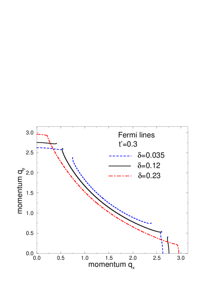
Figure 2: The evolution of the Fermi surface with the opening of the DDW gap.

Second, quite generally, the interband current is present for an electron in a periodic potential, so that the analog of (14) may occur in a multi-band metal as well. The main difference between this case and the discussed DDW state lies in the relative importance of the second inverse mass term in (14). The energy denominator in it involves the interband splitting which is usually large in the multi-band case. The energies of two bands may become closer at the van Hove points in the Brillouin zone, however, the interband current $v_{3}$ vanishes there. These general arguments are inapplicable to the DDW situation as described below.

For the anisotropic dispersion $\xi_{\bf k}$ and DDW order parameter $\Delta_{\bf k}$ the second mass term in Eq.(14) is important. Indeed, the DDW-induced changes in the Hall conductivity are mostly determined by the vicinity of the ”hot spots” in ${\bf k}-$space where $\xi_{{\bf k}}\simeq\xi_{{\bf k}+{\bf Q}}\simeq 0$. Expanding the spectrum around one of these spots we write $\xi_{+}\simeq V_{1}k_{1}$, $\xi_{-}\simeq V_{2}k_{2}$, and $\Delta_{{\bf k}}\simeq\Delta_{hs}+V_{d}k_{1}$. Here $k_{1,2}=k_{x}\pm k_{y}$ and $|\Delta_{hs}|\sim|V_{d}|\ll|V_{1}|\sim|V_{2}|$. These expressions lead to $v_{3}\sim V_{2}$ and a parametrically small energy denominator $\varepsilon_{1{\bf k}}-\varepsilon_{2{\bf k}}\sim|\Delta|$ in (14). Eq.(14) shows then an anomalously large contribution $\sim V_{1}^{2}V_{2}^{2}/|\Delta|$ in the hot spot’s vicinity, $\delta k\sim|\Delta_{0}|/V_{2}$. Observing that ${\cal D}^{\alpha}{\cal D}^{\beta}\hat{h}$ in (9) is finite near the hot spots, one expects that the second mass term enhances substantially the anomalous contribution from the first term in (14). The resulting change in the Hall conductivity, $\delta\sigma_{xyz}$, is estimated as

$$\delta\sigma_{xyz} \simeq e^{3}\tau^{2}2\pi^{-1}V_{2}V_{d}sign(V_{1}\Delta_{hs}).$$ (15)

We see that $\delta\sigma_{xyz}$ is negative for the above form of the spectrum, thus enhancing the absolute value of the (negative) $\sigma_{xyz}$.

We emphasize that the correction Eq.(15) which is linear in $|\Delta_{0}|$ explicitly contains the gap velocity $V_{d}$. In the case of an s-wave order parameter, $\Delta_{\bf k}=\Delta_{0}=constant$, the velocity $V_{d}=0$ and the first nonvanishing correction to $\delta\sigma_{xyz}$ would be of order of $\Delta_{0}^{2}$ and thus much smaller.

Figure 3: The zero-temperature results for the doping dependence of the conductivity $\sigma$ and the Hall conductivity $\sigma_{H}$ divided by $e^{2}\tau$ and $e^{3}\tau^{2}$, respectively. The contributions from the first and second inverse mass term in (14) to $\sigma_{H}$ are shown as $\sigma_{H}^{(1)}$ and $\sigma_{H}^{(2)}$, respectively.

Figure 4: The temperature dependence of the Hall number $n_{H}=-\sigma^{2}/\sigma_{H}$.

We have performed numerical calculations for $\sigma_{xx}=\sigma$ and $\sigma_{xyz}=\sigma_{H}$ using Eqs.(10) and (14) and our Hamiltonian Eq.(1). In rough agreement with the large-N limit of the $t-J$ modelCappelluti we modelled the gap by $\Delta_{0}=\bar{\Delta}(T)\sqrt{(}1+\mu)\Theta(1+\mu)$, where $\mu$ is the chemical potential, $\bar{\Delta}(0)=0.58$, a BCS temperature dependence is assumed for $\bar{\Delta}(T)$, and $t$ is used as the energy unit. The onset of the gap at $\mu=-1$ corresponds to the critical doping $\delta_{c}\sim 0.145$ at $T=0$ and to the critical temperature $T_{c}\sim 0.064$ at $\delta=0.075$, using always $t^{\prime}=0.3$. Fig. 2 shows Fermi lines of this model for three different dopings. The Fermi lines consist of arcs around the nodal direction and lines near the antinodal points. Lines for the same doping end at the boundary of the magnetic Brillouin zone at different points because of the presence of the gap.

The conductivities at zero temperature were obtained as integrals over Fermi lines. We used several hundred points to parametrize the Fermi lines ensuring that similar grids were used for different lines to achieve a numerical cancellation of singular terms. The temperature dependent conductivities $\sigma(\mu,T)$ were calculated using

$$\sigma(\mu,T)=\int dx\,\frac{\partial n(x)}{\partial x}\sigma(\mu+x,0)=\int_{0}^{1}dn\,\sigma(\mu+x(n),0),$$

with $x(n)=T\ln(n^{-1}-1)$. The latter redefinition of the integration regularizes the calculation at low temperatures.

The conductivity $\sigma$ has a contribution linear in the order parameter coming from the vicinity of hot spots, $\delta\sigma_{xx}\simeq-e^{2}\tau\pi^{-1}|V_{2}\Delta_{hs}/V_{1}|$. It translates to a square root dip near the critical values $\delta_{c}$ and $T_{c}$, as can be seen in the curve for $\sigma$ in Fig. 3 for the case of $\delta_{c}$. Assuming that most of the scattering is due to impurities, $\tau$ is qualitatively unchanged at $T_{c}$. Consequently, the square root feature should be observable not only in $\sigma_{H}$ but also in $\sigma$. Note, however, that this dip in $\sigma_{H}$ and $\sigma$ is determined by $\frac{d\Delta_{\bf k}}{d{\bf k}}$ and $\Delta_{\bf k}$ at hot spots, respectively. As shown in Fig. 3 the usual expression for $\sigma_{H}$ (first term in Eq.(14), denoted by $\sigma_{H}^{(1)}$), exhibits only a very weak change at $\delta_{c}$ as a function of doping. In contrast to that, the new term (second term in Eq.(14), denoted by $\sigma_{H}^{(2)}$), shows a well-pronounced square-root behavior near $\delta_{c}$ and dominates the change in the total Hall conductivity $\sigma_{H}=\sigma_{H}^{(1)}+\sigma_{H}^{(2)}$. The temperature dependence of the conductivities is qualitatively similar to the doping one.

Fig. 4 depicts the temperature dependence of the Hall number $n_{H}=-{\sigma}^{2}/\sigma_{H}$. The curve denoted by $n_{H}^{(1)}$ is based on the usual expression, the curve $n_{H}$ on our complete expression including the extra mass term. The onset of the DDW again causes an approximate square root decay below $T_{c}$ in both cases. From a quantitative point of view it is clear from this Figure that the conventional theory gives only roughly 2/3 of the decay so that the discovered new term cannot be neglected in quantiative calculations.

In conclusion, we derived an expression for the Hall conductivity $\sigma_{H}$ in the CDW state including also the interband current contribution. As a result, there is an additional term to $\sigma_{H}$ which may be interpreted as a renormalization of the mass and which is especially important for momentum-dependent CDW order parameters. It is shown numerically that the new term increases the anomalous contribution $\sim\sqrt{T_{c}-T}$ to $\sigma_{H}$ by about a factor 2 in the case of the DDW.

References

• (1) B. Dora, A. Virosztek, and K. Maki, Phys. Rev. B64, 041101 (2001).
• (2) A.H. Castro Neto, Phys. Rev. Lett. 86, 4382 (2001).
• (3) E. Cappelluti and R. Zeyher, Phys. Rev. B59, 6475 (1999).
• (4) S. Chakravarty, R.B. Laughlin, D.K. Morr, and Ch. Nayak, Phys. Rev. B63, 94503 (2001).
• (5) W.Kim, J.-X.Zhu, J.P.Carbotte, C.S.Ting, Phys. Rev. B65, 064502 (2002); W.Kim, J.P.Carbotte, Phys. Rev. B66, 033104 (2002).
• (6) S.Chakravarty, C.Nayak, S.Tewari, X.Yang, Phys. Rev. Lett. 89, 277003 (2002).
• (7) M.R. Norman, Qimiao Si, Ya.B.Bazaliy, R.Ramazashvili, Phys. Rev. Letters 90, 116601 (2003); see also cond-mat/0312168.
• (8) J.M. Ziman, Electrons and Phonons, (Clarendon Press, Oxford, 1960).
• (9) E.M.Lifshitz, L.P.Pitaevskii, Statistical Physics, part 2, vol. 9 of Course of Theoretical Physics, (Butterworth-Heinemann, Oxford, 2002).
• (10) G.D. Mahan, Many-Particle Physics, (Kluwer Academic/Plenum Publishers, New York, 2000).
• (11) B.L.Altshuler, D.Khmel’nitskii, A.I.Larkin, P.A.Lee, Phys. Rev. B22, 5142 (1980).
• (12) H. Ebisawa, H. Fukuyama, Prog. Theor. Phys. 42, 512 (1969).