Fermion kinetics in the Falicov-Kimball limit of the three-band Emery model

Abstract

The three-band Emery model is reduced to a single-particle quantum model of Falicov-Kimball type, by allowing only up-spins to hop, and forbidding double occupation by projection. It is used to study the effects of geometric obstruction on mobile fermions in thermodynamic equilibrium. For low hopping overlap, there appears a plateau in the entropy, due to charge correlations, and related to real-space disorder. For large overlap, the equilibrium thermopower susceptibility remains anomalous, with a sign opposite to the one predicted from the single-particle density of states. The heat capacity and non-Fermi liquid response are discussed in the context of similar results in the literature. All results are obtained by evaluation of an effective single-particle free-energy operator in closed form. The method to obtain this operator is described in detail.

I Introduction

There is at present no paradigmatic ‘non-Fermi liquid’ in more than one dimension, in the same sense as there is the Luttinger liquid in the 1D case. It is therefore of continuous interest to study failures of the Fermi liquid concept in special cases, accessible to concrete calculation. The behavior of electrons in the presence of localized obstructions has long been a fertile ground for investigating deviations from simple Fermi liquid behavior. Examples are the quantum Hall effect von Klitzing (1986), the Kondo problem Andrei et al. (1983), localization by impurities Anderson (1978a), and the Mott metal-to-insulator transition Mott (1968). All of these save the last involve fixed impurity distributions, and their unusual behavior is related to the creation of localized states in the presence of scatterers. Because of this, states accessible to weak probes cannot be understood in the picture of nearly independent quasiparticles.

The Mott transition is unique among the above because the localized obstructions are the mobile electrons themselves, due to the strong on-site repulsion between electrons of the opposite spin. This means translational invariance is not broken, and obstruction is dynamical, which makes the problem much more difficult than with quenched disorder. Despite many contributions which have shaped our present understanding Hubbard (1963); Gutzwiller (1965); Brinkman and Rice (1970); Anderson (1978b); Kotliar and Ruckenstein (1986); Kotliar et al. (1988); Metzner and Vollhardt (1989); Georges et al. (1996), no picture of the Mott transition has emerged to date, which convincingly describes the phenomenon in space and time.

Motivated by the Mott problem in the charge-transfer limit, which is of primary interest for high-temperature superconductors Anderson (1987), the present work describes non-Fermi liquid behavior in one model of the Falicov-Kimball Falicov and Kimball (1969) group, which are intermediate between the quenched-disorder case and the fully dynamical Mott case: the disorder is heavy, but annealed. In this way translational invariance is restored at the level of the ensemble, while the dynamics still relates to static disorder. The present model is the only one in the group in which the disorder is truly geometric, i.e. quantum processes do not physically interact with any classical degree of freedom. This makes it an interesting test-bed for non-Fermi liquid behavior, and indeed it is found that geometric obstruction induces collective behavior in the ‘strange metal’ state beyond half-filling. It somewhat resembles normal ³He at 0.5 K, where the entropy saturates at $\ln 2$ per atom Seiler et al. (1986), simply because the atoms push against each other, obstructing kinetic motion. In the limit of low hopping overlap, the model develops an unexpected similarity to the Kauzmann paradox Kauzmann (1948) in vitreous liquids, despite the fact that all calculations are at equilibrium, so one cannot speak of kinetic slow-down in the usual sense.

For intermediate-to-large overlaps, the model appears at first sight as a renormalized Fermi liquid. However, the ‘equilibrium thermopower,’ $\partial\mu/\partial T$, behaves exactly oppositely to what is predicted from the effective one-particle density of states (1$p$-DOS) at the same temperature and filling. This persistence of quantum collectivity is observed because geometric obstructions take the form of boundary conditions, so they cannot be suppressed by hopping fluctuations.

The technique used to analyze the equilibrium properties of the model is presented here for the first time. It enables one to find a closed analytical expression for the free energy. The essential idea is to remain in the Fock space of the mobile fermions, while evaluating the logarithm of the annealed partition function. The one-particle part of this logarithm is then itself a one-particle operator in Fock space, and can be diagonalized exactly, just like any tight-binding Hamiltonian. With such a careful treatment of Pauli correlations, it is sufficient to expand the annealed free energy to the first non-trivial term in a Kubo cluster cumulant expansion Kubo (1962). The resulting analytical expression is exactly correct in both the atomic and metallic limits, and qualitatively compares well with numerical calculations on similar models.

II The model

II.1 Brief description

Figure 1: The random-tiling model. Black lines are hopping integrals for up-spins, connecting copper (black) and oxygen sites (white). The hopping integrals are turned off where there is a down-spin on a copper site.

The geometric Falicov-Kimball model used here has been introduced previously Sunko and Barišić (1996). It is given by the following modification of the well-known Emery (three-band) model Emery (1987):

$$H=\varepsilon_{d}\sum_{i,\sigma}\hat{n}_{i\sigma}+\varepsilon_{p}\sum_{i,\sigma}(\hat{n}_{x,i\sigma}+\hat{n}_{y,i\sigma})+t\sum_{i}(1-\hat{n}_{i\downarrow})\left(d^{\dagger}_{i\uparrow}P^{\vphantom{\dagger}}_{i\uparrow}+P^{\dagger}_{i\uparrow}d^{\vphantom{\dagger}}_{i\uparrow}\right)\,,$$ (1)

where $P^{\vphantom{\dagger}}_{i\sigma}=p^{\vphantom{\dagger}}_{i-\hat{x}/2,\sigma}+p^{\vphantom{\dagger}}_{i-\hat{y}/2,\sigma}-p^{\vphantom{\dagger}}_{i+\hat{x}/2,\sigma}-p^{\vphantom{\dagger}}_{i+\hat{y}/2,\sigma}$ describes the four oxygen $p$-orbitals around a copper $d$-orbital, and $\hat{n}_{i\sigma}$, $\hat{n}_{x,i\sigma}$, $\hat{n}_{y,i\sigma}$ are the number operators of the copper and oxygen sites. Notice that only up-spins can hop. This is a simple realization of the idea behind Gutzwiller’s approximation: fermions of one spin orientation see those of the other ‘as if occupying a band of width zero’ Gutzwiller (1965). The static down-spins are scattered at random. If one lands on an oxygen site, it pays the price of a charge-transfer energy $\Delta_{pd}=\varepsilon_{p}-\varepsilon_{d}>0$ between oxygen and copper, but is otherwise inactive. Thus the mobile up-spins see a lattice with defects, different for each arrangement of down-spins. The situation is summarized in Figure 1. (For those familiar with the Emery model, note that the up- and down-spins here correspond to physical holes in the copper $d$-orbitals, not electrons.)

In this variant of the Falicov-Kimball Falicov and Kimball (1969) model, there is no physical scattering off the heavy classical spins. Instead the mobile spins see a ‘torn’ lattice with open boundary conditions where the hopping has been turned off. Thus they are in the strong-coupling limit on the one hand, and there is no singularity in their Hamiltonian, on the other. Now there intervenes a significant topological simplification, namely the ‘crosses’ of hopping overlaps impinging on copper sites tile the plane, as visible in Fig. 1. This gives the model its name, random-tiling (RT) model, and makes it possible to express the annealed free energy of the problem by a Kubo cluster-cumulant expansion without leaving the Fock space of up-spins Sunko and Barišić (1996); Sunko . Double occupation of copper sites is disallowed by a separate factor $\exp(-\beta U\sum_{i}\hat{n}_{i\uparrow}\hat{n}_{i\downarrow})$ in the partition function, with $U\gg\Delta_{pd}$. This factor is not entangled with the Hamiltonian, so it is not an interaction, but pure bookkeeping, to force all the mobile spins away from the ‘torn’ part of the lattice. The projector $(1-\hat{n}_{i\downarrow})$ in Eq. (1) is treated exactly, which is essential Millis and Coppersmith (1991): both the Pauli principle and the geometric obstruction are treated on an equal footing. One projects the Fock-space Kubo expansion onto the single-particle subspace, and keeps the first non-trivial term, while higher single-particle terms can be shown to be negligible. This gives a one-particle quantum free-energy operator, whose spectrum can be exactly obtained in closed form. It is built from up-spin wave functions which anneal the geometric disorder. It provides the effective background for all residual (two-particle) interactions, so it is of interest to study by itself. The Mott-Hubbard transition has already been studied in some detail Sunko (2000).

II.2 Detailed derivation

The present section is purely technical, and quite independent of the rest of the article. It describes how the annealed free energy of the random-tiling model can be written without leaving the Fock space of up-spins. The one-particle part of this expression takes the form of a rapidly convergent cluster cumulant expansion around the atomic limit. The main strength of the procedure is that it never violates either the geometric or the Pauli constraints. In particular, it is shown that the same closed expression exactly recovers the metallic free-fermion limit for the up-spins, when the down-spin concentration goes to zero. This is the opposite limit from the atomic one, which attests to the advantage of working in Fock space. Such physical considerations are collected in the last part of this section, to which one may prefer to skip at first reading.

II.2.1 Problem and method

The physical picture described above corresponds at equilibrium to the evaluation of the canonical partition function

$$Z={\mathrm{tr}}\;e^{-\beta H}$$ (2)

where $H$ is the Hamiltonian (1), under the geometric constraint, that mobile up-spins do not land on the copper sites occupied by the down-spins, to which the hopping has been turned off by the projector in (1). As already mentioned above, this is implemented by actually evaluating the unconstrained trace of

$$Z={\mathrm{tr}}\;e^{-\beta H}e^{-\beta V}={\mathrm{tr}}\;e^{-\beta V/2}e^{-\beta H}e^{-\beta V/2},$$ (3)

where the disentangled term $e^{-\beta V}$ enforces the constraint, with

$$V=U\sum_{i}\hat{n}_{i\uparrow}\hat{n}_{i\downarrow}.$$ (4)

(The form with $V/2$ turns out to be more convenient for later manipulation.) It puts the mobile up-spins onto that part of the lattice which is not ‘torn’ by the down-spins on copper sites, acting through the projector $1-\hat{n}_{i\downarrow}$ in Eq. (1). One can easily put $U\to\infty$ in the final expressions, but it is neater to keep a finite $U\gg\Delta_{pd}$. As expected, the results are numerically independent of $U$ in this limit.

The trace over down-spins in Eq. 3 is trivial to perform, and results in rather laborious expressions of the generic form

$$\sum_{\{i_{1},i_{2},\ldots,i_{M}\}\subset{\mathcal{L}}}f(A_{i_{1}}+\ldots+A_{i_{M}})\equiv U_{LM}.$$ (5)

Here $A_{i}$ are site-labelled operators in the Fock space of up-spins, essentially the crosses in Fig. 1. This is obvious, since a given configuration of down-spins corresponds to some choice of $M$ lattice sites where the hopping survives, out of a total $L$ sites ($L$ is volume) comprising the lattice ${\mathcal{L}}$. Note that $f$ is a function of Fock-space operators for the up-spins. It is something like

$$f(X)\sim\exp\left[-\beta(H_{0}+X)\right],$$ (6)

where $H_{0}$ is the site Hamiltonian. The $U_{LM}$ are the thermal evolution operators for the annealed disorder with $M$ hopping crosses present. The main point of the method used here is to reorganize expressions like (5) by a combinatorial inversion which is valid for arbitrary non-commuting operators. This allows one to extract the one-particle part of the free energy expansion exactly, and show that corrections to its first (one-site) term are controlled in the range of fillings of interest here.

Physically, the method boils down to a combinatorial interpretation of Kubo’s cluster cumulant formula for the free energy. This is explained at length in Ref. Sunko , where these ideas are used to cover familiar ground. In particular, the reader is reminded that the expansion parameter, corresponding to the concentration in the classical virial expansion, is an occupation probability in the general case Kubo (1962). In the present work, one implements Kubo’s formalism by first performing the combinatorial inversion at the level of the stochastic evolution operators (5), and taking the logarithms only in the last step. To be explicit, introduce the binomial transform

$$U_{LM} = \sum_{p}\binom{L-p}{M-p}U_{L}(p),$$ (7a)

$$U_{L}(p) = \sum_{M}(-1)^{p-M}\binom{L-M}{p-M}U_{LM}.$$ (7b)

When one of these expressions is inserted into the other, the result is an identity, so they are valid independently of what the $U_{LM}$ may be. Then a very short exercise shows that the generating function for the $U_{LM}$’s may be expressed in terms of the $U_{L}(p)$ as

$$\sum_{M}x^{M}U_{LM}=(1+x)^{L}\sum_{p}y^{p}U_{L}(p),$$ (8)

where $y=x/(1+x)$, $0<y<1$. This result depends only on the relation (7a), and in particular, nothing is assumed about commutativity. Since the $U_{LM}$ are canonical evolution operators, the sum in (8) is the corresponding grand canonical operator. Hence $x$ involves the chemical potential for the hopping crosses, $x=\exp(\beta\nu^{\prime})$, say. In the present context, it will be more convenient to express the expansion parameter $y$ in terms of the chemical potential of the static down-spins, call it $\nu$. Since the hopping cross is absent when the down spin is present on a copper site, the two chemical potentials are effectively connected by a particle-hole transformation. When the energy origin is conveniently chosen so that $\varepsilon_{d}=0$, this amounts to $\nu=-\nu^{\prime}$, i.e.

$$y=\frac{1}{1+e^{\beta\nu}}.$$ (9)

For the range of concentrations considered in this article, half-filling and beyond, the chemical potential of the static down-spins will turn out to be at the oxygen energy, $\nu\approx\varepsilon_{p}>0$, so that $y$ is exponentially small. Thus it provides rapid convergence in the expansion of the one-particle part of Eq. (3) for these concentrations.

II.2.2 Main expressions

Set the bare copper energy $\varepsilon_{d}=0$. In Emery-model jargon, the ‘hole picture’ is assumed, so $\varepsilon_{p}>\varepsilon_{d}=0$, and as mentioned above, $U\gg\varepsilon_{p}$. Call

$$\widehat{N}_{d\uparrow}=\sum_{i=1}^{L}n_{i\uparrow}$$ (10)

the number operator on the copper sites, which appears in (1). The actual forms encountered in tracing (3) are slightly more complicated than suggested in the previous section, because of the side factors with $V/2$, and because the down spins can also land on the oxygen sites. Overcoming these complications by ordinary diligence, the $U_{L}(p)$, required in (8), are given by

$$U_{L}(0) = e^{-\beta\left(\varepsilon_{p}\widehat{N}_{p\uparrow}+U\widehat{N}_{d\uparrow}\right)},$$ (11)

$$U_{L}(1) = \sum_{i=1}^{L}\left(e^{-\beta(U/2)(\widehat{N}_{d\uparrow}-n_{i\uparrow})}e^{-\beta[\varepsilon_{p}\widehat{N}_{p\uparrow}+t(d^{\dagger}_{i\uparrow}P^{\vphantom{\dagger}}_{i\uparrow}+P^{\dagger}_{i\uparrow}d^{\vphantom{\dagger}}_{i\uparrow})]}e^{-\beta(U/2)(\widehat{N}_{d\uparrow}-n_{i\uparrow})}-U_{L}(0)\right).$$ (12)

Here, $\widehat{N}_{p\uparrow}$ is the number operator on the oxygen sites. Stopping at first order in $y$ in the general expansion (8), the operator to be traced over the up-spins now appears as

$$\sum_{M_{\downarrow}}\binom{qL}{N_{\downarrow}-M_{\downarrow}}e^{-\beta\varepsilon_{p}(N_{\downarrow}-M_{\downarrow})}$$ (13)

$$\times\left[\left[x^{L-M_{\downarrow}}\right]\right](1+x)^{L}\exp\left\{\left[\ln\left(U_{L}(0)+yU_{L}(1)\right)\right]_{1p}\right\},$$

where the notation ‘$[[x^{r}]]\ldots$’ means ‘coefficient of $x^{r}$ in $\ldots$’, and ‘$1p$’ means ‘one-particle part.’ Here $N_{\downarrow}$ is the total number of static down-spins, and $M_{\downarrow}$ is the number of down-spins which have landed on the coppers. The number of oxygen sites per unit cell is $q=2$. In the next section, the logarithm of Eq. (13) will be explicitly computed in Fock space. Assume for now that this has been done, and that the one-particle operator in braces in (13) has been diagonalized. Then the trace can also be performed in the space of up-spins. Introducing a chemical potential $\mu$ for these latter, the trace now reads

$$\sum_{M_{\downarrow}}\binom{qL}{N_{\downarrow}-M_{\downarrow}}e^{-\beta\varepsilon_{p}(N_{\downarrow}-M_{\downarrow})}\frac{(1+e^{-\beta\nu})^{L}Z(\mu,\nu)}{e^{\beta\mu N_{\uparrow}}e^{-\beta\nu(L-M_{\downarrow})}},$$ (14)

where $x$ has been called $e^{-\beta\nu}$, $\nu$ is the chemical potential of the down-spins, and

$$Z(\mu,\nu)=\prod_{k,\alpha}\left(1+e^{\beta(\mu-\varepsilon_{\alpha}(k,\nu))}\right)$$ (15)

is the grand partition function in up-spin space, with $\varepsilon_{\alpha}(k,\nu)$ the energies of the up-spin normal modes, indexed with a band index $\alpha$, and depending on the chemical potential of the down-spins, $\nu$, as well as on a wave vector, $k$. Finally, the sum in (14) is evaluated by taking its largest term, resulting in the following model: find the extremum of

$$\sqrt[L]{Z_{\mathrm{eff}}(\mu,\nu)}=\frac{(1+e^{\beta\nu})(1+e^{\beta(\nu-\varepsilon_{p})})^{q}\sqrt[L]{Z(\mu,\nu)}}{e^{\beta\mu n_{\uparrow}}e^{\beta\nu n_{\downarrow}}},$$ (16)

in the space of $\mu$ and $\nu$, for given concentrations $n_{\uparrow}$ and $n_{\downarrow}$. The extremal equations are

$$n_{\uparrow} = \frac{1}{L}\frac{\partial\ln Z(\mu,\nu)}{\beta\partial\mu},$$ (17a)

$$n_{\downarrow} = \frac{e^{\beta\nu}}{1+e^{\beta\nu}}+q\frac{e^{\beta(\nu-\varepsilon_{p})}}{1+e^{\beta(\nu-\varepsilon_{p})}}+\frac{1}{L}\frac{\partial\ln Z(\mu,\nu)}{\beta\partial\nu}.$$ (17b)

Eq. (17b) is physically transparent: there are static down-spins, sitting in one level at $\varepsilon_{d}=0$, and $q=2$ levels at the oxygen energy $\varepsilon_{p}$. The last term, affecting the count of down-spins, comes from the interaction with the up-spins, as coded by the dependence of their dispersion on $\nu$. This dispersion is derived in the next section, giving a complete, closed model. Its dependence on the chemical potential of the down-spins is expected on general thermodynamic grounds, since the presence of down-spins affects the configurations available to up-spins.

II.2.3 Extraction of the one-particle part

In the previous section, the binomial transform was used to treat the stochastic evolution operator induced by the geometric constraint (annealment). The manipulations were mostly an exercise in bookkeeping. In this section, the Pauli constraint is considered, and the main tool is the evaluation of analytic functions of matrix arguments. This is the straightforward way to evaluate analytic functions of Fock space operators, if one is only interested in the resulting one-particle part. Analytic functions of matrix arguments are evaluated as usual, by diagonalization:

$$F(A)=F(SS^{-1}ASS^{-1})=SF(S^{-1}AS)S^{-1}.$$

To prepare the ground requires, however, one last combinatorial trick. Namely, take the $f(X)$ in (5) to be $\ln(U_{L}(0)+yX)$. Then $\ln(U_{L}(0)+yU_{L}(1))$ can play the role of an ‘$U_{LL}$’ in (5), since $U_{L}(1)$ in (12) is a sum over all site-indexed terms, each playing the role of an ‘$A_{i}$’ in (5). The expansion (7a) with $M=L$ then gives, for this case,

$$\ln\left(U_{L}(0)+y\sum_{i=1}^{L}B_{i}\right)=-\beta(\varepsilon_{p}\widehat{N}_{p\uparrow}+U\widehat{N}_{d\uparrow})$$ (18)

$$+\sum_{i=1}^{L}\left\{\ln\left[U_{L}(0)+yB_{i}\right]-\ln\left[U_{L}(0)\right]\right\}+\sum_{i<j}^{L}\ldots,$$

where the sum over $i<j$ is already a second-order term. Here $B_{i}$ denotes the $i$-th term under the sum in (12). The effective free energy is then

$$F_{\mathrm{eff}}=\varepsilon_{p}\widehat{N}_{p\uparrow}+U\widehat{N}_{d\uparrow}-\frac{1}{\beta}\sum_{i=1}^{L}\left\{\ldots\right\}_{1p},$$ (19)

where the braces refer to the same expression as in Eq. (18). Higher order terms are dropped, because they correspond to higher powers in $y$.

From now on the way is clear, provided one has an algebraic manipulation program. The effective free energy (19) may be rewritten

$$F_{\mathrm{eff}} = \sum_{i}\left.\ln\left(1+V_{i}^{\dagger}\left[U_{0}+y(U_{1}-U_{0})\right]V_{i}\right)\right|_{1p}$$ (20)

$$-V_{i}^{\dagger}{\mathrm{diag}}(\varepsilon_{p}/2,\varepsilon_{p}/2,0,\varepsilon_{p}/2,\varepsilon_{p}/2)V_{i},$$

where $V_{i}={\mathrm{col}}(p^{\vphantom{\dagger}}_{i-\hat{x}/2,\uparrow},p^{\vphantom{\dagger}}_{i+\hat{y}/2,\uparrow},d^{\vphantom{\dagger}}_{i\uparrow},p^{\vphantom{\dagger}}_{i-\hat{y}/2,\uparrow},p^{\vphantom{\dagger}}_{i+\hat{x}/2,\uparrow})$ is the column of Fock-space operators, referring to atoms centered on the $i$-th site, with $d^{\vphantom{\dagger}}_{i\sigma}$ the copper operator. Explicitly, $U_{0}={\mathrm{diag}}(e^{-\beta\varepsilon_{p}}-1,e^{-\beta\varepsilon_{p}}-1,e^{-\beta U}-1,e^{-\beta\varepsilon_{p}}-1,e^{-\beta\varepsilon_{p}}-1)$, and

$$U_{1}-U_{0}=\left(\begin{array}[]{ccccc}\tau_{2}&-\tau_{2}&\tau_{1}&\tau_{2}&-\tau_{2}\\ -\tau_{2}&\tau_{2}&-\tau_{1}&-\tau_{2}&\tau_{2}\\ \tau_{1}&-\tau_{1}&\tau_{0}&\tau_{1}&-\tau_{1}\\ \tau_{2}&-\tau_{2}&\tau_{1}&\tau_{2}&-\tau_{2}\\ -\tau_{2}&\tau_{2}&-\tau_{1}&-\tau_{2}&\tau_{2}\\ \end{array}\right),$$ (21)

with

$$\tau_{0} = w\cos^{2}\frac{\varphi}{2}+\frac{p}{w}\sin^{2}\frac{\varphi}{2}-c,$$ (22a)

$$4\tau_{1} = -w\sin\varphi+\frac{p}{w}\sin\varphi,$$ (22b)

$$4\tau_{2} = w\sin^{2}\frac{\varphi}{2}+\frac{p}{w}\cos^{2}\frac{\varphi}{2}-p,$$ (22c)

where the following shorthand has been used:

$$w=e^{\beta\widetilde{\Delta}_{pd}},\;p=e^{-\beta\varepsilon_{p}},\;c=e^{-\beta U},$$ (23a)

and

$$\sin\varphi = \frac{2t}{\sqrt{\left(\frac{\varepsilon_{p}}{2}\right)^{2}+4t^{2}}},$$ (23b)

$$\cos\varphi = \frac{\varepsilon_{p}/2}{\sqrt{\left(\frac{\varepsilon_{p}}{2}\right)^{2}+4t^{2}}},$$ (23c)

while the exponent in $$w$$ is

$$\widetilde{\Delta}_{pd}=\sqrt{\left(\frac{\varepsilon_{p}}{2}\right)^{2}+4t^{2}}-\frac{\varepsilon_{p}}{2}.$$ (23d)

Coming back to $F_{\mathrm{eff}}$, the one-particle part of the logarithm may be written explicitly, giving

$$F_{\mathrm{eff}}=\sum_{i=1}^{L}V_{i}^{\dagger}TV_{i},$$ (24a)

where

$$T=\left(\begin{array}[]{ccccc}\frac{\varepsilon_{p}}{2}+t_{pp}&-t_{pp}&t_{pd}&t_{pp}&-t_{pp}\\ -t_{pp}&\frac{\varepsilon_{p}}{2}+t_{pp}&-t_{pd}&-t_{pp}&t_{pp}\\ t_{pd}&-t_{pd}&\Delta\varepsilon_{d}&t_{pd}&-t_{pd}\\ t_{pp}&-t_{pp}&t_{pd}&\frac{\varepsilon_{p}}{2}+t_{pp}&-t_{pp}\\ -t_{pp}&t_{pp}&-t_{pd}&-t_{pp}&\frac{\varepsilon_{p}}{2}+t_{pp}\\ \end{array}\right).$$ (24b)

Before the expressions for the matrix elements of $T$ are given, note that (24) is like a simple tight-binding Hamiltonian, which may be diagonalized by a Fourier transform. The spectrum consists of three bands, one of which is nonbonding:

$$\varepsilon_{\pm}(\gamma_{k}^{2}) = \frac{\varepsilon_{p}+\Delta\varepsilon_{d}}{2}+2t_{pp}\gamma_{k}^{2}$$ (25a)

$$\pm\;\sqrt{\left(\frac{\varepsilon_{p}-\Delta\varepsilon_{d}}{2}+2t_{pp}\gamma_{k}^{2}\right)^{2}+4t_{pd}^{2}\gamma_{k}^{2}},$$

$$\varepsilon_{0} = \varepsilon_{p},$$ (25b)

with $\gamma_{k}^{2}=\sin^{2}k_{x}/2+\sin^{2}k_{y}/2$. The dispersion (25) is the effective spectrum of up-spins in the presence of static down-spins. It was denoted, schematically, as $\varepsilon_{\alpha}(k,\nu)$ in the definition (15) of $Z(\mu,\nu)$.

In order to specify the model (16) in full, it only remains to write down the matrix elements of $T$ in (24). Define $\zeta_{\pm}$ by

$$e^{-\beta\zeta_{\pm}} \equiv \frac{p+c}{2}+y\left(2\tau_{2}+\frac{\tau_{0}}{2}\right)$$ (26)

$$\pm\;\sqrt{\left[\frac{p-c}{2}+y\left(2\tau_{2}-\frac{\tau_{0}}{2}\right)\right]^{2}+4y^{2}\tau_{1}^{2}},$$

where $y=1/(1+e^{\beta\nu})$, and the rest of the notation is as in (22,23), while $\nu$ is, as always, the chemical potential of the static down-spins. Then

$$t_{pd} = \frac{\zeta_{+}-\zeta_{-}}{4}\sin\psi,$$ (27a)

$$4t_{pp} = \frac{\zeta_{+}+\zeta_{-}}{2}+\frac{\zeta_{+}-\zeta_{-}}{2}\cos\psi-\varepsilon_{p},$$ (27b)

$$\Delta\varepsilon_{d} = \frac{\zeta_{+}+\zeta_{-}}{2}-\frac{\zeta_{+}-\zeta_{-}}{2}\cos\psi,$$ (27c)

where

$$\sin\psi = \frac{2y\tau_{1}}{\sqrt{\left[\frac{p-c}{2}+y\left(2\tau_{2}-\frac{\tau_{0}}{2}\right)\right]^{2}+4y^{2}\tau_{1}^{2}}},$$

$$\cos\psi = \frac{\left[\frac{p-c}{2}+y\left(2\tau_{2}-\frac{\tau_{0}}{2}\right)\right]}{\sqrt{\left[\frac{p-c}{2}+y\left(2\tau_{2}-\frac{\tau_{0}}{2}\right)\right]^{2}+4y^{2}\tau_{1}^{2}}}.$$

This completes the derivation of the effective spectrum (25) of the model (16).

II.2.4 Physical considerations

Let us first summarize the physical truncations made in the preceding derivation. Two distinct meanings of ‘first non-trivial term’ were employed. One is to keep to the one-particle part of the Fock space. This is guaranteed by the Fock-space formalism itself, or more technically by the fact that one has passed from operators to numbers only in the last step of the calculation, when diagonalizing the operator (24). The other is to keep to first order in the expansion in $y$. This is a little more tricky, because the final spectrum (25) of the free energy is non-linear in $y$. Here ‘first-order’ actually means first-order at the level of the evolution operator. This is especially evident in the forms (19) and (20). Operationally, the rule is to keep to first order in $y$ under the logarithm, but the one-particle part of the resulting logarithmic operator must be extracted exactly, i.e. without further truncation in $y$.

The above one-particle effective free energy is formally the first (one-site) non-trivial term in an expansion around the atomic limit. In terms of the expansion parameter $y=1/(1+e^{\beta\nu})$, where $\nu$ is the chemical potential of the down-spins, this is an expansion around $y=0$, when the copper sites are completely occupied by down-spins. It will now be shown that the result is correct also for $y=1$, which means no down-spins at all ($\nu\to-\infty$). Then the exact non-interacting band is recovered. This is a very useful check that the two truncation prescriptions discussed in the previous paragraph are mutually consistent. In particular, it shows that keeping to first order in $y$ does not violate the Pauli principle. This is a benefit of working in Fock space — in similar expansions around the classical limit, the Pauli correlations are only taken into account in an inclusion-exclusion procedure Zhi He and Cremer (1991), which remains approximate to all finite orders in the expansion parameter.

Taking $\nu\to-\infty$ in Eq. (26), one gets

$$e^{-\beta\zeta_{+}}\to w, e^{-\beta\zeta_{-}}\to p/w,$$

$$\cos\psi\to-\cos\varphi, \sin\psi\to-\sin\varphi.$$ (28)

Putting all this together, the hopping amplitudes (27) become

$$t_{pd}\to t,\;t_{pp}\to 0,\;\Delta\varepsilon_{d}\to 0,$$

which gives the dispersion for the free limit of the Hamiltonian (1). This confirms that the one-particle part of the original problem has been treated correctly. It is also easy to verify that putting $y=0$ gives the same result as $t=0$ in the original Hamiltonian, but this is of course expected.

It will now be shown that the one-particle part of the expansion in $y$ is controlled, for the concentrations considered in this article. The higher order terms in $y$ contain one-particle contributions coming from the diagonalization of larger ‘molecules,’ such as Cu₂O₇ (say), which appears when two ‘hopping crosses’ share an oxygen. This has the typical structure of a connected-cluster expansion. The general term is $y^{p}U_{L}(p)$. For down-spin concentrations beyond half-filling, the saddle-point equations give $\nu\approx\varepsilon_{p}$, i.e. $y\sim e^{-\beta\varepsilon_{p}}=e^{-\beta\Delta_{pd}}$ (remember we put $\varepsilon_{d}=0$). Note from Eqs. (20) and (23) that the magnitude of the term multiplying $y$ is roughly $w=e^{+\beta\widetilde{\Delta}_{pd}}$, so the overall estimate for the first term is $yU_{L}(1)\sim yw\sim e^{-\beta(\Delta_{pd}-\widetilde{\Delta}_{pd})}<1$. Physically, $\widetilde{\Delta}_{pd}$ is just the hybridization energy associated with the diagonalization of a single CuO₄ ‘molecule.’ A larger cluster will have a larger hybridization gain, but it will also be suppressed by a larger power of $y$. Since hybridization gains quickly saturate as a function of cluster size, they cannot offset the addition of a whole bare $\Delta_{pd}$ with each new Cu site added to a ‘molecule.’ Hence the expansion is rapidly convergent in the range of fillings considered below.

For down-spin fillings below the Mott transition, i.e. corresponding to the lower Hubbard band (LHB), $\nu\approx\varepsilon_{d}=0$, meaning $y$ is some appreciable fraction of unity, not exponentially small. Then presumably higher-order single-particle terms could play a role. This is consistent with the fact that in the LHB, there is a significant contribution of the interaction to the entropy, while the same is exponentially small beyond the Mott transition — the system goes from liquid to gas, absorbing latent heat Sunko and Barišić (1996); Sunko (2000). Nevertheless, the fact that the exact band result is recovered in the limit $y=1$ suggests that the present calculation should not be qualitatively incorrect even in the LHB, not of main interest here.

III Results

III.1 Small hopping overlap

In the model, the entropy of mobile spins is formally given by the usual single-particle expression

$$S_{\uparrow}=-\int_{BZ}\left[f_{\mu}(\varepsilon_{-})\ln(f_{\mu}(\varepsilon_{-}))+(1-f_{\mu}(\varepsilon_{-}))\ln(1-f_{\mu}(\varepsilon_{-}))\right],$$ (29)

where $\mu$ is the chemical potential of the mobile spins, while the effective bonding band $\varepsilon_{-}$, given by Eq. (25), is a function of $\nu$, the chemical potential of the static spins, and of the temperature. Both $\mu$ and $\nu$ change with temperature, since the particle number is fixed for the up- and down-spins separately. In Fig. 2, the entropy of mobile spins is shown as a function of temperature, for two values of the bare hopping and several concentrations. The most striking feature of the figure are broad plateaus, or inflections, indicating dips of width $\sim$ 100 K in the heat capacity $c_{V}$ of the system. The curve at $n=1.8$ even shows a ‘Kauzmann paradox’ Kauzmann (1948), where extrapolation of the high-energy part would give a negative entropy at zero temperature. Of course, the entropy is strictly zero at $T=0$, since the free energy (16) is microscopic by construction. The plateaus correspond to regions of low $c_{V}$, associated with the difficulty of finding new states, which gives peaks in $c_{V}$ (not shown) between $T=0$ and the plateau positions.

Figure 2: Entropy of mobile spins (29), for $t=0.25$ eV (left three curves), and $t=0.5$ eV (right four curves). Curves are marked by the corresponding concentration. Saturation plateaus are clearly visible. Here $\Delta_{pd}=3$ eV, $U=10$ eV, and $n=2n_{\uparrow}=2n_{\downarrow}$.

Figure 3: Comparison of $S_{\uparrow}(T)$ (thick line) and $S_{\uparrow,{\mathrm{C}u}}(T)$, Eq. (30) (thin line), for $t=0.31$ eV, $n=1.2$, and other parameters as in Fig. 2.

The plateaus are identified with static disorder in the obstructed copper sites. The proof is as follows: call the concentration of up-spins on the coppers $m_{\uparrow}$. If they were static, their contribution to the entropy would be just

$$S_{\uparrow,{\mathrm{C}u}}=-m_{\uparrow}\ln(m_{\uparrow})-(1-m_{\uparrow})\ln(1-m_{\uparrow}),$$ (30)

and beyond half-filling, each copper site would be singly occupied, either by an up-spin or a down-spin. Thus $m_{\uparrow}=1-m_{\downarrow}$, in the static case, where $m_{\downarrow}$ is the concentration of down-spins on the coppers. Since $m_{\downarrow}$ is easily obtained from the calculation, one can use it to construct $S_{\uparrow,{\mathrm{C}u}}(T)$ from Eq. (30), and compare these values with the actual $S_{\uparrow}(T)$ from the same calculation, given by Eq. (29). As shown in Fig. 3, the hypothetical static entropy (30) coincides with the calculated entropy at the inflection point, beyond which the latter begins to rise. To show this more clearly, the hopping overlap is slightly increased in this figure, so the plateau is not quite flat.

Figure 4: Chemical potential of mobile spins (thick line) corresponding to $S_{\uparrow}(T)$ in Fig. 3. The bottom and top of the effective band are given by thin and dashed lines, respectively.

This means that in the regime $t\ll\Delta_{pd}$, excitation of the system proceeds in two steps. First the copper positional degrees of freedom are fully saturated: their entropy cannot be greater than that of the correspondig static disorder. Then the translational ones, involving the oxygens, are activated, but only after a small ($\sim$ 100 K) region is crossed, where there are no new states. The two steps are better separated when the bare hopping is smaller: note the difference between the curves for $t=0.25$ eV and $t=0.5$ eV in Fig. 2.

Figure 4 shows how the model technically achieves this behavior. As usual with single-particle effective models, collectivity enters through the solution of the saddle-point equations, which fix the chemical potential at a given concentration and temperature. The chemical potential traverses the band fairly rapidly as the temperature increases, and leaves it roughly around the temperature at which the plateau appears. As it passes through the region where the 1$p$-DOS drops, there appears a lack of new states for the system. Once in the (Maxwellian) tail of the Fermi distribution, the oxygen degrees of freedom are further excited. In this sense, the system is again analogous to ³He. However, there is no regime of classical kinetic motion in the model, since the bands are built-in by assumption.

III.2 Large hopping overlap

Figure 5: Left column: entropy of mobile spins (29). Right column: equilibrium thermopower (31). Upper row: $n_{\uparrow}=n_{\downarrow}=0.6$. Lower row: $n_{\uparrow}=0.6$, $n_{\downarrow}=0.001$. Lines, thin to thick: hopping $t=0.25,0.5,0.75,1.0$ eV, respectively, with $\Delta_{pd}=3$ eV.

Collective effects persist in the model even when the hopping overlap becomes so large that the effective band appears to be normally metallic, with a well-defined Fermi surface. They are no longer immediately evident at the level of the entropy, but remain in the susceptibility. This is shown in Figure 5. For comparison, the lower row shows the limit of free fermions. The entropy for $n_{\uparrow}=n_{\downarrow}=0.6$ (upper left panel) rapidly begins to look ‘normal’ as the hopping overlap increases (thicker curves).

The right column in the figure shows that this impression is misleading, however. It gives the equilibrium susceptibility, corresponding to the thermopower,

$$S_{eq}=-\frac{1}{e}\frac{\partial\mu}{\partial T}.$$ (31)

In a simple rigid band, $S_{eq}$ should change sign from positive to negative as the filling goes beyond one-half. This is because the chemical potential goes down with the temperature, if the 1$p$-DOS goes up with the filling, and vice versa.

For the free model (lower right panel), the equilibrium thermopower (31) is indeed negative. Now add down-spins until the model undergoes its Mott-Hubbard transition Sunko (2000). Then the up-spin $S_{eq}$ (31) becomes positive, even though the Fermi surface does not change with respect to the free situation. It is physically clear what is happening: the kinetic blocking effects are strongest around half-filling, so going beyond it increases the available degrees of freedom, since the mobile up-spins on the oxygens are not blocked. A similar outcome is expected from the effect of antiferromagnetic (AF) correlations above the transition, however there it would be traced to the appearance of a dip in the single-particle spectrum. Namely, such a 1$p$-DOS has a minimum around half-filling, so that beyond it, it rises again, just like at the bottom of the band. Thus in the spin channel, an anomalous susceptibility is due to a normal Fermi-liquid response. By contrast, in the charge channel and beyond the Mott-Hubbard transition, the response cannot similarly be inferred from the single-particle spectrum. Even though the model (16) is formally single-particle and in the metallic regime, it is not a normal Fermi liquid.

III.3 Heat capacity

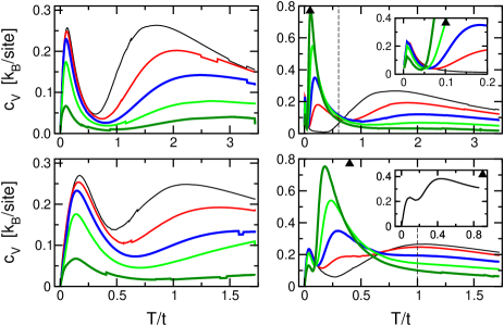
Figure 6: Heat capacities of the random-tiling model. Left (right) column: below (above) half-filling. Thin to thick: left, $n=2n_{\uparrow}=2n_{\downarrow}=0.9,0.7,0.5,0.3,0.1$, right, $n=2n_{\uparrow}=2n_{\downarrow}=1.0,1.2,1.4,1.6,1.8$, respectively. Upper row: $t=0.5$ eV, $\Delta_{pd}=3$ eV. Lower row: $t=1$ eV, $\Delta_{pd}=3$ eV. Vertical dashed line: renormalized charge-transfer scale $\widetilde{\Delta}_{pd}$, Eq.(23d). Insets: upper, detail of the narrow peak; lower, $n=1.4$, $t=2$ eV, $\Delta_{pd}=3$ eV. Black triangles on the axes: $W/t$, Eq. 34.

The heat capacities of the random-tiling model are shown in Fig. 6 (thinner lines are always closer to half-filling). In the LHB (left column), there is a transfer of spectral intensity with doping, between a low- and high-energy scale, both of which already exist at half filling. The latter is still significantly lower than the bare charge-transfer scale $\Delta_{pd}$, which takes the role of $U$ in the present context. This is an effect of hybridization, as mentioned above: the larger the hopping overlap, the lower this ‘high’ scale becomes (note that the horizontal axes in the two rows are different). Below the Mott-Hubbard transition, the equilibrium thermopower is of the same sign as in the free case $n_{\downarrow}\to 0$ (Fig. 5), even for $2n_{\uparrow}=2n_{\downarrow}=0.9$.

Concentrations beyond half-filling cannot be studied in a one-band model. In the present three-band setting, there appears another low-energy peak between the two peaks present at half-filling, which quickly draws strength from the high-energy peak as the doping increases. The new low-energy scale induced by doping is specific to the three-band model in the ‘in-gap’ concentration range. All the relevant scales can be extracted analytically in the limit $T\to 0$, since in that limit the chemical potential of the down spins is forced to one of two known values: $\nu\to\varepsilon_{d}=0$ in the lower Hubbard band (LGB), and $\nu\to\varepsilon_{p}$ in the in-gap band (IGB), beyond the Mott-Hubbard transition. The expressions (27) are easy to evaluate in these limits. Below the transition, the width of the lower Hubbard band is practically unchanged from the non-interacting value

$$W_{0}=\sqrt{\left(\frac{\Delta_{pd}}{2}\right)^{2}+8t^{2}}-\frac{\Delta_{pd}}{2}\;\;\;\mathrm{(LHB)},$$ (32)

where $\Delta_{pd}=\varepsilon_{p}-\varepsilon_{d}$. Here the only effect of strong correlations on the band is a small but finite shift of the copper level downwards,

$$\lim_{T\to 0}\Delta\varepsilon_{d}=\Delta_{pd}\sin^{2}\frac{\varphi}{2}-\widetilde{\Delta}_{pd}\cos^{2}\frac{\varphi}{2}<0\;\;\;\mathrm{(LHB)}.$$ (33)

The IGB is, on the other hand, strongly affected by correlations. The copper level is shifted upwards, and the band is significantly narrowed. Its width in the zero temperature limit is Sunko (2000)

$$\lim_{T\to 0}W=\frac{\widetilde{\Delta}_{pd}}{1+\Delta_{pd}/(2\widetilde{\Delta}_{pd})}\;\;\;\mathrm{(IGB)}.$$ (34)

The copper level shift is now large and positive:

$$\lim_{T\to 0}\Delta\varepsilon_{d}=\Delta_{pd}-\widetilde{\Delta}_{pd}\cos^{2}\frac{\varphi}{2}>0\;\;\;\mathrm{(IGB)}.$$ (35)

Instead of using this formula, it is much more convenient to note that the distance from the bare oxygen position $\varepsilon_{p}$ to the middle of the IGB is just $\widetilde{\Delta}_{pd}$ in the same limit, i.e. the uppper edge of the IGB is given by any of the two formulas

$$\lim_{T\to 0}\left(\varepsilon_{d}+\Delta\varepsilon_{d}\right)=\lim_{T\to 0}\left(\varepsilon_{p}-\widetilde{\Delta}_{pd}+\frac{W}{2}\right)\;\;\;\mathrm{(IGB)}.$$ (36)

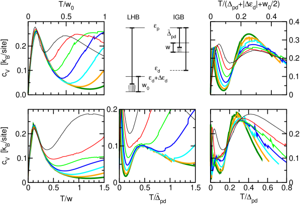
Figure 7: Scales of the peaks in heat capacities for $t=1$ eV. Top (bottom) row: n=0.9 (n=1.1). Lines, thin to thick: $\Delta_{pd}=2,3,4,5,6,7,8$ eV, respectively. The drawing in the middle of the top row schematically shows the scales as barred thick lines, left for the lower Hubbard band (LHB), right for the in-gap band (IGB). The band edges are given by thin horizontal lines, and the occupied levels indicated by shaded squares.

The relevance of these scales for the various peaks is analyzed in Fig. 7. Both below and above the Mott-Hubbard transition, the lowest-energy peak is due to intraband transitions. The peak scales perfectly with $W$ for the IGB, and with $W_{0}$ for the LHB. The high peak in the LHB is due to interband processes, namely excitations into the empty, non-dispersive non-bonding band at $\varepsilon_{p}$, which is a distance $\Delta_{pd}+|\Delta\varepsilon_{d}|+W_{0}/2$ from the Fermi level when the occupied band is nearly half-filled from below. The middle (new) peak in the IGB is also due to interband transitions. As noted above, the middle of this band is a distance $\widetilde{\Delta}_{pd}$ from the oxygen level, giving the scale of the middle peak when the band is nearly half-filled from above.

Finally, the upper (third) peak in the IGB is again due to interband transitions, but of a different kind. They are governed by the bare scale $\Delta_{pd}$, which plays the role analogous to $U$. However, there is no effective band in the model at $\varepsilon_{d}$ beyond the Mott-Hubbard transition (the position $\varepsilon_{d}$ is denoted by a broken line for this reason). The high peak is probing the ‘undressing’ scale, at which the system effectively reverts to the atomic limit. Note that the two thinnest lines, corresponding to $\Delta_{pd}/t=2$ and 3, respectively, do not scale so well by $\Delta_{pd}$ in the right column, and simultaneously have not yet developed a third peak in the middle column. The separation of scales between the middle and high peak should be regarded as a sign of a well-developed charge-transfer regime $\Delta_{pd}>t$ and $n>1$, while for $\Delta_{pd}\approx t$, and $n\approx 1$ from above, the two scales are mixed by hopping fluctuations. The upper peak for these two thin lines has a higher scale than $\Delta_{pd}$, because the copper level they see is still effectively shifted by hopping correlations. This can be corroborated by an amusing ‘quick and dirty’ check (not shown), where one tries to scale the upper peak in the IGB by $\Delta_{pd}+|\Delta\varepsilon_{d}|$, but using the value $|\Delta\varepsilon_{d}|$ for the LHB. Even though this is formally inconsistent, it turns out that the scaling in the lower right panel of Fig. 7 is improved, since the level shift $|\Delta\varepsilon_{d}|$ in the LHB is bigger for stronger hopping fluctuations (smaller $\Delta_{pd}/t$).

The same two IGB regimes, hopping-fluctuation and charge-transfer, may be discerned in the upper and lower panels in the right column of Fig. 6, drawn to absolute scale $t$. In the upper right panel, the input $t/\Delta_{pd}\ll 1$, and the middle (new) peak is higher than $W$ and lower than $\widetilde{\Delta}_{pd}$. Then $\widetilde{\Delta}_{pd}$ appears as a crossover scale between the high-energy peak and the two lower-energy ones. This is the charge-transfer regime, mentioned above.

The hopping-fluctuation regime prevails when the new peak is at low energy with respect to both $W$ and $\widetilde{\Delta}_{pd}$. The lower right panel in Fig. 6 shows the case $\widetilde{\Delta}_{pd}=t$, when some strength still remains in the high-energy peak. The lowest peak has already broadened, leaving no trace of the Brinkman-Rice effect (the scale of the lowest peak has grown to about 1000 K, which is the whole range shown in Fig. 5). The inset shows the hopping-fluctuation regime fully developed, where the upper peak has completely disappeared, so there are again only two peaks like in the LHB (left column). Both are low-energy phenomena ($\widetilde{\Delta}_{pd}/t\approx 1.39$ for the inset). For all of the right column in Fig. 6, the equilibrium thermopower stays of the ‘wrong’ sign, like in the upper row of Fig. 5, no matter how large $t$ is. The fact that the metal is both strange and has an ordinary Fermi surface is consistent with the fact that the unusual two-peaked feature in the heat capacity is observed on a scale smaller than the band-width.

III.4 Comparison with other work

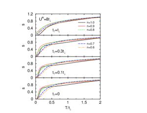
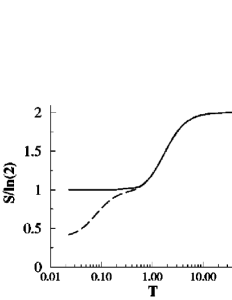
Figure 8: Left: numerical results with the Lanczos algorithm El Shawish et al. (2003). Right: the dynamical cluster approximation Hettler et al. (2000). For a detailed description, see the text.

To compare the present approach meaningfully with others, some general remarks are in order. The approach described here works at present only for the equilibrium properties, a limitation not shared by some other available methods. It is in the thermodynamic limit, like other theoretical schemes, and unlike purely numerical ones. It is unique by being fully analytic. The spectrum (25) is given in closed form, so the only numerical part of the work is to fix the chemical potentials $\mu$ and $\nu$ by Eqs. (17), like in a non-interacting band problem.

One should also have some idea, what such a comparison hopes to achieve. The present paper regards models of Falicov-Kimball type as less interesting for their own sake, than as stand-ins for problems one would really like to treat, the dynamical Mott problem in particular. In this context there is no a priori advantage to one model over another, and it is preferable to concentrate on their similarities. Differences are significant only if they can be settled by a reliable external criterion, such as a known exact result. Hence the purpose of this section is to identify some ‘generic’ behavior of this kind of models, see how the present work fits in, and hopefully understand better the relationship to the Mott type of problem. The papers used for comparison here are selected as representative of recent work, without implication as to merit or priority relative to others.

El Shawish et al. El Shawish et al. (2003) have studied a two-band spinless Falicov-Kimball model, which may be mapped onto a Hubbard model in which the two kinds of spins, up and down, hop with different overlaps, $t_{\uparrow}\neq t_{\downarrow}$. The method was purely numerical, Lanczos algorithm on a lattice of $4\times 4$ sites. The limit $t_{\uparrow}=0$ corresponds to the original model Falicov and Kimball (1969), and their result for this case is shown in the bottom panel on the left in Fig. 8. The full curve for half-filling is directly comparable with the $n=1.0$ curves in Fig. 2. Obviously the general trends are the same, a plateau at $S=\ln 2$, dropping steeply to $S=0$ at $T=0$, and rising very slowly at high temperatures, due to incoherent hopping. However, in Fig. 8 the entropy curves show a gap in the spectrum, while in Fig. 2 there is only a tendency for the effective mass to diverge, or band-width to collapse, like in the Brinkmann-Rice transition, broadened here to a crossover. Recall that the first peak in the heat capacity is scaled by the band-width $W$, which is very small when $t\ll\Delta_{pd}$, meaning the entropy plateau is pulled in to very low temperature instead of being gapped. The gap is missing because only the one-particle part in Fock space is kept; one expects that the two-particle terms would indeed produce a gap near half-filling, once the band-width in the one-particle sector became small enough. (It is interesting that the down-spin entropy in the present model goes to zero at the Mott tranisition Sunko and Barišić (1996), indicating an ordered pattern, even in the absence of two-particle terms.)

The other panels in the left of Fig. 8 show the evolution in $t_{\uparrow}/t_{\downarrow}$, up to the full Hubbard model $t_{\uparrow}=t_{\downarrow}$ in the top panel. The evolution from small $t/\Delta_{pd}$ to large $t/\Delta_{pd}$ in the upper left panel of Fig. 5 is remarkably similar. This could have been expected, because the two spin orientations correspond to the $f$ and $d$ bands in the original two-band spinless Falicov-Kimball model. Hence an equality between the $f$ and $d$ bandwidths is naturally similar to a small (in units of $t$) splitting of the copper and oxygen energies in the present work. The similarity nevertheless raises some issues in relation to the Mott problem, which will be touched upon in the Discussion below.

Hettler et al. Hettler et al. (2000) have studied the two-dimensional one-band Falicov-Kimball model by the dynamical cluster approximation (DCA). This is an extension of dynamical mean-field theory (DMFT Georges et al. (1996)) to clusters of more than one site, embedded in the same, spatially unresolved host medium. In infinite dimensions, the simplest, one-site DCA reduces by construction to the DMFT Georges et al. (1996); Hettler et al. (2000). In finite dimensions, it reduces to the latter’s finite-dimensional analogue, the dynamical mean-field approximation (DMFA). The DCA results Hettler et al. (2000) for the entropy are shown in the right panel of Fig. 8, for a one-site cluster (DMFA, full line), and four-site cluster (broken line). The DMFA retains the full $\ln 2$ per site entropy in the ground state. The four-site DCA does better, but still appears to saturate at about one-half that value near $T=0$. Hence the DCA agrees with the present work, and with the numerical Lanczos results above, in the high-temperature regime, but does not cross over correctly to low temperature.

Figure 9: Heat capacities of the Hubbard model, from Lanczos Bonča and Prelovšek (2003) (left) and quantum Monte Carlo Duffy and Moreo (1997) (right) calculations, discussed in the text. Note that positions of panels with the same concentrations are shifted.

The heat capacities for the IGB in the right column of Fig. 6 cross at two fairly well defined points. Vollhardt Vollhardt (1997) has noted this to be a quite general feature of strongly correlated systems, for families of heat capacity curves parametrized by pressure or concentration in experiment, or the on-site repulsion $U$ in the one-band Hubbard model. The crossing of concentration-parametrized families of curves in the IGB, and their failure to cross in the LHB, fits well with previous observations based on Fig. 5, that it is the IGB, rather than the LHB, which is singularly affected by strong correlations.

A two-peak structure in $c_{V}$ is ubiquitously found in numerical studies of Hubbard-like systems El Shawish et al. (2003); Bonča and Prelovšek (2003); Hettler et al. (2000); Duffy and Moreo (1997). In Fig. 9 on the left are the results of a Lanczos calculation Bonča and Prelovšek (2003) for the one-band Hubbard model on a $4\times 4$ lattice. The right-hand panel is from a quantum Monte Carlo (QMC) calculation on a $6\times 6$ lattice for the same model. They do not cross at any one point, and have two peaks, both of which are generically features of the LHB in the present model. This is not surprising, since concentrations below half-filling are the only ones relevant in the one-band model, because of particle-hole symmetry.

It has been noted Bonča and Prelovšek (2003) that the two calculations in Fig. 9 differ significantly in their outcomes. First, in the QMC results the first peak loses strength much faster with decreasing doping. Second, in the QMC results the peak also moves, while in the Lanczos calculations it stays much in the same place. From the RT model’s point of view, the first peak is expected to scale with the non-interacting bandwidth $W_{0}$, so its position should not depend on concentration, except insofar as due to the changing position of the Fermi level. This is visible in the left column of Fig. 6. The first peak there barely moves, but it moves a little more in the bottom left panel, where the non-interacting band is wider, so the Fermi level shifts more rapidly with concentration. Also, the narrower the LHB, the sharper the first peak, and the more persistent as the concentration decreases. This suggests a physical interpretation of the differences in Fig. 9. The QMC heat capacities imply that the effective band seen by one-band Hubbard electrons below half-filling rapidly widens as the concentration decreases. The Lanczos calculation implies a situation similar to the present model in the LHB: band-width independent of concentration, and the effective band somewhat narrower than the QMC prediction.

To summarize, below half-filling the present analytical method gives similar qualitative behavior of thermodynamic quantities as other, numerically much more involved treatments of one-band models. It is also quantitatively correct in the known exact limits, of high and low temperature, and high and low doping. Where it can be checked quantitatively in the intermediate regime, namely in Fig. 3, it is correct as well. It misses the gap in the up-spin spectrum around half-filling, replacing it with a BR bandwidth collapse, presumably because it retains only one-particle terms in the Fock-space free energy operator. The doping dependence above half-filling is qualitatively different than expected from the one-band analogy. At fixed Hamiltonian parameters, there is a transfer of spectral weight to a new scale, which emerges only with doping. The new scale is connected with interband excitations across the renormalized charge-transfer gap. The present calculation also parallels Lanczos calculations on the Hubbard model, both in the shape and behavior of the peaks in the heat capacity below half-filling.

IV Discussion

The main modelling interest of the present article was to determine when the one-particle construction, adopted to calculate the free energy, indeed corresponds to a Fermi liquid, and when it does not. For that purpose, a minimal negative criterion to observe a non-Fermi liquid at a finite temperature was adopted. A system is not a Fermi liquid if the susceptibilities do not follow from the 1$p$-DOS at that temperature. Put conversely, a necessary condition for a system to be a Fermi liquid is that the 1$p$-DOS responds ‘rigidly’ to an infinitesimal change in temperature.

It has been found previously Sunko (2000) that the Mott transition in the RT model is first order, from a liquid of light particles, in the lower Hubbard band, to a gas of heavy ones, in the renormalized in-gap band. (While the down-spin entropy drops to zero at the transition, indicating AF order, the chemical potential is a monotonous function of the filling, i.e. there is no phase separation.) In the present work, it is shown that while the liquid is a Fermi liquid, the gas is not. The absence of residual interactions (which makes it a gas) has been bought at the price of an anomalous variation of the effective mass with the temperature, such that the thermopower susceptibility (31) cannot be predicted from the 1$p$-DOS at any given temperature. This remains so even if the hopping overlap is large, because the model is always in the strong-coupling limit: changing the hopping does not affect the geometric obstructions, as obvious from Eq. (1). The collectivity involved is very simple. The fermions need to agree which are the best positions for the annealed impurities, in precise analogy to ³He atoms pushing against each other.

At low hopping overlap, this geometric effect so dominates the mean properties of the gas, that it is unable to find new states of motion in a range of temperatures, giving rise to plateaus in the entropy. (Extrapolating experimental trends Seiler et al. (1986), one could imagine similar plateaus appearing in ³He around 0.5 K, if the pressure were sufficiently increased.) These are remarkably similar to Kauzmann plateaus in vitreous liquids, where they are due to the configurational rearrangements falling out of equilibrium. Clearly the Kauzmann phenomenon Kauzmann (1948) is a non-specific sign that kinetic exploration of configuration space has been obstructed, whatever the responsible mechanism. Here it has an interesting connection with the Brinkmann-Rice (BR) bandwidth collapse Brinkman and Rice (1970), which is signalled in Fig. 2 by a steep rise of the entropy from zero temperature at half-filling, indicating an infinite effective mass. By the same token, the entropy plateau means that the effective mass is zero, and it is obtained by continuous deformation of the BR entropy curves with doping. It may seem surprising that obstruction of kinetic motion should be associated with zero thermodynamic effective mass, but note that in the absence of new states, there can be neither conduction nor dissipation. Zero effective mass is just the equilibrium version of what is observed in the Hall effect: the longitudinal Hall conductance and resistance simultaneously drop to (almost) zero at the steps in the transverse resistance, precisely because most of the carriers are localized von Klitzing (1986).

The place of the present calculation among various cluster approaches is simple to state. It is the ordinary Kubo cluster cumulant expansion of the annealed free energy, with the single proviso that it is calculated in Fock space. The transition from operators to numbers is made at the very end, after the single-particle Fock term has been extracted. It is theoretically quite revealing that the results presented here could be obtained by diagonalizing a single CuO₄ molecule, i.e. the lowest non-trivial term in the underlying cluster expansion. Clearly, the main work was in fact done by the algebraic and combinatorial machinery which respectively enforced both the Pauli principle and the geometric constraint. Once these kinematical issues were properly separated from the dynamical ones, it turned out the problem was dominated by the former. This outcome is physically plausible by adiabatic arguments: the low-energy physics of the Falicov-Kimball model is not controlled by any elaborate dynamical correlations, such as one would expect in the Mott case, where the scatterers and the scattered are equally light. It is also consistent with the previous observation Sunko (2000) that the system is a gas beyond half-filling. In the lower Hubbard band, where it is a liquid, higher-order clusters should affect the results, but that is not expected to be qualitatively significant.

The comparison with other, numerically much heavier calculations in the preceding section gives some grounds for reflection on the Mott problem. This has been dominated for the past forty years by Gutzwiller’s intuitions Gutzwiller (1965), that electrons of one spin see those of the other as a ‘smeared background’ (Gutzwiller ansatz), and further ‘as if occupying a band of width zero’ (Gutzwiller approximation). This point of view clearly implies there should be some similarity between Falicov-Kimball and Hubbard-model low-energy behavior. Such a similarity appears to have been found in one of the calculations cited above El Shawish et al. (2003), in the smooth evolution of the entropy as $t_{\uparrow}/t_{\downarrow}$ was raised from zero to one. If one knew that Gutzwiller’s proposals were correct, the very similar evolution of the entropy, observed in the present calculation as $t/\Delta_{pd}$ was increased, would be naturally expected. As things stand, one should keep in mind the alternative resonating-valence-bond (RVB) scenario of Anderson Anderson (1987), in which quantum coherence between the two spin orientations is an essential ingredient of Mott’s insulating ground state. Thus the possibility remains open, that the Falicov-Kimball limit acts as a kind of trap for all approximate treatments of the Hubbard model which incidentally destroy this coherence, over time or space.

It is also of some interest that the heat capacities in the RT model are qualitatively more similar to numerical Hubbard model results, than to one-band Falicov-Kimball results. It is possible that the oxygen degree of freedom plays a role analogous to the ‘other’ spin in the one-band Hubbard model.

To conclude, geometric obstruction in thermodynamic equilibrium has been explored in an analytic single-particle quantum model of Falicov-Kimball type. In the regime $t\ll\Delta_{pd}$, it gives rise to a plateau in the entropy of mobile spins. For $t\sim\Delta_{pd}$, the mobile spins appear to be normally metallic, only with renormalized parameters. Beyond half-filling, their equilibrium thermopower susceptibility nevertheless reflects the microscopic kinematic restrictions, behaving oppositely to what is expected from the single-particle properties. For these fillings, correlation effects in the model do not simplify in the limit of low temperature and large hopping overlap.

V Acknowledgements

Conversations with S. Barišić and E. Tutiš, and one with T.M. Rice, are gratefully acknowledged. Thanks are due to J. Bonča for providing the left panels of Figs. 8 and 9. This work was supported by the Croatian Government under Project 0119256.

References

- von Klitzing (1986) K. von Klitzing, Rev. Mod. Phys. 58, 519 (1986).
- Andrei et al. (1983) N. Andrei, K. Furuya, and J. H. Lowenstein, Rev. Mod. Phys. 55, 331 (1983).
- Anderson (1978a) P. W. Anderson, Rev. Mod. Phys. 50, 191 (1978a).
- Mott (1968) N. F. Mott, Rev. Mod. Phys. 40, 677 (1968).
- Hubbard (1963) J. Hubbard, Proc. R. Soc. London A276, 238 (1963).
- Gutzwiller (1965) M. C. Gutzwiller, Phys. Rev. 137, A1726 (1965).
- Brinkman and Rice (1970) W. F. Brinkman and T. M. Rice, Phys. Rev. B2, 4302 (1970).
- Anderson (1978b) P. W. Anderson, Science 201, 301 (1978b).
- Kotliar and Ruckenstein (1986) G. Kotliar and A. E. Ruckenstein, Phys. Rev. Lett. 57, 1362 (1986).
- Kotliar et al. (1988) G. Kotliar, P. A. Lee, and N. Read, Physica C 153-155, 538 (1988).
- Metzner and Vollhardt (1989) W. Metzner and D. Vollhardt, Phys. Rev. Lett. 62, 324 (1989).
- Georges et al. (1996) A. Georges, G. Kotliar, W. Krauth, and M. J. Rozenberg, Rev. Mod. Phys. 68, 13 (1996).
- Anderson (1987) P. W. Anderson, Science 235, 1196 (1987).
- Falicov and Kimball (1969) L. M. Falicov and J. C. Kimball, Phys. Rev. Lett. 22, 997 (1969).
- Seiler et al. (1986) K. Seiler, C. Gros, T. Rice, K. Ueda, and D. Vollhardt, J. Low Temp. Phys. 64, 195 (1986).
- Kauzmann (1948) W. Kauzmann, Chem. Rev. 43, 219 (1948).
- Kubo (1962) R. Kubo, J. Phys. Soc. Japan 17, 1100 (1962).
- Sunko and Barišić (1996) D. K. Sunko and S. Barišić, Europhys. Lett. 36, 607 (1996), erratum: Europhys. Lett. 37, p. 313, 1997.
- Emery (1987) V. J. Emery, Phys. Rev. Lett. 58, 2794 (1987).
- (20) D. K. Sunko, New derivation of the cluster cumulant formula, cond-mat/0005018.
- Millis and Coppersmith (1991) A. J. Millis and S. N. Coppersmith, Phys. Rev. B 43, 13770 (1991).
- Sunko (2000) D. K. Sunko, Fizika A (Zagreb) 8, 311 (2000), cond-mat/0005170.
- Zhi He and Cremer (1991) Zhi He and D. Cremer, Int. J. Quantum Chem., Quantum Chemistry Symposium 25, 43 (1991).
- El Shawish et al. (2003) S. El Shawish, J. Bonča, and C. D. Batista, Phys. Rev. B 68, 195112/1 (2003).
- Hettler et al. (2000) M. H. Hettler, M. Mukherjee, M. Jarrell, and H. R. Krishnamurthy, Phys. Rev. B 61, 12739 (2000).
- Bonča and Prelovšek (2003) J. Bonča and P. Prelovšek, Phys. Rev. B 67, 085103/1 (2003).
- Duffy and Moreo (1997) D. Duffy and A. Moreo, Phys. Rev. B 55, 12918 (1997).
- Vollhardt (1997) D. Vollhardt, Phys. Rev. Lett. 78, 1307 (1997).