Elaborating Transition Interface Sampling Methods

Abstract

We review two recently developed efficient methods for calculating rate constants of processes dominated by rare events in high-dimensional complex systems. The first is transition interface sampling (TIS), based on the measurement of effective fluxes through hypersurfaces in phase space. TIS improves efficiency with respect to standard transition path sampling (TPS) rate constant techniques, because it allows a variable path length and is less sensitive to recrossings. The second method is the partial path version of TIS. Developed for diffusive processes, it exploits the loss of long time correlation. We discuss the relation between the new techniques and the standard reactive flux methods in detail. Path sampling algorithms can suffer from ergodicity problems, and we introduce several new techniques to alleviate these problems, notably path swapping, stochastic configurational bias Monte Carlo shooting moves and order-parameter free path sampling. In addition, we give algorithms to calculate other interesting properties from path ensembles besides rate constants, such as activation energies and reaction mechanisms.

1 Introduction

Molecular simulation has become indispensable as a modern tool to gain insight in the kinetics of processes in complex environment by supplying detailed atomistic information that is not (easily) experimentally accessible. Using either classical or ab initio based atomistic force fields [1, 2], techniques such as molecular dynamics (MD) [3, 4] can model reactive events on a reasonable realistic level. In contrast to most experiments where kinetic properties such as the reaction rate are obtained by measuring the macroscopic population densities of reactant and product states over a long time (seconds), molecular dynamics simulations have to obtain good statistics with much smaller systems (usually $\sim$ 100 to 100000 molecules) in the accessible time range of nanoseconds-microseconds using a time step of a few femtoseconds, as dictated by the molecular vibrations. This small timescale and system size limits the application to activated processes with relatively low barriers between reactant and product states. The computation of rate constants with straightforward MD becomes inefficient when the process of interest has to overcome a high activation barrier because the probability to observe a reactive event on this time- and system-scale decreases exponentially with the barrier height. The system will spend a long time in one of the stable states and occasionally jump –in relatively short time– to the other state. This separation of time scales results in two state kinetics: the exponential relaxation of the population densities [5].

The time-scale problem is traditionally solved by a two-step reactive flux method [6, 7, 8, 9]. One first calculates the free energy as a function of a reaction coordinate describing the process. The transition state theory (TST) rate constant is then related to the probability to be at the maximum of the free energy barrier. This rate is only an approximation and the second part of the reactive flux methods computes the correction, the transmission coefficient, by starting many fleeting trajectories from the top of the barrier [6, 7, 8, 9]. However, the success of this method depends strongly on the choice of reaction coordinate. If the reaction coordinate fails to capture the molecular mechanism the corresponding transmission coefficient will be extremely low, making an accurate evaluation of the rate problematic if not impossible. For high dimensional complex systems, for instance chemical reactions in solution, or protein folding, a good reaction coordinate can be extremely difficult to find and usually requires detailed a priori knowledge of the transition mechanism. Hence, TST based reactive flux methods will be ineffective for complex processes for which no prior knowledge is available.

Chandler and collaborators [10, 11, 12, 13, 14] devised a method for which no reaction coordinate is needed, but only a definition of the reactant and product state. This method, called transition path sampling (TPS), gathers a collection of trajectories connecting the reactant to the product stable region by employing a Monte Carlo (MC) procedure called shooting and shifting. The resulting path ensemble gives an unbiased insight in the mechanism of the reaction. TPS has been successfully applied to such diverse systems as cluster isomerization, auto-dissociation of water, ion pair dissociation and on isomerization of a dipeptide, as well a reactions in aqueous solution (see Ref. [13] for an overview). A drawback of TPS is that the calculation of rate constants is rather computer time consuming. We therefore developed the more efficient transition interface sampling (TIS) method [15]. TIS allows a variable path length, thereby limiting the required MD time steps to the strict necessary minimum. The TIS rate equation is based on an effective positive flux formalism and is less sensitive to recrossings. The shifting moves used in TPS to enhance statistics, are unnecessary in the TIS algorithm. Also, multidimensional or even discrete order parameters can easily be implemented in TIS. Recently, we showed that for diffusive processes one can exploit the loss of correlation along trajectories. This lead to the development of the partial path TIS (PPTIS) method, a variation of TIS that samples much shorter paths [16].

In this paper we re-derive the basic concepts of TIS and PPTIS in a more intuitive way and relate them to the calculation of the transmission coefficient. For the mathematical validation of the expressions we refer to Refs. [15, 16]. The paper is organized as follows. In section II we discuss the relation between several different microscopic expressions for the phenomenological rate constant present in the literature, and derive the positive effective flux formalism on which both interface path sampling methods are based. In section III we present the TIS and PPTIS formalism and precise algorithm. In section IV, we introduce new algorithms for alleviating ergodicity problems that might occur in path sampling simulations. The last section V, is reserved for new ways of extracting interesting properties from path ensembles, such as the activation energy of a reaction. We end with concluding remarks.

2 Microscopic rate equations

The calculation of reaction rate constants by computer simulation requires an expression for the rate constant in terms of microscopic properties. Such a microscopic rate expression needs a proper characterization of the reactant state $A$ and product state $B$ for each separate reaction, but should not be too sensitive to these state definitions, otherwise an unrealistic ill-defined rate will result. Once we have a rate expression, there are several ways to compute the reaction rate. The standard reactive flux method measures the flux through a single hypersurface in phase-space dividing the reactant state $A$ from the product state $B$. In TPS the rate constant is taken from a time derivative of a correlation function, which can be calculated by slowly confining a completely free path ensemble to an ensemble that connects reactant to product. The TIS approach measures a reactive flux through many interfaces between $A$ and $B$. These three methods can be related to each other, as they ultimately compute the same properties. The TPS correlation function at $t=0$ becomes equivalent to the TST approach when $A$ and $B$ are adjacent in phase space [14]. The TIS effective positive flux formalism for a single interface is equivalent to TST-based transmission coefficient calculations[15]. The TIS rate equation can also be recast in terms of a TPS-like correlation function but then based on the so-called overall states of the system. In the following subsections, we will explain the reactive flux, TPS, and TIS methods and their connections in detail.

2.1 Transition state theory

The first step in TST is to choose a reaction coordinate $\lambda$ describing the transition from a stable reactant state $A$ to a stable product state $B$. This reaction coordinate can be any function $\lambda(x)$ of phase space point $x\equiv\{r,p\}$, with $r$ the particle coordinates and $p$ the momenta. Next, the free energy $F(\lambda)=-k_{B}T\ln(P(\lambda))$ is calculated by determining the probability $P(\lambda)$ to be at $\lambda$ using, for instance, biased sampling techniques [17, 18, 19]. Here, $k_{B}$ is the Boltzmann constant and $T$ is the temperature. The maximum $\lambda^{*}$ in $F(\lambda)$ defines the dividing surface $\{x|\lambda(x)=\lambda^{*}\}$ separating state $A$ from state $B$. By convention, the system is in $A$ if $\lambda(x)<\lambda^{*}$ and in $B$ if $\lambda(x)>\lambda^{*}$. For a phase point $x$ in $A$, the probability to be at the top of the barrier is:

$$P(\lambda^{*})_{x\in A}\equiv\frac{\left\langle\delta(\lambda(x)-\lambda^{*})\right\rangle}{\left\langle\theta\big{(}\lambda^{*}-\lambda(x)\big{)}\right\rangle}=\frac{e^{-\beta F(\lambda^{*})}}{\int_{-\infty}^{\lambda^{*}}{\mathrm{d}}\lambda\,e^{-\beta F(\lambda)}},$$ (1)

where the brackets $\left\langle\ldots\right\rangle$ denote the equilibrium ensemble averages, $\theta(x)$ and $\delta(x)$ are the Heaviside step-function and the Dirac delta function, respectively, and $\beta=(k_{B}T)^{-1}$. TST assumes that trajectories that cross $\lambda^{*}$ do not recross the dividing surface Hence, the TST expression is equivalent to the positive flux through the dividing surface $\lambda^{*}$:

$$k_{AB}^{TST}=\left\langle\dot{\lambda}(x)\theta\big{(}\dot{\lambda}(x)\big{)}\right\rangle_{\lambda^{*}}P(\lambda^{*})_{x\in A},$$ (2)

where the dot denotes a time derivative and the subscript $\lambda^{*}$ to the ensemble brackets indicates that the ensemble is constrained to the top of the barrier on the dividing surface $\lambda^{*}$. The TST rate constant is sensitive to the choice of reaction coordinate $\lambda(x)$ and will only be correct if the surface $\{x|\lambda(x)=\lambda^{*}\}$ corresponds to the true transition state dividing surface: the so-called separatrix. For complex systems, it is impossible to know the location and shape of this curved multidimensional separatrix. It is possible, however, to correct the TST expression with a dynamical factor that is called the transmission coefficient.

2.2 Transmission coefficients

Traditionally, the dynamical corrected rate constant is derived by applying a small perturbation to the equilibrium state and invoking the fluctuation-dissipation theorem [20, 5, 4]. This leads, for instance, to the well known Bennett-Chandler (BC) [8, 9] expression for the reaction rate

$$k_{AB}^{BC}(t)=\frac{\left\langle\dot{\lambda}(x_{0})\delta\big{(}\lambda(x_{0})-\lambda^{*}\big{)}\theta\big{(}\lambda(x_{t})-\lambda^{*}\big{)}\right\rangle}{\left\langle\theta\big{(}\lambda^{*}-\lambda(x_{0})\big{)}\right\rangle}$$ (3)

where $x_{t}$ specifies the coordinates and momenta of the system at time $t$ as obtained from a short molecular dynamics (MD) trajectory starting at $x_{0}$. The ensemble average is taken over all phase points $x_{0}$. For exponentially relaxing two state kinetics with a well defined rate constant, there is a separation of timescales: the reaction time $\tau_{rxn}$ (or expectation time for one single event) is much longer than the molecular time $\tau_{mol}$ that the system spends on the barrier. In that case, Eq. (3) will reach a plateau value for $\tau_{mol}\ll t\ll\tau_{rxn}$, which is equal to the correct phenomenological rate constant $k_{AB}$. The function $k_{AB}^{BC}(t)$ will sensitively depend on the choice of the reaction coordinate $\lambda$, but the plateau value will not. In the limit $t\rightarrow 0^{+}$, the BC rate reduces to the TST expression Eq. (2)

The transmission coefficient is defined as the ratio between the real rate constant and the TST expression: $\kappa\equiv k_{AB}/k_{AB}^{TST}$:

$$\kappa^{BC}(t)=\frac{\left\langle\dot{\lambda}(x_{0})\theta\big{(}\lambda(x_{t})-\lambda^{*}\big{)}\right\rangle_{\lambda^{*}}}{\left\langle\dot{\lambda}(x_{0})\theta\big{(}\dot{\lambda}(x_{0})\big{)}\right\rangle_{\lambda^{*}}}$$ (4)

The numerator in Eq. (4) counts trajectories with a positive but also with a negative weight. The latter trajectories leave the surface at $t=0$ with a negative velocity $\dot{\lambda}(x_{0})$, but are eventually found at the B side of the surface after a (few) recrossing(s). However, untrue $B\rightarrow B$ trajectories do not contribute to the rate because the positive and negative terms cancel  (See Fig. 1).

Figure 1: Illustration of the difference in counting in the transmission coefficient Eqs. (4), (5), and (16). For simplicity, assume that the system consists of three kind of possible trajectories, as shown by this figure, that cross the dividing surface with the same speed $v$ orthogonal to the surface. To the seven phase points on the surface (from top to bottom) the numerator of Eq. (4) will assign the values $[-v,v,v,-v,v,0,0]$, while these are $[0,0,v,-v,v,0,0]$ for Eq. (5) and $[0,0,v,0,0,0,0]$ for Eq. (16). The sum of these give the same result $v$. Evaluation of Eq. (16) in an actual computer algorithm requires the fewest MD steps as only phase points similar to the 3rd and 7th phase points would need the integration until reaching stable state regions. For instance, the fifth crossing point can be assigned zero already as soon as one detects that its backward trajectory recrosses the surface.

Similarly, the $A\rightarrow B$ trajectories with multiple $\lambda^{*}$ crossings are effectively counted only once [15]. Although Eq. (3) gives the correct rate constant, it is rather unsatisfactory to sample only trajectories forward in time not knowing which contribute to the rate and which do not. Therefore, alternative expressions for the rate constant have been proposed taking the past into account. Here, they are referred to as the BC2 [8, 9] expression

$$\kappa^{BC2}(t) = \frac{\left\langle\dot{\lambda}(x_{0})\theta\big{(}\lambda^{*}-\lambda(x_{-t})\big{)}\theta\big{(}\lambda(x_{t})-\lambda^{*}\big{)}\right\rangle_{\lambda^{*}}}{\left\langle\dot{\lambda}(x_{0})\theta\big{(}\dot{\lambda}(x_{0})\big{)}\right\rangle_{\lambda^{*}}}$$ (5)

and the positive flux PF [21] expression

$$\kappa^{pf}(t) = \frac{\left\langle\dot{\lambda}(x_{0})\theta\big{(}\dot{\lambda}(x_{0})\big{)}\theta\big{(}\lambda(x_{t})-\lambda^{*}\big{)}\right\rangle_{\lambda^{*}}}{\left\langle\dot{\lambda}(x_{0})\theta\big{(}\dot{\lambda}(x_{0})\big{)}\right\rangle_{\lambda^{*}}}-\frac{\left\langle\dot{\lambda}(x_{0})\theta\big{(}\dot{\lambda}(x_{0})\big{)}\theta\big{(}\lambda(x_{-t})-\lambda^{*}\big{)}\right\rangle_{\lambda^{*}}}{\left\langle\dot{\lambda}(x_{0})\theta\big{(}\dot{\lambda}(x_{0})\big{)}\right\rangle_{\lambda^{*}}}$$

In Eq. (5) the theta functions guarantee that only true $A\rightarrow B$ events are counted. Still, the numerator in Eq. (5) contains negative terms: those phase points $x_{0}$ with a negative velocity $\dot{\lambda}(x_{0})$ and with corresponding backward and forward trajectory that ends up in $A$ and $B$, respectively. Eq. (2.2) counts only positive crossings, but cancellation with a negative term can occur when the backward trajectory also ends up at the $B$ side of the dividing surface. At first sight, Eq. (2.2) seems to overcount $A\rightarrow B$ trajectories with multiple $\lambda^{*}$ crossings. However, if one realizes that each $A\rightarrow B$ trajectory has an equivalent trajectory $B\rightarrow A$ by reversing the time, an overall cancellation of positive and negative terms ensures a proper final outcome.

For completeness, we mention that there are also similar expressions by Berne [22, 23] and a relation by Hummer [24] that counts both positive and negative crossings with a positive weight, but only if the corresponding trajectory ends at opposite sides of the surface and with a weight lower than $|\dot{\lambda}|$ if its trajectory has more than just one crossing. Ruiz-Montero et al. designed a transition zone method in which they measure the flux on many places at the top of the barrier and weight them to the inverse free energy [25].

2.3 The effective positive flux formalism

A more intuitive, yet sound, alternative to the above expressions is the effective flux formalism. We can illustrate this formalism with an analogy to the migration of people from country $A$ to $B$. To determine the emigration rate we can simply count the number of persons that cross the border from $A$ to $B$ within a certain time interval. However, we should not count tourists. This group consist of people who have a nationality $A$ and will only spend a short time in $B$, or have a nationality $B$ and are actually on their way back. Moreover, we have to be aware that some emigrants might cross the frontier several times on their way. To prevent overcounting, we should only count one specified crossing for each person, for instance, the first or the last crossing of the emigration journeys from $A$ to $B$. The same reasoning can be applied when calculating the rate constant of a reaction. In a molecular simulation we can check the ’nationality’ of the system and the one-crossing condition by simply following the equations of motions backward and forward in time. This procedure, to count only true events and to avoid counting recrossings is what we call the effective positive flux formalism. In Sec. 2.5 we give the mathematical expression of the effective positive flux.

It is surprising that the effective positive flux counting strategy is not so common. To our knowledge only two slightly different expressions of a transmission coefficient based on the effective positive flux have been proposed in Refs. [26, 27]. In all other expressions found in the literature the counting of recrossings is not avoided, but the final rate constant follows through cancellation of many negative and positive terms. The effective flux transmission coefficients formulation is most useful when applying a single dividing surface and when recrossings are apparent [23]. In general, we note that any averaging method counting only zero and positive values will show a faster convergence than one that is based on cancellation of positive en negative terms. Moreover, in the effective flux formalism many trajectories will be assigned as unreactive after just a few MD steps (See Fig. 1), thus reducing the number of required force evaluations. A comparative study of ion channel diffusion [23] showed that the algorithm based on effective positive flux expression of Anderson [26] was superior to the other transmission rate expressions. Moreover, it was found as efficient as an optimized version of the more complicated Ruiz-Montero method [25].

2.4 TPS correlation function

In TPS one also has to define an order parameter $\lambda(x)$, but this does not have to be a properly chosen reaction coordinate capturing the essence of the dynamical mechanism. Instead, it is sufficient but necessary that this function is able to characterize the basins of attraction of the stable states [13]. By definition the system is in $A$ if $\lambda(x)<\lambda_{A}$ and in $B$ if $\lambda(x)>\lambda_{B}$ with $\lambda_{A}<\lambda_{B}$. Clearly, the two states are not connected and the intermediate barrier region, belongs neither to $A$ nor to $B$. By introducing following characteristic functions

$$h_{A}(x) = 1,\quad\textrm{ if }x\in A,\quad\textrm{ else }\quad h_{A}(x)=0$$

$$h_{B}(x) = 1,\quad\textrm{ if }x\in B,\quad\textrm{ else }\quad h_{B}(x)=0.$$ (7)

the TPS-correlation function is defined as:

$$C(t)=\frac{\left\langle h_{A}(x_{0})h_{B}(x_{t})\right\rangle}{\left\langle h_{A}(x_{0})\right\rangle}.$$ (8)

If there is a separation of timescales, this correlation function grows linearly in time, $C(t)\sim k_{AB}t$, for times $\tau_{mol}<t<\tau_{rxn}$ In that case, the time dependent reaction rate

$$k_{AB}^{TPS}(t)=\frac{\mathrm{d}}{\mathrm{d}t}C(t)$$ (9)

reaches a plateau for $\tau_{mol}<t<\tau_{rxn}$. $C(t)$ can be calculated in a path sampling simulation employing the shooting and shifting Monte Carlo moves, in combination with an umbrella sampling algorithm in which the final region $B$ is slowly shrunk from the entire phase space to the final stable state $B$ [14]. The disadvantage of such a procedure is that it can take a relatively long time $\tau_{mol}$ before $C(t)$ reaches a plateau (longer than in a transmission coefficient calculation [14]).

All paths in the path sampling should have a minimal length $\mathcal{T}>\tau_{mol}$ and as a result unnecessarily long periods are spent inside the stable state basins of attraction. Moreover, inspection of Eqs. (8) and (9) shows that a necessary cancellation of positive and negative terms can slow down the convergence of the MC sampling procedure. In the case of adjacent $A$ and $B$ regions, the TPS formalism becomes equivalent to the TST approximation in the limit $t\rightarrow 0$ [14].

2.5 The road to TIS

The TIS method is based on the measurement of the fluxes though multiple dividing surfaces. Consider a set of $n+1$ non-intersecting multidimensional interfaces $\{0,1\dots n\}$ described by an order parameter $\lambda(x)$ that does not have to correspond to the real reaction coordinate. We choose $\lambda_{i}$, $i=0\dots n$ such that $\lambda_{i-1}<\lambda_{i}$, and that the boundaries of state A and B are described by $\lambda_{0}$ and $\lambda_{n}$, respectively. For each phase point $x$ and each interface $i$, we define a backward time $t_{i}^{b}(x)$ and forward time $t_{i}^{f}(x)$:

$$t_{i}^{b}(x_{0}) \equiv -\max\left[\{t|\lambda(x_{t})=\lambda_{i}\wedge t\leq 0\}\right]$$

$$t_{i}^{f}(x_{0}) \equiv +\min\left[\{t|\lambda(x_{t})=\lambda_{i}\wedge t\geq 0\}\right],$$ (10)

which mark the points of first crossing with interface $i$ on a backward (forward) trajectory starting in $x_{0}$. Note that $t_{i}^{b}$ and $t_{i}^{f}$ defined in this way always have positive values. Following Ref. [15], we then introduce two-fold characteristic functions that depend on two interfaces $i\neq\nobreak j$,

$$\bar{h}_{i,j}^{b}(x)=\begin{cases}1\quad\textrm{ if }t_{i}^{b}(x)<t_{j}^{b}(x),\\ 0\quad\textrm{ otherwise}\end{cases},\qquad\bar{h}_{i,j}^{f}(x)=\begin{cases}1\quad\textrm{ if }t_{i}^{f}(x)<t_{j}^{f}(x),\\ 0\quad\textrm{ otherwise}\end{cases}\$$ (11)

which measure whether the backward (forward) time evolution of $x$ will reach interface $i$ before $j$ or not. However, as the interfaces do not intersect, the time evolution has to be evaluated only for those phase points $x$ that are in between the two interfaces $i$ and $j$. In case $i<j$, we know in advance that $t_{i}^{b,f}(x)<t_{j}^{b,f}(x)$ if $\lambda(x)<\lambda_{i}$ and $t_{i}^{b,f}(x)>t_{j}^{b,f}(x)$ if $\lambda(x)>\lambda_{j}$. When the system is ergodic, both interfaces $i$ and $j$ will be crossed in finite time and thus $\bar{h}_{i,j}^{b}(x)+\bar{h}_{j,i}^{b}(x)=\bar{h}_{i,j}^{f}(x)+\bar{h}_{j,i}^{f}(x)=1$. The two backward characteristic functions define the TIS overall states ${\mathcal{A}}$ and ${\mathcal{B}}$:

$$h_{\mathcal{A}}(x)=\bar{h}_{0,n}^{b}(x),\quad h_{\mathcal{B}}(x)=\bar{h}_{n,0}^{b}(x).$$ (12)

Together, the overall states cover the entire phase space and, within certain limits, do not sensitively depend on the precise boundaries of stable states $A$ and $B$. With these new characteristic functions we can write down a correlation function similar to Eq. (8):

$$C(t)=\frac{\left\langle h_{\mathcal{A}}(x_{0})h_{\mathcal{B}}(x_{t})\right\rangle}{\left\langle h_{\mathcal{A}}(x_{0})\right\rangle},$$ (13)

This correlation function exhibits a linear regime $\sim k_{AB}t$ for $0<t<\tau_{rxn}$. Therefore, we can simply take the time derivative at $t=0$ yielding

$$k_{AB}=\frac{\left\langle\bar{h}_{0,n}^{b}(x_{0})\dot{\lambda}(x_{0})\delta(\lambda(x_{0})-\lambda_{n})\right\rangle}{\left\langle h_{\mathcal{A}}(x_{0})\right\rangle}.$$ (14)

One can easily verify that here only positive terms contribute to the rate. The connection to the transmission coefficient can be made by using following relation [15]:

$$\left\langle\bar{h}_{i,k}^{b}\dot{\lambda}\delta(\lambda(x)-\lambda_{k})\right\rangle=\left\langle\bar{h}_{i,j}^{b}\dot{\lambda}\delta(\lambda(x)-\lambda_{j})\bar{h}_{k,i}^{f}\right\rangle$$ (15)

for $\lambda_{i}<\lambda_{j}<\lambda_{k}$. Using this equality, we can write down a transmission coefficient similar to the ones in Sec. 2.2 but then based on the effective positive flux [27]:

$$\kappa^{TIS}=\frac{\left\langle\bar{h}_{0,i}^{b}(x_{0})\dot{\lambda}(x_{0})\theta\big{(}\dot{\lambda}(x_{0})\big{)}\bar{h}_{n,0}^{f}(x_{0})\right\rangle_{\lambda_{i}}}{\left\langle\dot{\lambda}(x_{0})\theta\big{(}\dot{\lambda}(x_{0})\big{)}\right\rangle_{\lambda_{i}}}$$ (16)

for $\lambda_{i}=\lambda^{*}$. Although, in principle $\theta\big{(}\dot{\lambda}(x_{0})\big{)}$ is redundant in the numerator of Eq. (16) as $\bar{h}_{0,i}^{b}(x_{0})=0$ if $\dot{\lambda}(x_{0})<0$, it is there to highlight that only positive crossings are counted. Trajectories started at $x_{0}$ on interface $i$ are followed backward in time until they reach stable region $A$ or recross interface $i$. Then, only the ones that reach stable region $A$ are also followed forward in time until they reach one of the stable regions. The slightly different effective flux expression of Ref. [26] follows trajectories until reaching the plateau region time and counts for each $A\rightarrow B$ trajectory only the last crossing instead of the first.

3 (Partial path) transition interface sampling

3.1 Formalism

In a system for which the correct reaction coordinate $\lambda$ is known in advance and that is not dominated by recrossings, the effective positive flux formalism of (Eq. (16) and Ref. [26]) is probably the best choice when using a single dividing surface [23]. However, for complex systems, for instance chemical reactions in solution, any intuitively chosen reaction coordinate can give arbitrary small transmission coefficients, making an accurate computation prohibitive. To improve reaction coordinates by e. g. taking solvent degrees into account is generally a difficult job. Some progress has been made by using the coordination number as reaction coordinate [28, 29], but this ad hoc approach probably only works for specific systems. For instance, we showed that a proton transfer reaction in water depends very sensitively on the angular orientation of the surrounding water molecules [30]. Similarly, the degrees of freedom in a protein are so large that dynamical folding processes are at best only very qualitatively described by order parameters. Quantities such as radius of gyration or number of native contact do usually not correspond to reaction coordinates [31]. Subtle effects, e.g. the solvent structure, play also here a role. To incorporate all these subtleties in a single one-dimensional reaction coordinate is an immense task and can only be successful if the precise reaction mechanism is already known in advance. The TPS and TIS techniques do not rely on a reaction coordinate. The TIS hypersurfaces do not have to coincide with the transition state dividing surface.

At the end of this section we give TIS (and PPTIS) rate expressions that can be employed in a computer algorithm. First, as the derivation of the TIS and PPTIS formalism requires a proper notation, we introduce following flux function

$$\phi_{ij}(x)\equiv\bar{h}_{j,i}^{b}(x)|\dot{\lambda}(x)|\delta(\lambda(x)-\lambda_{i})=\bar{h}_{j,i}^{b}(x)\lim_{\Delta t\rightarrow 0}\frac{1}{\Delta t}\theta\big{(}\Delta t-t_{i}^{f}(x)\big{)}$$ (17)

The first equality has the same flux notation as Eq. (14), but the second equality is more useful in practice. An MD trajectory might cross interface $\lambda_{i}$, but consists of discrete time slices that are never exactly on the surface (as opposed to a transmission coefficient calculation). However, $\phi_{ij}(x)$ can still be defined for the discrete MD set of time-slices by taking $\Delta t$ equal to the molecular time-step. In words, $\phi_{ij}(x)$ equals $1/\Delta t$ if the forward trajectory crosses $\lambda_{i}$ in one single $\Delta t$ time-step and the backward trajectory crosses $\lambda_{j}$ before $\lambda_{i}$. Otherwise $\phi_{ij}(x)$ vanishes. In addition, we introduce a flux function that incorporates also the forward trajectory

$$\Phi_{ij}^{lm}(x)\equiv\phi_{ij}(x)\bar{h}_{l,m}^{f}(x)$$ (18)

By making use of Eq. (15) we can write for $\lambda_{i}<\lambda_{j}<\lambda_{k}$:

$$\left\langle\phi_{ki}(x)\right\rangle=\left\langle\Phi_{ji}^{ki}(x)\right\rangle$$ (19)

and, thus, the rate constant (14) becomes

$$k_{AB}=\left\langle\phi_{n,0}\right\rangle/\left\langle h_{\mathcal{A}}\right\rangle=\left\langle\Phi_{i,0}^{n,0}\right\rangle/\left\langle h_{\mathcal{A}}\right\rangle$$ (20)

for each $\lambda_{i}$ with $0\leq i\leq n$.

The second step is to define a conditional crossing probability that depends on the location of four interfaces:

$$P(_{m}^{l}|_{j}^{i})\equiv{\left<\Phi_{ij}^{lm}\right>}/{\left<\phi_{ij}\right>}.$$ (21)

In words, this is the probability for the system to reach interface $l$ before $m$ under the condition that it crosses at $t=0$ interface $i$, while coming directly from interface $j$ in the past (see Fig. 2).

Figure 2: The conditional crossing probability $P(_{m}^{l}|_{j}^{i})$ for a certain configuration of interfaces $\lambda_{i},\lambda_{j},\lambda_{l}$, and $\lambda_{m}$. The condition $|_{j}^{i})$ is depicted by the arrow and the solid line for two phase points (the dots): from this phase point one should cross $\lambda_{i}$ in one single $\Delta t$ time-step in the forward direction, and, besides, its backward trajectory should cross $\lambda_{j}$ before $\lambda_{i}$. Two possible forward trajectories are given by the dashed line. The upper crosses $\lambda_{m}$ before $\lambda_{l}$, the lower crosses $\lambda_{l}$ as first. The fraction whose forward trajectories behave like the last case equals $P(_{m}^{l}|_{j}^{i})$.

The probabilities in Eq. (21) are the building blocks for both TIS as PPTIS to construct expressions for the rate constant. The probabilities $P(_{m}^{l}|_{j}^{i})$ are defined on any set of four interfaces. The case, where $m=j=0$ and $m=j=n$, is of special interest for TIS and will be annotated as follows

$$\mathcal{P}_{A}(\lambda_{j}|\lambda_{i})\equiv P(_{0}^{j}|_{0}^{i}),\quad\mathcal{P}_{B}(\lambda_{j}|\lambda_{i})\equiv P(_{n}^{j}|_{n}^{i})$$ (22)

For PPTIS, two types of crossing probabilities are required: the one interface crossing probabilities

$$p_{i}^{\pm} \equiv P(_{i-1}^{i+1}|_{i-1}^{i}),\qquad p_{i}^{\mp}\equiv P(_{i+1}^{i-1}|_{i+1}^{i})$$

$$p_{i}^{=} \equiv P(_{i+1}^{i-1}|_{i-1}^{i}),\qquad p_{i}^{\ddagger}\equiv P(_{i-1}^{i+1}|_{i+1}^{i}),$$ (23)

and the long distance crossing probabilities

$$P_{i}^{+}\equiv P(_{0}^{i}|_{0}^{1}),\qquad P_{i}^{-}\equiv P(_{i}^{0}|_{i}^{i-1}).$$ (24)

Using these probabilities, the TIS rate constant can be written in terms that can be determined in a computer simulation [15]

$$k_{AB} = \frac{\left\langle\phi_{1,0}\right\rangle}{\left\langle h_{\mathcal{A}}\right\rangle}{\mathcal{P}}_{A}(\lambda_{n}|\lambda_{1})$$

$${\mathcal{P}}_{A}(\lambda_{n}|\lambda_{1}) = \prod_{i=1}^{n-1}{\mathcal{P}}_{A}(\lambda_{i+1}|\lambda_{i})$$ (25)

The first factor $\frac{\left\langle\phi_{1,0}\right\rangle}{\left\langle h_{\mathcal{A}}\right\rangle}$ is a flux and can be calculated by straightforward MD as $\lambda_{1}$ will be close to $A$ (see Sec. 3.2). The second factor, the crossing probability ${\mathcal{P}}_{A}(\lambda_{n}|\lambda_{1})$, is calculated using the factorization in Eq. (3.1) into probabilities ${\mathcal{P}}_{A}(\lambda_{i+1}|\lambda_{i})$ that are much higher than the overall crossing probability. These can be calculated using the shooting algorithm as will be explained in Sec. 3.3.

For PPTIS the set of equations are as follows[16]:

$$k_{AB}= \frac{\left\langle\phi_{1,0}\right\rangle}{\left\langle h_{\mathcal{A}}\right\rangle}P_{n}^{+},\qquad k_{BA} =\frac{\left\langle\phi_{n-1,n}\right\rangle}{\left\langle h_{\mathcal{B}}\right\rangle}P_{n}^{-}$$ (26)

$$P_{j}^{+}\approx \frac{p_{j-1}^{\pm}P_{j-1}^{+}}{p_{j-1}^{\pm}+p_{j-1}^{=}P_{j-1}^{-}},\qquad P_{j}^{-} \approx\frac{p_{j-1}^{\mp}P_{j-1}^{-}}{p_{j-1}^{\pm}+p_{j-1}^{=}P_{j-1}^{-}}$$ (27)

The factor $\frac{\left\langle\phi_{1,0}\right\rangle}{\left\langle h_{\mathcal{A}}\right\rangle}$ is identical to the TIS flux factor, whereas to obtain the reverse rate $k_{BA}$ only a single extra factor $\frac{\left\langle\phi_{n-1,n}\right\rangle}{\left\langle h_{\mathcal{B}}\right\rangle}$ is needed. The $P_{n}^{+}$ and $P_{n}^{-}$ are obtained via the recursive relations (27) once all single crossing probabilities of Eq. (23) are known. Starting with $P_{1}^{+}=P_{1}^{-}=1$, we can iteratively determine $(P_{j}^{+},P_{j}^{-})$ for $j=2,\ldots$ until $j=n$. The one-hopping probabilities (23) can again be calculated using the shooting algorithm. The PPTIS formalism basically transforms the process of interest into a Markovian sequence of hopping events. Yet, if the dynamics is diffusive and the interfaces are sufficient far apart, the rate formalism (26) and (27) will be almost exact [16].

3.2 The flux algorithm

The flux factor $\frac{\left\langle\phi_{1,0}\right\rangle}{\left\langle h_{\mathcal{A}}\right\rangle}$ is the effective flux through $\lambda_{1}$ of the trajectories coming from $\lambda_{0}$ (from $A$). This factor is most conveniently computed with the first two interfaces identical. Although $\frac{\left\langle\phi_{1,0}\right\rangle}{\left\langle h_{\mathcal{A}}\right\rangle}$ is not well defined for $\lambda_{1}=\lambda_{0}$, we can think that $\lambda_{1}=\lambda_{0}+\epsilon$ in the limit $\epsilon\rightarrow 0$. In this way, the effective positive flux will be equal to the simple positive flux through $\lambda_{1}$ (trajectories cannot recross without re-entering $A$, hence, all crossings are counted.). Similarly, for the reverse rate $k_{BA}$ we can set $\lambda_{n-1}=\lambda_{n}-\epsilon$. If $\lambda_{1}$ is chosen close enough to $A$ the flux factor can be obtained by straightforward MD initialized in $A$ and counting the positive crossings through $\lambda_{1}=\lambda_{0}$ during the simulation run:

$$\frac{\left\langle\phi_{1,0}\right\rangle}{\left\langle h_{\mathcal{A}}\right\rangle}=\frac{1}{\Delta t}\frac{N_{c}^{+}}{N_{\textrm{MD}}}$$ (28)

with $\Delta t$ the MD time step, $N_{\textrm{MD}}$ the number of MD steps, and $N_{c}^{+}$ the number of counted positive crossings. To calculate the rate at constant temperature instead of constant energy, one can apply a Nosé-Hoover [32, 33, 34, 35] or Andersen [36] thermostat. However, one should be aware that these thermostats do give the correct canonical distribution at a given temperature, but modify the dynamics in an unphysical way. Hence, static averages $\left\langle A(x)\right\rangle$ will be correct, but time correlation functions $\left\langle A(x_{0})B(x_{t})\right\rangle$ most likely not. As $N_{c}^{+}\sim\left\langle\theta\big{(}\lambda_{1}-\lambda(x_{0})\big{)}\theta\big{(}\lambda(x_{\Delta t})-\lambda_{1}\big{)}\right\rangle$ is actually a correlation function over a very short time, this effect will be small. However, if necessary one can easily correct for this by explicitly counting only phase points $x$ that in absence of the thermostat will cross $\lambda_{1}$ in one $\Delta t$ time-step. Applying this correction is computationally cheap as it does not require any additional force calculations. In Appendix A we describe some possibilities for further optimization of the flux algorithm.

3.3 The path sampling algorithm

To calculate the conditional probabilities in TIS and PPTIS we use a path sampling algorithm [14]. However, there are some differences with the classic TPS algorithm. Most importantly, in (PP)TIS the path length is variable, which has a small implication for the acceptance criterion for the shooting move. In appendix B we derive this acceptance rule for arbitrary (stochastic or deterministic) dynamics. The main tools in the MC sampling of trajectory space are the shooting move and the time-reversal move [14]. In particular for PPTIS time-reversal moves can be quite effective. Shifting moves that enhanced statistics in TPS are not needed and even useless in (PP)TIS.

TIS algorithm: The quantity of interest in TIS is the crossing probability $P_{A}(\lambda_{i+1}|\lambda_{i})$ (or $P_{B}(\lambda_{i-1}|\lambda_{i})$ for the reverse rate constant $k_{BA}$). To calculate this probability by sampling in the $\lambda_{i}$ interface ensemble one needs an initial path that starts in $A$ (at $\lambda_{0}$), crosses the interface $\lambda_{i}$ at least once, and finally ends by either crossing $\lambda_{0}$ or $\lambda_{i+1}$. In general one can take simply a successful path from the previous $\lambda_{i-1}$ interface ensemble that reached $\lambda_{i}$, and complete its evolution till reaching either $A$ or $\lambda_{i+1}$. For more details on initial path generation we refer to Ref. [14]). The phase space point $x_{0}$ is then defined as the first crossing point of this path with interface $\lambda_{i}$. It is convenient to use a discrete time index $\tau=\textrm{int}(t/\Delta t)$, and let $\tau^{b}\equiv\textrm{int}(t_{0}^{b}(x_{0})/\Delta t)$ and $\tau^{f}\equiv\textrm{int}(\textrm{min}[t_{0}^{f}(x_{0}),t_{i+1}^{f}(x_{0})]/\Delta t)$ be the backward and forward terminal time slice indices, respectively. Including $x_{0}$, the initial path then consists of $N^{\rm(o)}=\tau^{b}+\tau^{f}+1$ time slices. Choosing a probability $\gamma<1$ and a Gaussian width $\sigma_{w}$ we now start following loop:

• Main loop

  1. Take a uniform random number $\alpha_{1}$ in the interval $[0:1]$.

  2. If $\alpha_{1}<\gamma$ perform a time-reversal move. Otherwise, perform a shooting move.

  3. If the trial path generated by either the time-reversal or shooting move is a proper path in the $\lambda_{i}$ ensemble accept the move and replace the old path by the new one, otherwise keep the old path. Update averages and repeat from step 1.

• Time-reversal move

  1. If the current path ends at $\lambda_{i+1}$ reject the time-reversal move and return to the main loop.

  2. If the current path starts and ends at $\lambda_{0}$, reverse the momenta and the order of time-slices. On this reverse path, $x_{0}$ is the new first crossing point with $\lambda_{i}$. Return to the main loop.

• Shooting move

  1. On the current path with length $N^{\rm(o)}$ choose a random time slice $\tau^{\prime}$, with $-\tau^{b}\leq\tau^{\prime}\leq\tau^{f}$.

  2. Change all momenta of the particles at time-slice $\tau$ by adding small randomized displacements $\delta p=\delta w\sqrt{m}$ with $\delta w$ taken from a Gaussian distribution with width $\sigma_{w}$ and $m$ the mass of the particle [14].

  3. In case of constant temperature (NVT) simulations: accept the new momenta with a probability [4]:

     $$\textrm{min}\Bigg{[}1,\exp\Big{(}\beta\big{(}E(x_{\tau^{\prime}\Delta t}^{\rm(o)})-E(x_{\tau^{\prime}\Delta t}^{\rm(n)})\big{)}\Big{)}\Bigg{]}.$$

     Here, $E(x)$ is the total energy of the system at phase space point $x$. In case of constant energy (NVE) simulations in which possibly also total linear- or angular momentum should be conserved: rescale all the momenta of the system according to the procedure described in Ref. [37] and accept the new rescaled momenta.

     If the new momenta are accepted continue with step 4, else reject the whole shooting move and return to the main loop.

  4. Take a uniform random number $\alpha_{2}$ in the interval $[0:1]$ and determine a maximum allowed path length for the trial move by:

     $$N_{\textrm{max}}^{\rm(n)}=\textrm{int}(N^{\rm(o)}/\alpha_{2}).$$

  5. Integrate equations of motion backward in time by reversing the momenta at time slice $\tau^{\prime}$, until reaching either $\lambda_{0}$, $\lambda_{i+1}$ or exceeding the maximum path length $N_{\textrm{max}}^{\rm(n)}$. If the backward trajectory did not reach $\lambda_{0}$ reject and go back the main loop. Otherwise continue with step 6.

  6. Integrate from time slice $\tau^{\prime}$ forward until reaching either $\lambda_{0}$, $\lambda_{i+1}$ or exceeding the maximum path length $N_{\textrm{max}}^{\rm(n)}$. Reject and go back to the main loop if the maximum path length is exceeded or if the entire trial path has no crossing with interface $\lambda_{i}$. Otherwise continue with the next step.

  7. Accept the new path, reassign $x_{0}$ to be the first crossing point with $\lambda_{i}$ and return to the main loop.

Finally, the probability $P_{A}(\lambda_{i+1}|\lambda_{i})$ follows from:

$$P_{A}(\lambda_{i+1}|\lambda_{i})=\frac{N_{p}(0\rightarrow i+1)}{N_{p}(\textrm{total})}$$ (29)

with $N_{p}(0\rightarrow i+1)$ the number of sampled paths that connect $\lambda_{0}$ with $\lambda_{i+1}$ and $N_{p}(\textrm{total})$ the total number sampled paths in the ensemble of interface $\lambda_{i}$.

Time reversal moves do not require any force calculations. On the other hand two subsequent time reversals will just result in the same path. Therefore, we usually take $\gamma=0.5$ giving shooting and time reversal move an equal probability. Similar reasoning is applied to the choice of $\sigma_{w}$. If $\sigma_{w}$ is large, many trial moves will fail to create a proper path. On the other hand a too small value of $\sigma_{w}$ will result in almost the same path. Practice has shown that an optimal value of $\sigma_{w}$ is established when approximately $40\%$ of the paths is accepted [12]. This will usually imply that $\sigma_{w}$ will be larger for the interfaces $\lambda_{i}$ close to $A$ than the ones closer to $B$. The mass weighted momenta change at step 2 of the shooting algorithm is chosen such that the velocity rescaling at step 3 maintains detailed balance [37]. In principle, NVT simulations do not require rescaling and $\delta p$ can be taken from any symmetric distribution. The integration of the equations of motion at step 5 and 6 of the shooting move are normally performed by constant energy MD simulations without using a thermostat to describe the actual dynamics as realistic as possible. The temperature only appears at the acceptance criterion at step 3. In this algorithm we go from one phase point $x_{0}^{\rm(o)}$ to a new one $x_{0}^{\rm(n)}$ by means of many MD steps. Therefore, it has a strong similarity with hybrid MC [38]. Hence, the argument that the dynamics should be time reversible and area preserving [4] should also be applied here. For this reason, we strongly advice to use the velocity Verlet [39] algorithm rather than higher order schemes such as Runga-Kutta. The maximum allowed path length $N_{\textrm{max}}^{\rm(n)}$ in step 4 is introduced to maintain detailed balance when sampling paths of different length and to avoid having to reject very long trial paths afterward [15].

PPTIS algorithm: the four one-interface probabilities $p_{i}^{\pm},p_{i}^{=},p_{i}^{\mp}$, and $p_{i}^{\ddagger}$ for a single interface $\lambda_{i}$ can be calculated simultaneously [16] with paths that start at $\lambda_{i-1}$ or $\lambda_{i+1}$ and end by crossing either $\lambda_{i-1}$ or $\lambda_{i+1}$. All paths should have at least one crossing with $\lambda_{i}$. Hence, $\tau^{b}\equiv\textrm{int}(\textrm{min}[t_{i-1}^{b}(x_{0}),t_{i+1}^{b}(x_{0})]/\Delta t)$ and $\tau^{f}\equiv\textrm{int}(\textrm{min}[t_{i-1}^{f}(x_{0}),t_{i+1}^{f}(x_{0})]/\Delta t)$. The path sampling is then identical to the TIS algorithm except that $\lambda_{i-1}$ is used instead of $\lambda_{0}$, time reversal moves are always accepted and the backward integrating at step 5 is not rejected when reaching $\lambda_{i+1}$ as paths may start from both sides. The one-interface crossing probabilities are then given by

$$p_{i}^{\pm} = \frac{N_{p}(i-1\rightarrow i+1)}{N_{p}(i-1\rightarrow i+1)+N_{p}(i-1\rightarrow i-1)}$$

$$p_{i}^{\mp} = \frac{N_{p}(i+1\rightarrow i-1)}{N_{p}(i+1\rightarrow i-1)+N_{p}(i+1\rightarrow i+1)}$$

$$p_{i}^{=} = 1-p_{i}^{\pm},\qquad p_{i}^{\ddagger}=1-p_{i}^{\mp}$$ (30)

3.4 Defining the interfaces

The order parameter $\lambda$ in TPS and TIS does not have to correspond to a reaction coordinate that captures the essence of the reaction mechanism. The only requirement is that $\lambda$ can distinguish between the two basins of attraction. In TIS this occurs via the two outer interfaces $\lambda_{0}$ and $\lambda_{n}$ that define state $A$ and $B$. The definitions of $A$ and $B$ are more strict than in TPS [15]. The boundaries $\lambda_{0}$ and $\lambda_{n}$ should be defined such that each trajectory between the stable states is a rare event for the reaction we are interested in. In addition, the probability that after this event the reverse reaction occurs shortly thereafter must be as unlikely as an entirely new event. In other words, a trajectory that starts in $A$ and ends in $B$ is allowed to leave region $B$ shortly thereafter, but the chance that it re-enters region $A$ in a short time must be highly unlikely. Sometimes it is not sufficient for a proper definition of the boundaries $\lambda_{0}$ and $\lambda_{n}$ to only use configuration space. In the dimer study of Ref. [15] an additional kinetic energy constraint was introduced to ensure the stability of state $A$ and $B$.

The intermediate interfaces can be chosen freely and should be placed to optimize the efficiency. This is, of course, system dependent, but reasonable estimates can be made a priori. Let us write down the total computation time as $\textrm{CPU}\sim\sum_{i=1}^{N_{W}}N_{i}L_{i}$ with $N_{W}$ the number of windows (interface ensembles), $N_{i}$ the number of paths in the ensemble of interface $i$ required to obtain a desired precision $\epsilon_{i}$, and $L_{i}$ the average path length. Here, we neglect the influence of rejections and the fact that two successive pathways in the MC sequence are not completely uncorrelated. We chose the interface separations and the number of paths such that $P(\lambda_{i+1}|\lambda_{i})=p$ and $N_{i}=n_{p}$, resulting in $\epsilon_{i}=\epsilon$ for all $i$. The total error $\epsilon_{\rm tot}$, that we fix, is related by $\epsilon_{tot}^{2}=N_{W}\epsilon^{2}$ with $\epsilon^{2}\sim(1-p)/(pn_{p})$. Hence, $n_{p}\sim N_{W}(1-p)/p$ yielding $\textrm{CPU}\sim\sum_{i=1}^{N_{W}}L_{i}N_{W}(1-p)/p$. The number of windows follows from $p^{N_{W}}=P(\lambda_{n}|\lambda_{0})\Rightarrow N_{W}\sim-1/\ln(p)$. Except for diffusive barrier crossings [16], that are most conveniently treated by PPTIS, the average path length $L_{i}$ has a linear dependence $\sim i(\lambda_{n}-\lambda_{0})/N_{W}$ [15]. Taking this all into account, the final result gives $\textrm{CPU}\sim\ln(p)^{-2}(1-p)/p$ that has a minimum for $p=0.2$. Although, we made several assumptions in this derivation, we believe that in general $P(\lambda_{i+1}|\lambda_{i})\approx 0.2$ for all $i$ is close to an optimum efficiency.

Between the interface positions one can use of a finer grid of sub-interfaces to obtain the crossing probability function $P_{A}(\lambda|\lambda_{1})$ [15] which is the path space analogy to a Landau free energy profile $F(\lambda)$. For PPTIS different requirements exist for the position of interfaces. As the PPTIS formalism is based on a complete memory loss over distances larger than the interface separations, the PPTIS interfaces should be set sufficiently far apart. The calculation of memory loss functions can help to determine the minimum required distance to establish this [16].

We would like to stress that although PPTIS transforms the system into a (pseudo) Markovian hopping sequence based on local transition probabilities, it still maintains considerable history dependence. For example, the chance to go from interface $i$ to interface $i+1$ is assumed to be equal for the path that arrived at $i$ via the sequence $i-2\rightarrow i-1\rightarrow i$ or via the sequence $i\rightarrow i-1\rightarrow i$. However, this transition to $i+1$ from $i$ can still be different when its history had hopping sequence $i+1\rightarrow i$.

4 Improving the sampling

4.1 Parallel path swapping

Biased sampling methods such as constrained dynamics [19], multicanonical [40] or umbrella sampling [17, 18] can suffer from substantial ergodicity problems when the order parameters are not equal to the reaction coordinate. This lack of ergodicity usually shows up in hysteresis in the free energy curves (see e. g.  [30, 41]), and gives, besides a low transmission coefficient, rise to an additional error in the rate constant estimate.

Transition path sampling was precisely devised to avoid this problem with reaction coordinates, and, in a way, also avoids ergodicity problems due to the non-local nature of the shooting move. This advantage showed up in the water trimer study [37] where the TPS algorithm was capable of finding two reaction mechanisms across different saddle points separated by a barrier higher than the total energy of the NVE simulation. We stress that this would have been much more difficult to achieve or even impossible in an umbrella sampling algorithm with several narrow windows. However, path sampling can also suffer from ergodicity problems if large barriers separate multiple reaction channels in a high dimensional rough energy landscape. In particular in the case of PPTIS, the short paths are much less likely to overcome such barriers.

Parallel tempering techniques (also known as Replica Exchange methods) can facilitate the sampling [42], but requires a rather large computational effort and cannot be applied at constant energy. Here, we propose a less expensive parallel method especially tailored for PPTIS to enhance ergodicity. This parallel path swapping (PPS) technique is based on the exchange of paths between two subsequent interface ensembles.

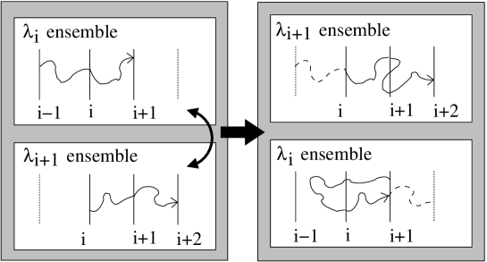
Figure 3: Path swapping move for PPTIS. The last half of the path in the $\lambda_{i}$ ensemble and the first half of the path in the $\lambda_{i+1}$ are swapped to the $\lambda_{i+1}$ and $\lambda_{i}$ ensembles, respectively.

Fig. 3 shows one path in the $\lambda_{i}$ ensemble, consisting of all possible paths crossing $\lambda_{i}$ while starting and ending at either $\lambda_{i-1}$ or $\lambda_{i+1}$, and one in the $\lambda_{i+1}$ ensemble consisting of all paths crossing $\lambda_{i+1}$ at least once, while starting and ending at either $\lambda_{i}$ or $\lambda_{i+2}$. We introduce a new MC move that attempts swapping the current path of the $\lambda_{i}$ ensemble with that of the $\lambda_{i+1}$-ensemble, as depicted in Fig. 3. The swap move will be rejected if the $\lambda_{i}$ ensemble path does not end at $\lambda_{i+1}$ or if the $\lambda_{i+1}$ ensemble path does not start at $\lambda_{i}$. Otherwise, the move is accepted and the two trajectories are swapped from one ensemble to the other. Integrating the equations of motion backward (for the $\lambda_{i}$ ensemble) and forward (for the $\lambda_{i+1}$ ensemble) will result in two entirely new paths for both ensembles. The acceptance/rejection criterion appears before any expensive computation of MD trajectories. Moreover, once accepted we obtain a new path for both ensembles for price of effectively only one path. This makes the path swapping move useful even if for systems not suffering from ergodicity problems.

Another advantage of PPS is that it allows to go beyond the pseudo-Markovian description of PPTIS. Fig. 3 shows that the paths at the right hand side, if we include the dashed trajectory part, can connect four interfaces instead of only three. This extension allows for a long range verification of the memory loss assumption. Also, the development of new, smart algorithms based on PPS might be able to correct for memory effects or to search for ideal interface positions on the fly.

While PPS is very effective when the confinement of short paths in PPTIS can cause sampling problems, even TIS and TPS algorithms might benefit from path swapping when multiple reaction channels exist.

4.2 CBMC based shooting moves

Originally developed to sample polymers at high densities, the Configurational Bias Monte Carlo (CBMC) technique grows chain molecules in a biased fashion in order to avoid unfavorable overlap of the beads [43, 44, 45, 46]. The similarity between growing polymers and generating dynamical trajectories was the inspiration for the development of TPS and has been exploited in the sampling of the stochastic path action [10, 47]. However, this CBMC-like technique was found to be less effective than the shooting algorithm [14]. Here, we propose a combination of the shooting move with CBMC for diffusive systems that suffer from low acceptance due to a non flat rough free energy barrier. When shooting from one basin of attraction in such systems, the Lyapunov instability causes the paths to diverge and return to the same basin of attraction before crossing the barrier. The use of some stochastic noise allows shooting in only one time direction and alleviates this problem slightly [48, 31], but at the price that independent pathways are generated only after a number of accepted shooting moves from the barrier region. This slow exploration of path space is even worse for processes proceeding via multiple dynamical bottlenecks, for instance reactions taking place though a short lived intermediate state

Within the shooting algorithm, CBMC can be applied both at the shooting point (the random time slice for which we change the momenta) and along the path by introducing some stochastic noise. At the shooting point $\tau^{\prime}$ we generate a set of $N_{s}$ momenta displacements $\{\delta p^{\rm(n)}\}$, and accept these displacements using step 3 in Sec. 3.3. Each phase point is then integrated forward and backward for a time $\tau_{L}$, resulting in $N_{s}$ trajectory segments ${\bf s}_{j}\equiv\{x^{(j)}_{(\tau^{\prime}-\tau_{L})\Delta t},\ldots,x^{(j)}_{(\tau^{\prime}+\tau_{L})\Delta t}\}$, for $j=1,\ldots,N_{s}$ (See Fig. 4-A). The time interval $\tau_{L}$ should be large enough to decide whether a trajectory has a chance of being successful, but much smaller than the average path length of a complete trajectory. All path segments are given a weight $w_{j}$

$$w_{j}^{\rm(n)}=\Psi\big{(}\delta p^{\rm(n)}\big{)}{\mathcal{F}}({\bf s}_{j})$$ (31)

where $\Psi$ equals 1 (else 0) for accepted momenta changes $\delta p$ at the shooting point $\tau^{\prime}$. The biasing function ${\mathcal{F}}$ should be chosen to give the highest weight $w_{j}$ to those segments that are most likely to produce a complete path of the corresponding interface ensemble. One possibility is to choose ${\mathcal{F}}=\exp(\alpha\Delta\lambda)$ with $\Delta\lambda=\lambda(x_{(\tau^{\prime}+\tau_{L})\Delta t})-\lambda(x_{(\tau^{\prime}-\tau_{L})\Delta t})$ and $\alpha$ a parameter optimized to the steepness of the barrier at $x_{\tau^{\prime}\Delta t}$. In that case, ${\mathcal{F}}$ is a function only of the backward and forward end points of the path segments ${\bf s}_{j}$.

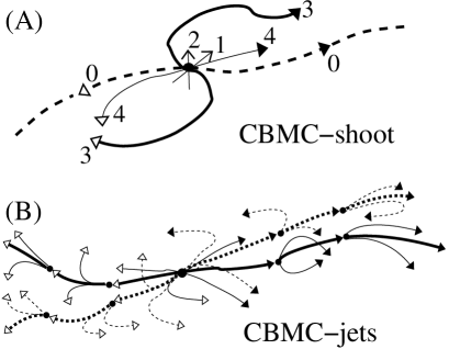
Figure 4: CBMC shooting move. (A) At the shooting point at the old trajectory (dashed line) four trial segments are released. In this example the momenta of segment 1 and 2 have been rejected and are not integrated further. Segment 0 is retracing the old path. Of the trial segments, segment 3 has come farthest in its forward (solid arrow) and backward (open arrow) time evolution and will consequently have the highest weight. (B) The use of stochasticity allows the creation of trajectory jets at several points along the path. At each junction the path will follow the most favorable direction (bold solid line). The creation of trajectory jets at the old path (bold dashed line) is required to maintain super-detailed balance.

The Rosenbluth factor for the set of trajectory segments is

$$W^{\rm(n)}\equiv\sum_{j=1}^{N_{s}}w_{j}$$ (32)

One of the segments ${\bf s}_{i}$ is selected with a probability $w_{i}/W^{\rm(n)}$. To correct for this bias and to obey detailed balance, we also have to calculate the Rosenbluth factor $W^{\rm(o)}$ for the old path. The procedure is the same as above, but now we apply $N_{s}-1$ new random momenta changes $\{\delta p^{\rm(o)}\}$ to the momenta of ${\bf s}_{i}$ at the same shooting point and again generate a set of segments of length $2\tau_{L}\Delta t$. This set is completed by adding segment ${\bf s}_{0}$ of the same length from the old path. The Rosenbluth factor for the old path equals

$$W^{\rm(o)}\equiv\sum_{j=0}^{N_{s}-1}w_{j}^{\rm(o)}.$$ (33)

where $w_{0}^{\rm(o)}$ is the weight of segment ${\bf s}_{0}$ , and $w_{j}^{\rm(o)}$ with $j=1,\ldots,N_{s}-1$ are the weights for the segments that follow from $\{\delta{p}^{\rm(o)}\}$.

By imposing super detailed balance [4] the acceptance probability of segment $i$ becomes

$$P_{\textrm{acc}}(\textrm{\bf s}_{0}\rightarrow\textrm{\bf s}_{i})=\min\left[1,\frac{w_{0}^{\rm(o)}W^{\rm(n)}\rho(x_{\tau^{\prime}\Delta t}^{\rm(n)})}{w_{i}^{\rm(n)}W^{\rm(o)}\rho(x_{\tau^{\prime}\Delta t}^{\rm(o)})}\right].$$ (34)

Here, the weight functions $w_{i}$ and the distributions $\rho$ are still present, because they do not cancel as in the standard CBMC expression. The accepted segment is integrated to the complete path just as in the normal shooting move of Sec. 3.3. Of course, this procedure is computationally more expensive than the standard shooting move. However, the biasing function ${\mathcal{F}}$ allows to choose a segment with much higher probability to become a accepted path. We expect an increase in sampling efficiency when the gain in acceptance outweighs the cost of the construction of the trajectory segment sets.

In the above algorithm we only can bias the growth of the first segment of the trajectory (the analog of the polymer in standard CBMC) because the rest of the trajectory follows deterministically once the first segment has been chosen. In the standard polymer CBMC a bias is introduced at each segment, and we can make use of the full power of CBMC if we consider stochastic trajectories. Introducing a small amount of stochasticity by for instance the Andersen thermostat [48] or by making use of the periodic boundary condition[49] will hardly change the dynamical properties of the transition process.

Stochasticity allows us to create trajectory jets at several points along the paths (See Fig. 4-B). The first segment is created as in the deterministic procedure above. However, the chosen segment is not integrated to the full path length. Instead, we start with the end point of the forward trajectory and integrate a ’jet’ of forward trajectory segments each evolving differently according to its own random noise. Each segment $j$ of this ’jet’ $k$ has a weight $w_{jk}$ similar to Eq. (31) and each jet will have a total weight $W_{k}=\sum_{j}w_{jk}$. We select a segment $i$ according to its relative weight $w_{ik}/W_{k}$, and continue with the next jet of forward segments. The same is done for the backward paths, until the path is completed. After generating the new path, we have to repeat the ’jet’ procedure for the old path as depicted in Fig. 4 in order to calculate the Rosenbluth factor of the old path. The total Rosenbluth factors are now

$$W_{RF}^{\rm(n)}=\prod_{k}W_{k}^{\rm(n)},\qquad W_{RF}^{\rm(o)}=\prod_{k}W_{k}^{\rm(o)}$$ (35)

where $k$ runs over all the jets including the one at the shooting point $x_{\tau^{\prime}\Delta t}$. The final acceptance criterion obeying super detailed balance is then

$$P_{\textrm{acc}}(o\rightarrow n)=\textrm{min}\left[1,\frac{W_{RF}^{\rm(n)}\rho(x_{\tau^{\prime}\Delta t}^{\rm(n)})\prod_{k}w_{0k}^{(o)}}{W_{RF}^{\rm(o)}\rho(x_{\tau^{\prime}\Delta t}^{\rm(o)})\prod_{k}w_{ik}^{\rm(n)}}\right]$$ (36)

where $w_{0k}^{\rm(o)}$ is the segment weight at jet $k$ on the old path and $w_{ik}^{\rm(n)}$ is the weight of the selected segment of jet $k$ on the new path. To take into account the change in path-length one should include a factor $\textrm{min}[1,N^{\rm(o)}/N^{\rm(n)}]$, but this is usually implemented by defining a maximum path length as explained at step 4 of the shooting algorithm in Sec. 3.3. The above algorithm could be useful when the standard shooting move suffers from extreme low acceptance ratios.

4.3 Time as transition parameter

In TIS the choice of the order parameter is not critical as $\lambda$ does not have to correspond to the reaction coordinate. Yet, it is possible that the order parameter $\lambda$ can bias the outcome of transition mechanism and rate constants – although much less than for the TST reactive flux method–, for instance, when the reaction mechanism leads in a direction that $\lambda$ does not allow. In principle, an order parameter-free sampling method is, therefore, highly desirable when examining unexpected contra-intuitive reaction mechanisms. One possibility for such a bias-free method is by using the time on the path outside $A$ as transition parameter (we use ’transition’ instead of ’order’ to indicate that it is not a traditional order parameter as it is not based on a phase point).

For a particular stable state $A$ definition $\lambda_{0}$, $P_{A}({\mathcal{T}}_{i+1}|{\mathcal{T}}_{i})$ is the probability that a path, starting from $\lambda_{0}$ and remaining outside $A$ over a time ${\mathcal{T}}_{i}$, remains even longer outside $A$ until at least ${\mathcal{T}}_{i+1}>{\mathcal{T}}_{i}$. To calculate the probability $P_{A}({\mathcal{T}}_{i+1}|{\mathcal{T}}_{i})$ by a bias-free TIS simulation we generate an ensemble of trajectories that have path lengths between ${\mathcal{T}}_{i}$ and ${\mathcal{T}}_{i+1}$ using the shooting algorithm of Sec. 3.3. At the shooting point, we integrate backward until reaching $\lambda_{0}$ or until the length of the trial trajectory exceeds ${\mathcal{T}}_{i+1}$ (or $N_{\rm max}^{\rm(n)}\Delta t$ as defined at step 4 of the shooting algorithm). If the backward trajectory exceeds either ${\mathcal{T}}_{i+1}$ or $N_{\rm max}^{\rm(n)}\Delta t$ the shooting move is rejected. The forward trajectory is continued until reaching $\lambda_{0}$, or until a path length of ${\mathcal{T}}_{i+1},$ or $N_{\rm max}^{\rm(n)}\Delta t$. The trial path is rejected if $N_{\rm max}^{\rm(n)}\Delta t$ is exceeded or if the trajectory ends at $\lambda_{0}$ in a time shorter than ${\mathcal{T}}_{i}$. In the subsequent ensemble, the probability $P_{A}({\mathcal{T}}_{i+2}|{\mathcal{T}}_{i+1})$ for ${\mathcal{T}}_{i+2}>{\mathcal{T}}_{i+1}$ is calculated for all paths with at least a length ${\mathcal{T}}_{i+1}$.

This method, as illustrated in Fig. 5,

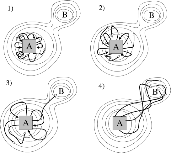
Figure 5: Time as transition parameter. The square denotes the definition of the boundary for state $A$. The thin lines are free energy contour lines. The four panels show the representation of generated trajectories in successive time-interface ensembles. At panel 1), $P_{A}({\mathcal{T}}_{i+1}|{\mathcal{T}}_{i})$ is the fraction of of trajectories that stay outside $A$ longer than ${\mathcal{T}}_{i+1}$ (open arrows). All trajectories have at least a length ${\mathcal{T}}_{i}$. The solid arrows are the paths that return to $A$ before ${\mathcal{T}}_{i+1}$. At panel 2), $P_{A}({\mathcal{T}}_{i+2}|{\mathcal{T}}_{i+1})$ is calculated for paths that remain outside $A$ longer than ${\mathcal{T}}_{i+1}$. The minimum length of the paths is further increased at panel 3). Incidentally, a path will end up in the yet unknown state $B$. At panel 4) the minimum path length constraint forces all the paths into the metastable state region $B$. From here, they will not return. Hence $P_{A}({\mathcal{T}}|0)$ will show a plateau.

will thus explore automatically the regions further and further outside $A$. At some moment it will find the closest stable state region (state $B$). Trajectories reaching this region will not go back to $A$, hence, the overall crossing probability function $P_{A}({\mathcal{T}}|0)$ will show a plateau at some time ${\mathcal{T}}$ similar to standard TIS.

Two-ended path sampling methods, such as TIS, PPTIS and TPS can only treat processes in which both stable states $A$ and $B$ are known. They cannot find the final state starting from a single stable state, a fact already discussed by Dellago and Chandler [50]. The algorithm described here, might be a solution to this problem.

5 Extracting information from path ensembles

5.1 Reaction mechanism

The ensemble of paths collected by the TIS algorithm can be used to investigate the reaction mechanism. We believe that for this purpose the TIS path ensembles might even be more useful than the TPS path ensembles. The TPS method, first samples paths that all successfully reach $B$ in the part to obtain the reactive flux function and then in the second step samples artificially short trajectories of fixed length to calculate the time correlation function C(t). Because of this constraint, the resulting ensembles do not give useful information about the reaction. The TIS $\lambda_{i}$-ensembles, on the other hand, contain the correct distribution of paths that have crossed $\lambda_{i}$ and are either going on to $\lambda_{i+1}$ or return to A. Some hidden order parameters can only be discovered by carefully comparing configurations along reactive and unreactive trajectories that are similar in terms of order parameters which at first sight were considered as being the (only) important ones. For instance, the comparison of reactive and unreactive geometries with an almost identical orientation of the reactants showed that precise tetrahedral ordering of the solvent water molecules was an important factor in the hydration reaction of ketones [30]. Although there is currently no systematic way to extract the reaction coordinates from a path ensemble, once a reaction coordinate is postulated based on physical insight it can be tested using committor distributions [13].

5.2 Activation energies

The activation energy $E_{a}$ is an important experimentally accessible quantity and is defined by the Arrhenius law

$$k=Ae^{-\beta E_{a}},$$ (37)

where A is a system dependent prefactor. In fact, $A$ and $E_{a}$ may also be temperature dependent. Such non Arrhenius behavior can be quite severe: sometimes reaction rates are even decreasing with increasing temperature, resulting in a ’negative activation energy’ (see e.g. [51]). ¿From Eq. (37) it follows that

$$E_{a}=-\frac{\partial\ln k_{AB}(\beta)}{\partial\beta}.$$ (38)

An algorithm to calculate $E_{a}$ in a TPS simulation was given in Ref. [52]. Here, we use a similar approach to calculate $E_{a}$ in a canonical TIS simulation. Substitution of Eq. (3.1) in Eq. (38) results in

$$E_{a} = -\frac{\partial}{\partial\beta}\Big{[}\ln\left\langle\phi_{1,0}\right\rangle-\ln\left\langle h_{\mathcal{A}}\right\rangle+\sum_{i=1}^{n-1}\Big{(}\ln\left\langle\Phi_{i,0}^{i+1,0}\right\rangle-\ln\left\langle\phi_{i,0}\right\rangle\Big{)}\Big{]}$$ (39)

For any function $A(x)$ we can write

$$-\frac{\partial\ln\left\langle A(x)\right\rangle}{\partial\beta}=\left\langle E(x)\right\rangle_{A}-\left\langle E(x)\right\rangle$$ (40)

with $\left\langle E(x)\right\rangle_{A}=\left\langle A(x)E(x)\right\rangle/\left\langle A(x)\right\rangle$. Using

$$\left\langle E(x)\right\rangle_{\Phi_{i,0}^{i+1,0}}=\left\langle E(x)\right\rangle_{\phi_{i+1,0}},$$ (41)

most terms in Eq. (39) cancel, only leaving

$$E_{a}=\left\langle E(x)\right\rangle_{\Phi_{n-1,0}^{n,0}}-\left\langle E(x)\right\rangle_{h_{\mathcal{A}}},$$ (42)

which is the difference between the average energy of state $A$ and the energy of the transition pathways connecting $A$ with $B$. Consequently, the calculation of the $E_{a}$ does not require all interface ensembles, but only the last ensemble $\lambda_{n-1}$. However, if all the path ensembles $i=1,\ldots,n-1$ are available an activation energy function

$$E_{a}(\lambda_{i})=\left\langle E(x)\right\rangle_{\Phi_{i-1,0}^{i,0}}-\left\langle E(x)\right\rangle_{h_{\mathcal{A}}}$$ (43)

can be calculated that should converge to a plateau analogous to the crossing probability $P(\lambda|\lambda_{1})$. A finer grid of sub-interfaces can be applied to obtain a continuous smooth function $E_{a}(\lambda)$.

Again, there is a subtle difference between the TPS and TIS algorithms. For the reaction rate determination, TPS requires a plateau in the time correlation function of Eq. (8), while TIS should give a plateau in $\lambda$ for the crossing probability $P(\lambda|\lambda_{1})$. Similarly, the TPS activation energy is expressed as a time dependent function that will converge to a plateau at times $t={\mathcal{T}}$ [52], while the TIS activation energy reaches a plateau in terms of $\lambda$.

Not all reactions show Arrhenius behavior. Therefore, it would be interesting to determine $k_{AB}(\beta)$ for a range of temperatures. One can estimate the rate for a slightly different temperature by reweighting the crossing probabilities[17, 18]. If $\left\langle A(x)\right\rangle$ is the average of an observable $A(x)$ at inverse temperature $\beta$, then $\left\langle A(x)e^{-\Delta\beta E(x)}\right\rangle/\left\langle e^{-\Delta\beta E(x)}\right\rangle$ should be the average at inverse temperature $\beta+\Delta\beta$. This reweighting technique can also be applied to the crossing probabilities (21) and the flux (28). Of course, $\Delta\beta$ should be small to obtain good enough statistics. The calculation of the temperature dependence of individual crossing probabilities has the advantage that the origin of possible non-Arrhenius behavior might be located (in terms of $\lambda$) along the reaction path.

6 Summary and Conclusions

We reviewed the basic concepts of TIS and PPTIS and explained their relation to TST based methods and TPS. We believe that path sampling methods, TPS, TIS and PPTIS, are powerful when dealing with high dimensional complex process for which is a reaction coordinate is lacking. Among these methods, TIS can be considered as an improvement upon the original TPS giving a complete non-Markovian description of the reactive event, but more efficient. PPTIS improves the efficiency even more, but relies on the assumption of memory loss between interfaces. Hence, it should only be applied for diffusive barrier crossings. In addition to this review, we have introduced several new techniques in this paper. These novel methods comprise the CBMC based shooting moves, order parameter free methods, parallel path swapping and the calculation of activation energies. The efficiency of these methods should be tested by future simulations. We plan study this in the near future.

Appendix A The flux revisited

In some cases, we can improve the efficiency of the flux calculation by separating the flux into the probability to be on the $\lambda_{1}$ surface times a factor integrating over all possible velocities when leaving the surface. The flux term can then be calculated by combining straightforward MD with, as soon as we cross the $\lambda_{1}$ surface, the sampling of sets of randomized Gaussian distributed velocities $\dot{\lambda}$, after which the MD trajectory is continued with the old original momenta. In this way, we make optimal use of the statistics of the crossing points. The velocity sampling does not require force calculations and is therefore cheap. In the following we assume that we always take $\lambda_{1}=\lambda_{0}$. Similar to Eq. (2) we can write:

$$\frac{\left\langle\phi_{1,0}\right\rangle}{\left\langle h_{\mathcal{A}}\right\rangle}=\left\langle\theta(\dot{\lambda)}\dot{\lambda}\right\rangle_{\lambda_{1}}P(\lambda_{1})_{x\in{\mathcal{A}}}$$ (44)

with

$$P(\lambda_{1})_{x\in{\mathcal{A}}}\equiv\frac{\left\langle\delta(\lambda(x)-\lambda_{1})\right\rangle}{\left\langle h_{{\mathcal{A}}}\right\rangle}$$ (45)

The two terms $\frac{\left\langle\phi_{1,0}\right\rangle}{\left\langle h_{\mathcal{A}}\right\rangle}$ and $P(\lambda_{1})_{x\in{\mathcal{A}}}$ can be obtained in the same MD simulation. As $\left\langle\delta(\lambda(x)-\lambda_{1})\right\rangle d\lambda$ is equal to the probability to find the system in the interval $[\lambda_{1}-\frac{1}{2}d\lambda:\lambda_{1}+\frac{1}{2}d\lambda]$, it can be measured by defining a width $d\lambda$ and performing a MD (or MC) simulation starting in $A$:

$$P(\lambda_{1})_{x\in{\mathcal{A}}}=\frac{1}{d\lambda}\frac{N_{\lambda_{1}}}{N_{\textrm{MD}}}$$ (46)

with $N_{\lambda_{1}}$ the number of counts in the specified interval and $N_{\textrm{MD}}$ the number of MD steps. However, this number can depend sensitively on the choice of bin width $d\lambda$. Ideally one would like $d\lambda$ to be as small as possible, at the cost of having to perform a very long simulation run for a statistically accurate number $N_{\lambda_{1}}$. A better option is to weigh the crossings with a function depending on the velocity. Assume that we cross $\lambda_{1}$ in one MD step from $x_{i\Delta t}$ to $x_{(i+1)\Delta t}$. If $d\lambda$ is small neither of these points will lie inside the interval. However, assuming a linear dynamics between these points, the system traverses from $x_{i\Delta t}$ to $x_{(i+1)\Delta t}$ in $N_{\textrm{sub}}$ equidistant sub steps. The number of phase points $N_{\lambda_{1}}$ that lie in the $d\lambda$ interval of this short linear trajectory is approximately $d\lambda N_{\textrm{sub}}/|\lambda(x_{(i+1)\Delta t})-\lambda(x_{i\Delta t})|$. The total number of MD moves $N_{\textrm{MD}}$, of course, also increases by a factor $N_{\textrm{sub}}$. So Eq.( 46) becomes

$$P(\lambda_{1})_{x\in{\mathcal{A}}}=\frac{1}{N_{\textrm{MD}}}{\sum_{i}}^{*}\frac{1}{|\lambda(x_{(i+1)\Delta t})-\lambda(x_{i\Delta t})|}$$ (47)

where the $*$ indicates that the summation has to be performed only for points $i$ along the trajectory for which $x_{i\Delta t}\rightarrow x_{(i+1)\Delta t}$ showed a crossing (positive or negative) with interface $\lambda_{1}$. Further optimization can be achieved by writing $|\lambda(x_{(i+1)\Delta t})-\lambda(x_{i\Delta t})|=|\dot{\lambda}_{x_{i\Delta t}}|\Delta t+{\mathcal{O}}(\Delta t^{2})=|\dot{\lambda}_{x_{(i+1)\Delta t}}|\Delta t+{\mathcal{O}}(\Delta t^{2})$, but the velocity $\dot{\lambda}$ at the interface would give the most exact result. If we also assume a linear change in time for the velocities between $i$ and $i+1$, our best estimate for $P(\lambda_{1})_{x\in{\mathcal{A}}}$ is:

$$P(\lambda_{1})_{x\in{\mathcal{A}}} = \frac{1}{N_{\textrm{MD}}\Delta t}{\sum_{i}}^{*}\frac{1}{|\dot{\lambda}(x_{i\Delta t};\lambda_{1})|}$$ (48)

where we have introduced the notation $g(x_{i\Delta t};\lambda_{j})$ to denote the function $g(x)$ at the crossing point of interface $\lambda_{j}$ obtained by a linear interpolation of the function between two successive trajectory points $x_{i\Delta t}\rightarrow x_{(i+1)\Delta t}$:

$$g(x_{i\Delta t};\lambda_{j}) \equiv \frac{1}{\lambda(x_{(i+1)\Delta t})-\lambda(x_{i\Delta t})}\big{\{}[\lambda(x_{(i+1)\Delta t})-\lambda_{j}]g(x_{i\Delta t})+[\lambda_{j}-\lambda(x_{i\Delta t})]g(x_{(i+1)\Delta t})\big{\}}$$

The factor $\left\langle\theta(\dot{\lambda})\dot{\lambda}\right\rangle_{\lambda_{1}}$ in Eq. (44) can be calculated in the same MD simulation with an additional sampling procedure. In some simple cases, there is even an analytically expression. For instance, in case the $x$-coordinate of particle $j$ is the order parameter, $\lambda(x)=r_{jx}$ in a constant temperature (NVT) simulation, we would obtain $\left\langle\theta(\dot{\lambda})\dot{\lambda}\right\rangle_{\lambda_{1}}=\frac{1}{\sqrt{2\pi\beta m_{j}}}$ with $m_{j}$ the mass of this particle. However, for more complex $\lambda(x)$, such as the distance between two particles $i$ and $j$, $\lambda(x)=|r_{i}-r_{j}|$, no simple analytic expression exists. The calculation of $\left\langle\theta(\dot{\lambda})\dot{\lambda}\right\rangle_{\lambda_{1}}$ can then be calculated by sampling a random set of $N_{\textrm{MC}}$ velocities $\dot{\lambda}$ as soon as a crossing is detected:

$$\left\langle\theta(\dot{\lambda})\dot{\lambda}\right\rangle_{\lambda_{1}}=\frac{{\sum_{i}}^{*}\Big{[}\frac{1}{|\dot{\lambda}(x_{i\Delta t};\lambda_{1})|}\sum_{j}^{N_{\textrm{MC}}}\theta(\dot{\tilde{\lambda}})\dot{\tilde{\lambda}}\Big{]}}{N_{\textrm{MC}}{\sum_{i}}^{*}\Big{[}\frac{1}{|\dot{\lambda}(x_{i\Delta t};\lambda_{1})|}\Big{]}}$$ (50)

where $i$ runs over all MD crossings with interface $\lambda_{1}$, $\dot{\lambda}(x_{i\Delta t};\lambda_{1})$ is the MD crossing velocity through $\lambda_{1}$, $j$ runs over the $N_{\textrm{MC}}$ ’artificial’ velocities $\dot{\tilde{\lambda}}$ that are taken from a proper distribution $P(\dot{\tilde{\lambda}}|x_{i\Delta t})$. For NVT simulations without additional constraints this distribution $P(\dot{\tilde{\lambda}}|x_{i\Delta t})$ does not depend on the phase point $x_{i\Delta t}$ and we can simply sample $\dot{\tilde{\lambda}}(\{p\})$ where the momenta $\{p\}$ defining $\dot{\lambda}$ are taken from a Gaussian distribution For NVE simulations, the distribution $P(\dot{\tilde{\lambda}}|x_{i\Delta t})$ does depend $x_{i\Delta t}$ and we have to change all momenta and distribute them on the hypersphere defined by the kinetic energy $K=E-V(x_{i\Delta t};\lambda_{1})$ with $E$ the total energy and $V(x_{i\Delta t};\lambda_{1})$ the total potential energy at the crossing point. The proper sampling of momenta distributions in the presence of linear constraints, such as linear and angular momentum is explained in Ref. [37]. Clearly, if $P(\dot{\tilde{\lambda}}|x_{i\Delta t})=\delta\big{(}\dot{\tilde{\lambda}}-\dot{\lambda}(x_{i\Delta t};\lambda_{1})\big{)}$, Eq. (50) would be equal to $N_{c}^{+}/{\sum_{i}}^{*}|\dot{\lambda}(x_{i\Delta t};\lambda_{1})|^{-1}$ leaving Eq. (44) identical to Eq. (28) from which we started.

Appendix B TIS shooting acceptance criterion for stochastic dynamics

Although we assume throughout the paper that the equations of motion were deterministic, it is sometimes useful to implement some stochasticity into the dynamics, or consider completely stochastic equation of motion such as Brownian Dynamics [14, 48, 31]. Quantities like $\bar{h}_{\mathcal{A}}(x_{0})$ are, then, no longer just 1 or 0 but turn into probabilities with a fractional value. Moreover, for stochastic dynamics it is not trivial whether we are allowed to use the path that generated $x_{0}^{\rm(o)}$ as our instrument to search for the new phase point $x_{0}^{\rm(n)}$. In this appendix we derive the acceptance probability for the shooting algorithm for arbitrary dynamics along the same lines as in Ref. [14]. At start, we try to be as general as possible making the least possible assumptions on the type of dynamics or on whether the system is in equilibrium or not. For this purpose, it is most convenient to use the path space description, instead of phase space. The weight or probability density ${\mathcal{P}}[{\bf x}]$ for a single path ${\bf x}\equiv\{x_{-\tau^{b}\Delta t},\ldots;x_{0}~{};\ldots,x_{+\tau^{f}\Delta t}\}$ is than not only determined by the distribution $\rho(x_{0})$ of $x_{0}$, but also by the probabilities of arriving along this precise route from $x_{-\tau^{b}\Delta t}$ in the past and continuing upto $x_{+\tau^{f}\Delta t}$ in the future.

$${\mathcal{P}}[{\bf x}]=\rho(x_{0})\prod_{i=-1}^{-\tau^{b}}p(x_{(i+1)\Delta t}\leftarrow x_{i\Delta t})\prod_{i=1}^{\tau^{f}}p(x_{(i-1)\Delta t}\rightarrow x_{i\Delta t})$$ (51)

where $p(x\rightarrow y)$ is the forward transition probability (more accurate: probability density) to go from $x$ to $y$ and $p(y\leftarrow x)$ is the probability that, if the system is at $y$, it came from $x$ in the past. Here, $\rho(x_{0})$ is not necessarily the Boltzmann distribution or even a distribution in equilibrium. It is applicable to all systems that (at least to some approximation) are described by a steady state. We can express $p(y\leftarrow x)$ in terms of forward transition probabilities as

$$p(y\leftarrow x)=\frac{\rho(x)p(x\rightarrow y)}{\int\mathrm{d}x^{\prime}\rho(x^{\prime})p(x^{\prime}\rightarrow y)}=\frac{\rho(x)p(x\rightarrow y)}{\rho(y)}.$$ (52)

where $\int\mathrm{d}x^{\prime}\rho(x^{\prime})p(x^{\prime}\rightarrow y)=\rho(y)$ results from the steady state behavior. Using this relation, one can show that Eq. (51) is exactly equal to the probability of the first point $\rho(x_{-\tau^{b}\Delta t})$ times the forward evolution probabilities

$${\mathcal{P}}[{\bf x}]=\rho(x_{-\tau^{b}\Delta t})\prod_{i=-\tau^{b}}^{\tau^{f}-1}p(x_{i\Delta t}\rightarrow x_{(i+1)\Delta t})$$ (53)

which is identical to the weight for a path in the TPS-ensemble [14] with $x_{-\tau^{b}\Delta t}$ instead of $x_{0}$. Note that so far, we have assumed nothing about the nature of dynamics (irreversible or reversible, stochastic or deterministic). When restricted to the TIS ensemble for interface $i$, the probability density of a path can be written as

$${\mathcal{P}}_{\lambda_{i}}[{\bf x}]\equiv\hat{h}_{i}({\bf x}){\mathcal{P}}[{\bf x}]/Z(\lambda_{i})$$ (54)

where $\hat{h}_{i}$ is unity if the path goes from $\lambda_{0}$, crosses $\lambda_{i}$ and ends either at $\lambda_{i+i}$ or goes back to $\lambda_{0}$. Otherwise it is zero. The normalizing factor $Z(\lambda_{i})$ equals

$$Z(\lambda_{i})\equiv\int\!\mathcal{D}{\bf x}\,\hat{h}_{i}({\bf x}){\mathcal{P}}[{\bf x}]$$ (55)

where the integral is taken over all possible paths ${\bf x}$ of all lengths, starting in all possible initial conditions $x_{-\tau_{b}}$. Note that, contrary to TPS, Eq. (53) and Eq. (54) are not directly related to the relative probabilities of all paths in the TIS ensemble. This is a result of the path ensemble containing paths of different lengths. Eq. (53) turns into a true probability only when multiplied with the infinitesimal volume element in path space $\mathcal{D}{\bf x}\equiv\prod_{i=-\tau^{b}}^{\tau^{f}}\mathrm{d}x_{i\Delta t}\sim\mathrm{d}x^{N}$. Hence, a long path has an infinitely smaller probability than a shorter one for stochastic dynamics. Therefore, the concept of path space may sound peculiar for TIS. Still, it is instrumental to derive proper acceptance rules for TIS obeying detailed balance.

When performing the random walk in the TIS path space using the shooting algorithm, the detailed balance condition is

$$\frac{P_{\textrm{gen}}[{\bf x}^{\rm(o)}\rightarrow{\bf x}^{\rm(n)}]}{P_{\textrm{gen}}[{\bf x}^{\rm(n)}\rightarrow{\bf x}^{\rm(o)}]}\frac{P_{\textrm{acc}}[{\bf x}^{\rm(o)}\rightarrow{\bf x}^{\rm(n)}]}{P_{\textrm{acc}}[{\bf x}^{\rm(n)}\rightarrow{\bf x}^{\rm(o)}]}=\frac{{\mathcal{P}}_{\lambda_{i}}[{\bf x}^{\rm(n)}]}{{\mathcal{P}}_{\lambda_{i}}[{\bf x}^{\rm(o)}]}$$ (56)

where o and n, denote the old and new path respectively. The usual Metropolis acceptance rule is then

$$P_{\rm acc}[{\bf x}^{\rm(o)}\rightarrow{\bf x}^{\rm(n)}]=\hat{h}_{i}({\bf x}^{\rm(n)})\min\left[1,\frac{{\mathcal{P}}[{\bf x}^{\rm(n)}]}{{\mathcal{P}}[{\bf x}^{\rm(o)}]}\frac{P_{\rm gen}[{\bf x}^{\rm(n)}\rightarrow{\bf x}^{\rm(o)}]}{P_{\rm gen}[{\bf x}^{\rm(o)}\rightarrow{\bf x}^{\rm(n)}]}\right],$$ (57)

Note that this rule only applies at the trajectory space level, it has nothing to do with whether the underlying dynamics is stochastic or deterministic, or even reversible or irreversible.

The generation probability to create a new path from an old path using the shooting move is given by

$${P_{\rm gen}[{\bf x}^{\rm(o)}\rightarrow{\bf x}^{\rm(n)}])]} = \frac{P(\delta p)}{N^{\rm(o)}}P_{\rm gen}^{\rm f}[{\bf x}^{\rm(o)}\rightarrow{\bf x}^{\rm(n)}]P_{\rm gen}^{\rm b}[{\bf x}^{\rm(o)}\rightarrow{\bf x}^{\rm(n)}]$$ (58)

where $1/N^{\rm(o)}$ is the chance to choose the shooting point $\tau^{\prime}$ with $-\tau^{b{\rm(o)}}\leq\tau^{\prime}\leq\tau^{f{\rm(o)}}$) at the old path, $P(\delta p)$ the chance to select the randomized momenta displacements. As $\delta p$ is normally taken from a symmetric distribution, hence $P(\delta p)=P(-\delta p)$, this term will cancel in Eq. (57). The last two factors in Eq. (58) are the probabilities to generate trajectories from the shooting point point $\tau^{\prime}$ with the new momenta. These generation probabilities are given by the underlying dynamics used to generate the trajectories. If one starts from a shooting point at $\tau^{\prime}$ on the old existing path (with $-\tau_{b}^{\rm(o)}<\tau^{\prime}<\tau_{f}^{\rm(o)}$) the generation probability for the forward segment is

$$P_{\rm gen}^{\rm f}[{\bf x}^{\rm(o)}\rightarrow{\bf x}^{\rm(n)}]=\prod_{i=\tau^{\prime}}^{\tau_{f}^{\rm(n)}-1}p\left(x_{i\Delta t}^{\rm(n)}\rightarrow x_{(i+1)\Delta t}^{\rm(n)}\right).$$ (59)

This generation probability is exactly identical to the weight of the forward segment. The integration of the backward segment is not always trivial especially when dealing with irreversible processes. However, in general, when reversible dynamics is applied, the backward segment is obtained by reversing the momenta, integrating forward in time and reversing the momenta again [14]. Accordingly, the backward segment’s generation probability equals

$$P_{\rm gen}^{\rm b}[{\bf x}^{\rm(o)}\rightarrow{\bf x}^{\rm(n)}]=\prod_{i=-\tau_{b}^{\rm(n)}}^{\tau^{\prime}-1}p\left(\bar{x}_{(i+1)\Delta t}^{\rm(n)}\rightarrow\bar{x}_{i\Delta t}^{\rm(n)}\right).$$ (60)

where $\bar{x}\equiv\{r,-p\}$ for a phase point $x\equiv\{r,p\}$. Using these generation probabilities and the path weight Eq. (53) the factor within the min function of Eq (57) can be written as

$$\frac{{\mathcal{P}}[{\bf x}^{\rm(n)}]P_{\rm gen}[{\bf x}^{\rm(n)}\rightarrow{\bf x}^{\rm(o)}]}{{\mathcal{P}}[{\bf x}^{\rm(o)}]P_{\rm gen}[{\bf x}^{\rm(o)}\rightarrow{\bf x}^{\rm(n)}]}=\frac{\rho[x_{-\tau_{b}^{\rm\rm(n)}}]N^{\rm(o)}}{\rho[x_{-\tau_{b}^{\rm(o)}}]N^{\rm(n)}}\times$$

$$\prod_{i=-\tau_{b}^{\rm(n)}}^{\tau^{\prime}-1}\frac{p[x_{i\Delta t}^{\rm(n)}\rightarrow x_{(i+1)\Delta t}^{\rm(n)}]}{p[\bar{x}_{(i+1)\Delta t}^{\rm(n)}\rightarrow\bar{x}_{i\Delta t}^{\rm(n)}]}\prod_{i=-\tau_{b}^{\rm(o)}}^{\tau^{\prime}-1}\frac{p[\bar{x}_{(i+1)\Delta t}^{\rm(o)}\rightarrow\bar{x}_{i\Delta t}^{\rm(o)}]}{p[x_{i\Delta t}^{\rm(o)}\rightarrow x_{(i+1)\Delta t}^{\rm(o)}]}.$$

where the generation probability and the weight of the forward parts of the trajectories have canceled each other. Eq. (53) simplifies tremendously for dynamics that obey the microscopic reversibility condition [14]

$$\frac{p(x\rightarrow y)}{p(\bar{y}\rightarrow\bar{x})}=\frac{\rho(y)}{\rho(x)}.$$ (62)

This condition can be seen as a special case of Eq. (52) for time-reversible dynamics with $p(y\leftarrow x)=p(\bar{y}\rightarrow\bar{x})$, but is very general and valid for a broad class of dynamics applying to both equilibrium and non-equilibrium systems. As result, if the microscopic reversibility condition (62) is satisfied and thus $p(\bar{y}\rightarrow\bar{x})=p(y\leftarrow x)$, almost all terms in Eq. (B) cancel, except for the steady state distributions $\rho(x_{\tau^{\prime}})$ of the shooting points.

$$P_{\rm acc}[{\bf x}^{\rm(o)}\rightarrow{\bf x}^{\rm(n)}]=\hat{h}_{i}({\bf x}^{\rm(n)})\min\left[1,\frac{\rho(x_{\tau^{\prime}}^{\rm(n)})}{\rho(x_{\tau^{\prime}}^{\rm(o)})}\frac{N^{\rm(o)}}{N^{\rm(n)}}\right].$$ (63)

which is exactly the same as for deterministic dynamics.

This is an important result as it allows to perform the acceptance/rejection rule (step 3 of Sec. 3.3) for the new momenta at the shooting point even if the energy along the path changes giving a different weight to $\rho(x_{\tau^{\prime}\Delta t})$ as to $\rho(x_{0})$. The ratio $N^{\rm(o)}/N^{\rm(n)}$ in Eq. (63) can, of course, not be known in advance at the shooting point. However, this is effectively circumvented by defining $N_{\rm max}$ at step 4 of the shooting algorithm in Sec. 3.3 leaving only the $\rho(x_{\tau^{\prime}}^{\rm(n)})/\rho(x_{\tau^{\prime}}^{\rm(o)})$ term for the acceptance rule (step 3).

References

- [1] A. R. Leach, Molecular Modeling: Principles and Applications, Pearson Education, Harlow, England, 2001.
- [2] R. Car, M. Parrinello, Unified approach for molecular dynamics and density-functional theory, Phys. Rev. Lett. 55 (1985) 2471–2474.
- [3] M. Allen, D. Tildesley, Computer Simulation of Liquids, Clarendon Press, Oxford, 1987.
- [4] D. Frenkel, B. Smit, Understanding Molecular Simulation, 2nd ed., Academic Press, San Diego, CA, 2002.
- [5] D. Chandler, Introduction to Modern Statistical Mechanics, Oxford University, New York, 1987.
- [6] J. C. Keck, Discuss. Faraday Soc. 33 (1962) 173.
- [7] J. B. Anderson, Statistical-theories of chemical reactions - distributions in transition region, J. Chem. Phys. 58 (1973) 4684–4692.
- [8] C. H. Bennett, Molecular dynamics and transition state theory: the simulation of infrequent events, in: R. E. Christofferson (Ed.), Algorithms for Chemical Computations, ACS Symposium Series No. 46, American Chemical Society, Washington, D. C., 1977, pp. 63–97.
- [9] D. Chandler, Statistical-mechanics of isomerization dynamics in liquids and transition-state approximation, J. Chem. Phys. 68 (1978) 2959–2970.
- [10] C. Dellago, P. G. Bolhuis, F. S. Csajka, D. Chandler, Transition path sampling and the calculation of rate constants, J. Chem. Phys. 108 (1998) 1964–1977.
- [11] P. G. Bolhuis, C. Dellago, D. Chandler, Sampling ensembles of deterministic transition pathways, Faraday Discuss. 110 (1998) 421–436.
- [12] C. Dellago, P. G. Bolhuis, D. Chandler, On the calculation of reaction rate constants in the transition path ensemble, J. Chem. Phys. 110 (1999) 6617–6625.
- [13] P. G. Bolhuis, D. Chandler, C. Dellago, P. Geissler, Transition path sampling: Throwing ropes over rough mountain passes, in the dark, Annu. Rev. Phys. Chem. 53 (2002) 291–318.
- [14] C. Dellago, P. G. Bolhuis, P. L. Geissler, Transition path sampling, Adv. Chem. Phys. 123 (2002) 1–78.
- [15] T. S. van Erp, D. Moroni, P. G. Bolhuis, A novel path sampling method for the sampling of rate constants, J. Chem. Phys. 118 (2003) 7762–7774.
- [16] D. Moroni, P. G. Bolhuis, T. S. van Erp, Rate constants for diffusive processes by partial path sampling, J. Chem. Phys. 120 (2004) 4055–4065.
- [17] G. M. Torrie, J. P. Valleau, Monte-carlo study of a phase-separating liquid-mixture by umbrella sampling, Chem. Phys. Lett. 28 (1974) 578–581.
- [18] E. A. Carter, G. Ciccotti, J. T. Hynes, R. Kapral, Constrained reaction coordinate dynamics for the simulation of rare events, Chem. Phys. Lett. 156 (1989) 472–477.
- [19] G. Ciccotti, Molecular Dynamics simulations of nonequilibrium phenomena and rare dynamical events, in: M. Meyer, V. Pontikis (Eds.), Computer Simulations in Materials Science, Kluwer, Dordrecht, 1991, pp. 365–396.
- [20] T. Yamamoto, Quantum statistical mechanical theory of the rate of exchange chemical reactions in the gas phase, J. Chem. Phys. 33 (1960) 281–289.
- [21] J. P. Bergsma, J. R. Reimers, K. R. Wilson, J. T. Hynes, Molecular dynamics of the a+bc reaction in rare gas solution, J. Chem. Phys. 85 (1986) 5625–5643.
- [22] B. J. Berne, Molecular dynamics and monte carlo simulations of rare events, in: J. U. Brackbill, B. I. Cohen (Eds.), Multiple Time Scales, Academic Press, Orlando, 1985, pp. 419–436.
- [23] G. W. N. White, S. Goldman, C. G. Gray, Test of rate theory transmission coefficients algorithms. an application to ion channels, Mol. Phys. 98 (2000) 1871–1885.
- [24] G. Hummer, From transition paths to transition states and rate coefficients, J. Chem. Phys. 120 (2004) 516–523.
- [25] M. J. Ruiz-Montero, D. Frenkel, J. J. Brey, Efficient schemes to compute diffusive barrier crossing rates, Mol. Phys. 90 (1997) 925–941.
- [26] J. B. Anderson, Predicting rare events in molecular dynamics, Adv. Chem. Phys. 91 (1995) 381–431.
- [27] T. S. van Erp, Solvent effects on chemistry with alcohols, Ph.D. thesis, Universiteit van Amsterdam (2003).
- [28] M. Sprik, Coordination numbers as reaction coordinates in constrained molecular dynamics, Farady Discuss. 110 (1998) 437–445.
- [29] M. Sprik, Computation of the pk of liquid water using coordination constraints, Chem. Phys. 258 (2000) 139–150.
- [30] T. S. van Erp, E. J. Meijer, Proton assisted ethylene hydration in aqueous solution, Angew. Chemie 43 (2004) 1660–1662.
- [31] P. G. Bolhuis, Transition-path sampling of beta-hairpin folding, Proc. Natl. Acad. Sci. USA 100 (2003) 12129–12134.
- [32] S. Nosé, A unified formulation of the constant temperature molecular dynamics method, J. Chem. Phys. 81 (1984) 511–519.
- [33] S. Nosé, A molecular dynamics method for simulation in the canonical ensemble, Mol. Phys. 52 (1984) 255–268.
- [34] W. G. Hoover, Canonical dynamics - equilibrium phase-space distributions, Phys. Rev. A 31 (1985) 1695–1697.
- [35] G. J. Martyna, M. E. Tuckerman, D. J. Tobias, M. L. Klein, Explicit reversible integrators for extended systems dynamics, Mol. Phys. 87 (1996) 1117–1157.
- [36] H. C. Andersen, Molecular dynamics at constant pressure and/or temperature, J. Chem. Phys. 72 (1980) 2384–2393.
- [37] P. L. Geissler, C. Dellago, D. Chandler, Chemical dynamics of protonated water trimer analyzed by transition path sampling, Phys. Chem. Chem. Phys. 1 (1999) 1317–1322.
- [38] S. Duane, A. D. Kennedy, B. J. Pendleton, D. Roweth, Hybrid monte carlo, Phys. Lett. B 195 (1987) 216–222.
- [39] W. C. Swope, H. C. Andersen, P. H. Berens, K. R. Wilson, A computer simulation method for the calculation of equilibrium constants for the formation of physical clusters of molecules, J. Chem. Phys. 76 (1982) 637–649.
- [40] B. A. Berg, T. Neuhaus, Multicanonical ensemble - a new approach to simulate 1st-order phase-transitions, Phys. Rev. Lett. 68 (1992) 9–12.
- [41] B. Ensing, E. J. Meijer, P. E. Blöchl, E. J. Baerends, Solvation effects on the s(n)2 reaction between ch3cl and cl- in water, J. Phys. Chem. A 105 (2001) 3300–3310.
- [42] T. J. H. Vlugt, B. Smit, On the efficient sampling of pathways in the transition path ensemble, Phys. Chem. Comm. 2 (2001) 1.
- [43] M. N. Rosenbluth, A. W. Rosenbluth, Monte-carlo calculation of the average extension of molecular chains, J. Chem. Phys. 23 (1955) 356–359.
- [44] J. I. Siepmann, D. Frenkel, Configurational bias monte-carlo - a new sampling scheme for flexible chains, Mol. Phys. 75 (1992) 59–70.
- [45] J. J. de Pablo, M. Laso, U. W. Suter, Simulation of polyethylene above and below the melting-point, J. Chem. Phys. 96 (1992) 2395–2403.
- [46] D. Frenkel, G. C. A. M. Mooij, B. Smit, Novel scheme to study structural and thermal-properties of continuously deformable molecules, J. Phys.: Condens. Matter 4 (1992) 3053–3076.
- [47] F. S. Csajka, D. Chandler, Transition pathways in a many-body system: Application to hydrogen-bond breaking in water, J. Chem. Phys. 109 (1998) 1125–1133.
- [48] P. G. Bolhuis, Transition path sampling on diffusive barriers, J. of Phys. Cond. Matter 15 (2003) S113–S120.
- [49] G. Ciccotti, A. Tenenbaum, Canonical ensemble and nonequilibrium states by molecular dynamics, J. Stat. Phys. 23 (1980) 767–772.
- [50] C. Dellago, D. Chandler, Bridging the time scale gap with transition path sampling, in: P. Nielaba, M. Mareschal, G. Ciccotti (Eds.), Molecular Simulation for the Next Decade, Vol. 605 of Lecture Notes in Physics (LNP), Springe, Berlin, 2002, pp. 321–333.
- [51] T. Shimomur, K. J. Tolle, J. Smid, M. Szwarc, Energy and entropy of activation of propagation by free polystyryl anions and their ion pairs . phenomenon of negative activation energy, J. Am. Chem. Soc. 89 (1967) 796.
- [52] C. Dellago, P. G. Bolhuis, Activation energies from transition path sampling simulations, Mol. Sim.