[

Quantitative comparison between theoretical predictions and experimental results for the BCS-BEC crossover

Abstract

Theoretical predictions for the BCS-BEC crossover of trapped Fermi atoms are compared with recent experimental results for the density profiles of ⁶Li. The calculations rest on a single theoretical approach that includes pairing fluctuations beyond mean field. Excellent agreement with experimental results is obtained. Theoretical predictions for the zero-temperature chemical potential and gap at the unitarity limit are also found to compare extremely well with Quantum Monte Carlo simulations and with recent experimental results.

PACS number(s): 03.75.Hh,03.75.Ss

]

The original theoretical ideas behind the crossover, from the Bardeen-Cooper-Schrieffer (BCS) superconductivity with largely overlapping Cooper pairs to the Bose-Einstein condensation (BEC) of dilute bosons, date back to the pioneering work by Eagles for low-carrier doped superconductors [1]. Later seminal papers by Leggett and by Nozières and Schmitt-Rink have provided a general framework for the BCS-BEC crossover, both at zero temperature in the superfluid phase [2] and at finite temperature in the normal phase [3]. The experimental motivations to these studies came from the condensation of excitons in solids [4], pairing in nuclei [5], and pseudogap in high-temperature superconductors [6]. No direct quantitative comparison between theory and experiments has, however, been possible so far, owing essentially to the large number of degrees of freedoms present in these systems.

Recent experimental advances on the condensation of ultracold trapped Fermi atoms [7] make it now possible to compare theoretical predictions for the BCS-BEC crossover with experimental results. In these systems, the use of a tunable Fano-Feshbach (FF) resonance [8] provides the fermionic attraction that triggers pairing, thus enabling one to pass with continuity from weak (BCS) to strong (BEC) coupling across the crossover region. In addition, for broad enough resonances, the scattering length $a_{F}$ appears to be the only relevant quantity entering the many-body Hamiltonian of the interacting Fermi atoms [9]. Experiments on ultracold Fermi atoms thus constitute an ideal testing ground for theories which describe the progressive quenching of the fermionic degrees of freedom into composite bosons.

Comparison of theory with experiments is more interesting for the BCS-BEC crossover with Fermi atoms than for the BEC with Bose atoms. This is because the diluteness condition for Bose gases makes it appropriate to describe the bosonic condensate by the Gross-Pitaevskii equation [10] and the excitations above it by the Bogoliubov approximation [11]. For the BCS-BEC crossover, on the other hand, many-body approximations can be controlled only on the two (BCS and BEC) sides of the crossover, where the diluteness condition holds for the gas of fermions and composite bosons, respectively. A small parameter to control the many-body approximations is instead lacking in the intermediate (crossover) region where the scattering length $a_{F}$ diverges.

Any sensible theoretical approach to crossover phenomena sets up a single theory that recovers controlled approximations on both sides of the crossover and provides a continuous evolution between them. It is then of particular relevance that for the BCS-BEC crossover the results for the intermediate-coupling regime can be compared with accurate results from Quantum Monte Carlo (QMC) simulations [12] performed at the unitarity limit where $a_{F}$ diverges. This provides a further stringent test on the validity of a BCS-BEC crossover theory.

Characteristic of any BCS-BEC crossover theory is to provide two coupled equations for the order parameter $\Delta$ and the chemical potential $\mu$ (the latter being strongly renormalized from one limit to the other). In the present theory for the trapped gas, these equations are obtained by considering a local-density approximation to the theory of Ref. [13]. The overall chemical potential is replaced whenever it occurs by the local quantity $\mu({\mathbf{r}})=\mu-V({\mathbf{r}})$ that includes the trapping potential $V({\mathbf{r}})$ at position ${\mathbf{r}}$, as discussed in Ref.[14]. In Ref. [13], the theory developed by Popov for a weakly-interacting (dilute) superfluid Fermi gas [15] was extended as to include the effects of the collective Bogoliubov-Anderson mode [16] in the diagonal fermionic self-energy. This was obtained by considering the self-energy (with Nambu notation)

$$\Sigma_{11}(k) = -\int\frac{d{\bf q}}{(2\pi)^{3}}\;T\sum_{\nu}\Gamma_{11}(q){\mathcal{G}}_{11}(q-k)$$ (1)

$$\Sigma_{12}(k) = -\Delta,$$ (2)

where $\Gamma_{11}(q)=\chi_{11}(-q)/[\chi_{11}(q)\chi_{11}(-q)-\chi_{12}(q)^{2}]$ is the normal pair propagator with

$$-\,\chi_{11}(q) = \frac{m}{4\pi a_{F}}+\int\frac{d{\mathbf{k}}}{(2\pi)^{3}}\,\left[\;T\sum_{n}\,{\mathcal{G}}_{11}(k+q)\,{\mathcal{G}}_{11}(-k)\right.$$ (4)

$$\phantom{\frac{m}{4\pi a_{F}}}-\left.\frac{m}{{\bf k}^{2}}\right]$$

$$\chi_{12}(q) = \int\!\frac{d{\mathbf{k}}}{(2\pi)^{3}}\,\;T\sum_{n}\,{\mathcal{G}}_{12}(k+q)\,{\mathcal{G}}_{21}(-k).$$ (5)

In these expressions, $q=({\mathbf{q}},\Omega_{\nu})$ and $k=({\mathbf{k}},\omega_{n})$ (${\mathbf{q}}$ and ${\mathbf{k}}$ are wave vectors, $\Omega_{\nu}$ and $\omega_{n}$ bosonic and fermionic Matsubara frequencies, respectively), $m$ is the fermion mass, $T$ the temperature, and ${\mathcal{G}}_{ij}$ $(i,j=1,2)$ are BCS Green’s functions. (We set $\hbar$=$k_{B}$=1 throughout.)

In the BCS limit, the quantity $k_{F}a_{F}$ ($a_{F}<0$) identifies the small parameter needed to control the approximations. Here, the Fermi wave vector $k_{F}$ is obtained by setting $k_{F}^{2}/(2m)$ equal to the Fermi energy $E_{F}$ of the non-interacting Fermi gas. The scattering length $a_{F}$ is varied in experiments with trapped Fermi atoms from negative to positive values across the FF resonance where $a_{F}$ diverges. It was predicted [14, 17] that the crossover from fermionic to bosonic behavior in a trap occurs, in practice, within the narrow range $-1\lesssim(k_{F}a_{F})^{-1}\lesssim 1$. By our generalization of the Popov fermionic approximation, in the strong-coupling limit of the fermionic attraction the same fermionic theory is able to describe a dilute system of composite bosons within the Bogoliubov approximation [11]. In this limit, the small parameter $k_{F}a_{F}$ ($a_{F}>0$) corresponds to the “gas parameter” of the dilute Bose gas.

Experiments with trapped Fermi atoms are usually made using anisotropic harmonic trapping potentials, having different frequencies $\omega_{x}$, $\omega_{y}$, and $\omega_{z}$ for the three axis. In this case, the Fermi energy $E_{F}$ equals $(3N\omega_{x}\omega_{y}\omega_{z})^{1/3}$ where $N$ is the total number of Fermi atoms in the trap. Within a local-density approximation, the anisotropic problem can be readily mapped onto a corresponding isotropic problem with the same value of the Fermi energy. Detailed experimental axial density profiles for ⁶Li Fermi atoms were reported in Ref. [18] across the intermediate (crossover) region of interest. In Ref. [18], $\omega_{x}=\omega_{y}=\omega_{r}$ and $\omega_{z}=\lambda\omega_{r}$ with $\lambda\ll 1$. The experimental values of $\omega_{r}$, $\omega_{z}$, $a_{F}$, and $N$ determine the value of $(k_{F}a_{F})^{-1}$, to be used for comparison with the theoretical calculations. In addition, for the experiments reported in Ref. [18] the temperature is estimated to be much smaller than $E_{F}$. Correspondingly, the theoretical calculations can be performed at $T=0$.

Figure 1 shows the comparison between our theoretical predictions for the axial density profiles in the crossover region and the data reported in Fig. 4 of Ref. [18], for three different values of the magnetic field $B$ tuning the FF resonance. The intermediate value $B=850G$ (about) corresponds to the position of the resonance at which $a_{F}$ diverges. For the two other values $B=882G$ and $B=809G$, the values of the scattering length are estimated to be $a_{F}=-1.8\times 10^{4}a_{0}$ and $a_{F}=8.5\times 10^{3}a_{0}$, respectively, where $a_{0}$ is the Bohr radius. These values are extracted from the data reported in Fig. 3(a) of Ref. [18]. The value of $k_{F}$ is obtained with $\omega_{r}/(2\pi)=640Hz$ and $\omega_{z}/(2\pi)=\sqrt{0.6\times B[G]+32}Hz$, and depends weakly on the estimated value of $N$ which is affected by the largest experimental uncertainty (of the order of $50\%$).

         

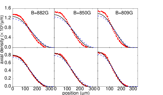
FIG. 1.: Comparison between experimental and theoretical axial density profiles. Experimental data from Ref. 18 (dots) are shown for three diffeent values of the magnetic field $B$ tuning the FF resonance. Theoretical results at $T=0$ obtained by our theory (full lines) and by BCS mean field (dashed lines) are shown for the corresponding couplings $(k_{F}a_{F})^{-1}$ given in the text. The upper (lower) panel refers to the estimated number of atoms $N=4\times 10^{5}$ ($N=2.3\times 10^{5}$).

This uncertainty affects only the absolute scale of the experimental density profiles but not their shape. The upper panel of Fig. 1 corresponds to the estimated value $N=4\times 10^{5}$ given in Ref. [18]. With the above values of the frequencies, the coupling $(k_{F}a_{F})^{-1}$ is completely determined to be $-0.20$, $0.00$, and $0.43$ from left to right, in the order. Our corresponding theoretical predictions (full lines) compare well with the experimental results (dots) in all three cases. The agreement between theory and experiment becomes almost perfect when considering the smaller value $N=2.3\times 10^{5}$ (a value which is within the bounds of the experimental uncertainty), as shown in the lower panel of Fig. 1. In this case, $(k_{F}a_{F})^{-1}$ equals $-0.22$, $0.00$, and $0.47$ from left to right, in the order [19].

Figure 1 reports also the results of the BCS mean-field calculation (dashed lines). It is evident that the agreement between theory and experiment is improved by our theory (full lines) which includes quantum pairing fluctuations beyond mean field. Nevertheless, the results of the BCS mean field appear to be reasonably good in comparison with experiment. This comparison thus verifies a long-standing theoretical expectation [2] that at zero temperature the BCS mean field should constitute a reasonable approximation for the whole BCS-BEC crossover.

Experimental data over a wider range of $(k_{F}a_{F})^{-1}$ are also available, corresponding to an extended variation of the magnetic field about the FF resonance. Figure 2 shows the comparison between our $T=0$ theoretical predictions for the normalized root-mean square axial radius (triangles) and the data reported in Fig. 3(c) of Ref. [18] (dots), versus the coupling $(k_{F}a_{F})^{-1}$ in the range $-1.5\lesssim(k_{F}a_{F})^{-1}\lesssim 1.5$ spanning the whole crossover.

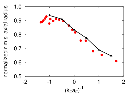
FIG. 2.: Comparison between experimental (dots) and theoretical (triangles) normalized root-mean square axial radius across the crossover regime. Experimental data are taken from Ref. 18. The values of $(k_{F}a_{F})^{-1}$ and of the non-interacting root-mean square axial radius used also for the experimental data are obtained with $N=2.3\times 10^{5}$.

The root-mean square axial radius has been normalized to its expression $\sqrt{E_{F}/(4m\omega_{z}^{2})}$ for non-interacting fermions. The values of $(k_{F}a_{F})^{-1}$ and of the non-interacting root-mean square axial radius (needed to compare the experimental data with our theoretical results) have been obtained with $N=2.3\times 10^{5}$, corresponding to the lower panel of Fig. 1. The agreement between theory and experiment is remarkably accurate even over this wide coupling range.

As mentioned already, comparison between a crossover theory and the experimental data is most compelling in the intermediate-coupling regime, due to the lack of a small parameter to control the many-body approximations [22] when the scattering length $a_{F}$ diverges. Special features further occur with a local theory at the unitarity limit $(k_{F}a_{F})^{-1}=0$. In particular, this limit corresponds in the isotropic case to the universal density profile (with $r=\mid{\mathbf{r}}\mid$)

$$n(r)=\frac{1}{3\pi^{2}(1+\beta)^{3/2}}[2m(E_{F}(1+\beta)^{1/2}-V(r))]^{3/2}$$ (6)

which depends on the single parameter $\beta$. This parameter was introduced experimentally in Ref. [23], and can be extracted theoretically from the ratio $\mu/E_{F}=1+\beta$ as obtained at the unitarity limit for the homogeneous system. For given values of the harmonic frequencies and of $\beta$, the density profile in Eq. (6) thus depends only on the total number of atoms $N$ via $E_{F}$.

Recent $T=0$ QMC simulations [12] have yielded the value $\beta=-0.56\pm 0.01$. Our theory gives $\beta=-0.545$, in excellent agreement with these simulations. By contrast, $T=0$ BCS mean field gives $\beta=-0.41$. Our theoretical value of $\beta$ is also fully consistent with recent experimental data, which yield the values $-0.68^{+0.13}_{-0.10}$ (Ref. [18]) and $-0.55\pm 0.10$ (Ref. [20]). The agreement between our theory and QMC simulations is further confirmed by comparing the values of the order parameter $\Delta$ at the unitarity limit for the homogeneous case. Our theory gives $\Delta/E_{F}=0.53$, while the QMC simulations of Ref. [12] provide the estimated value $\Delta/E_{F}=0.54$. It is then apparent that our crossover theory, which captures the essential physics on the two sides of the crossover, is also able to provide quantitatively accurate results in the intermediate-coupling regime, where no small parameter can be identified to control the many-body problem.

It is worth commenting that the number of atoms $N=2.3\times 10^{5}$, utilized by our calculations in the lower panel of Fig. 1 as well as in Fig. 2, was determined by equating the experimental value for the root-mean square axial radius at the unitarity limit given in Ref. [18], to the corresponding value obtained from the universal profile of Eq. (6) with $\beta$ taken from the QMC simulations of Ref. [12]. We have already seen from Fig. 1 (lower panel) and Fig. 2 that this value of $N$ makes the agreement between our theory and the experimental data remarkably good. This value of $N$ also improves considerably the agreement between the experimental value ($130nK$) as given in Ref. [18] for the bosonic chemical potential $\mu_{B}$ deep in the bosonic regime, and the corresponding theoretical estimate ($125nK$) obtained from the Gross-Pitaevskii theory [10] with the value $a_{B}=0.6a_{F}$ for the dimer-dimer scattering length $a_{B}$ [24]. If one would instead take $N=4.0\times 10^{5}$ (as in the upper panel of Fig. 1), a larger value ($155nK$) would result for the theoretical estimate of $\mu_{B}$.

In the present approach, the system of fermions maps in strong coupling onto a system of composite bosons (dimers), which are described by the Bogoliubov theory with a dimer-dimer scattering length $a_{B}/a_{F}=2$. This value corresponds to the Born approximation for the dimer-dimer scattering [25]. It has been shown [25] that inclusion of higher-order dimer-dimer scattering processes within the many-body diagrammatic theory decreases this value to $a_{B}/a_{F}=0.75$. A scattering approach to the four-fermion problem [24] has given instead the value $a_{B}/a_{F}=0.6$ quoted above. The difference between the values $0.75$ and $0.6$ originates from additional diagrams which were not considered in Ref. [25] albeit they survive in the zero-density limit. It is interesting that the difference between the values $2$ and $0.6-0.75$ can be appreciated, by analyzing the experimental results for the low-temperature axial density profile reported in Fig. 1(b) of Ref. [18] deep in the BEC region (corresponding to $(k_{F}a_{F})^{-1}=5.44$). Figure 3 compares the experimental results (dots) directly with the predictions of the Bogoliubov theory, obtained with the alternative values $a_{B}/a_{F}=2$ (dash-dotted line), $a_{B}/a_{F}=0.75$ (dashed line), and $a_{B}/a_{F}=0.6$ (full line). It is evident from this figure that a correct treatment of the dimer-dimer scattering improves the comparison with experimental data in this extreme BEC limit, where the dimer-dimer scattering length is the only relevant interaction parameter.

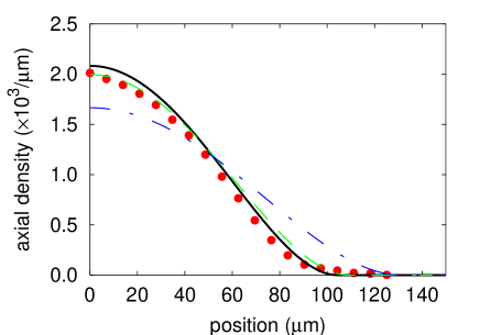
FIG. 3.: Comparison between experimental results for the axial density profile (dots) and the predictions of Bogoliubov theory, obtained with $a_{B}/a_{F}=2$ (dash-dotted line), $a_{B}/a_{F}=0.75$ (dashed line), and $a_{B}/a_{F}=0.6$ (full line). Experimental data were obtained in Ref. 18 deep in the BEC region, corresponding to $(k_{F}a_{F})^{-1}=5.44$ when $N=2.3\times 10^{5}$.

The analysis of the many-body diagrams made in Ref. [25] suggests, however, that inclusion of diagrams beyond the Born approximation for the dimer-dimer scattering should become immaterial when approaching the crossover region, as these diagrams correspond to high-order pairing-fluctuation processes of the Fermi system.

We comment finally that in our approach we have not introduced independent bosonic entities besides the fermions. The fermions themselves bind, in fact, into composite bosons even at finite temperature and density, provided their mutual attraction is sufficiently strong. Correspondingly, the many-body problem contains the two-fermion bound state via an effective single-channel problem with scattering length $a_{F}$, which can be identified directly with the scattering length varied experimentally via the FF resonance. The excellent agreement with the experimental data shown above demonstrates that this single-channel treatment is appropriate to describe the BCS-BEC crossover for trapped ⁶Li Fermi atoms.

We are indebted to R. Grimm, J.E. Thomas, and K. Levin for discussions, and to R. Grimm for providing us with the data files of the figures in Ref. [18]. This work was partially supported by the Italian MIUR (contract Cofin-2003 “Complex Systems and Many-Body Problems”).

REFERENCES

- [1] D.M. Eagles, Phys. Rev. 186, 456 (1969).
- [2] A.J. Leggett, in Modern Trends in the Theory of Condensed Matter, edited by A. Pekalski and R. Przystawa, Lecture Notes in Physics Vol.115 (Springer-Verlag, Berlin, 1980), p.13.
- [3] P. Nozières and S. Schmitt-Rink, J. Low. Temp. Phys. 59, 195 (1985).
- [4] C.W. Lai, J. Zoch. A.C. Gossard, and D.S. Chemla, Science 303, 503 (2004), and references quoted therein.
- [5] M. Baldo, U. Lombardo, and P. Schuck, Phys. Rev. C 52, 975 (1995).
- [6] See, e.g., V.M. Loktev, R.M. Quick, and S.G. Sharapov, Phys. Rep. 349, 1 (2001).
- [7] M. Greiner, C.A. Regal, and D.S. Jin, Nature 426, 537 (2003); S. Jochim, M. Bartenstein, A. Altmeyer, G. Hendl, S. Riedl, C. Chin, J. Hecker Denschlag, and R. Grimm, Science 302, 2101 (2003); M.W. Zwierlein, C.A. Stan, C.H. Schunck, S.M.F. Raupach, S. Gupta, Z. Hadzibabic, and W. Ketterle, Phys. Rev. Lett. 91, 250401 (2003); C.A. Regal, M. Greiner, and D.S. Jin, Phys. Rev. Lett. 92, 040403 (2004).
- [8] U. Fano, Nuovo Cimento 12, 156 (1935); Phys. Rev. 124, 1866 (1961); H. Feshbach, Ann. Phys. 19, 287 (1962); S. Inouye, M.R. Andrews, J. Stenger, H.-J. Miesner, D.M. Stamper-Kurn, and W. Ketterle, Nature 392, 151 (1998).
- [9] In contrast, for narrow resonances a bose-fermion model should be more appropriate. See, e.g., J.N. Milstein, S.J.J.M.F. Kokkelmans, and M.J. Holland, Phys. Rev. A 66, 043604 (2002); Y. Ohashi and A. Griffin, Phys. Rev. A 67, 033603 (2003).
- [10] F. Dalfovo, S. Giorgini, L.P. Pitaevskii, and S. Stringari, Rev. Mod. Phys. 71, 463 (1999).
- [11] Cf., e.g., A.L. Fetter and J.D. Walecka, Quantum Theory of Many-Particle Systems (McGraw-Hill, New York, 1971).
- [12] J. Carlson, S.-Y. Chang, V.R. Pandharipande, and K.E. Schmidt, Phys. Rev. Lett. 91, 050401 (2003).
- [13] P. Pieri, L. Pisani, and G.C. Strinati, Phys. Rev. Lett. 92, 110401 (2004).
- [14] A. Perali, P. Pieri, L. Pisani, and G.C. Strinati, Phys. Rev. Lett. (2004), in press.
- [15] V.N. Popov, Functional Integrals and Collective Excitations (Cambridge University Press, Cambridge, 1987).
- [16] J.R. Schrieffer, Theory of Superconductivity (W.A. Benjamin, New York, 1964), Chapter 8.
- [17] A. Perali, P. Pieri, and G.C. Strinati, Phys. Rev. A 68, 031601(R) (2003).
- [18] M. Bartenstein, A. Altmeyer, S. Riedl, S. Jochim, C. Chin, J. Hecker Denschlag, and R. Grimm, Phys. Rev. Lett. 92, 120401 (2004).
- [19] More recent data [20, 21] place the position of the resonance at about 820. With these data, the best estimated value of is about , to which there correspond the values -1.02, -0.55, and 0.32 for in Fig.1 (from left to right). Even with these new values of and the scattering length, we have verified that the agreement between the experimental and theoretical density profiles is very good.
- [20] T. Bourdel, L. Khaykovich, J. Cubizolles, J. Zhang, F. Chevy, M. Teichmann, L. Tarruell, S.J.J.M.F. Kokkelmans, and C. Salomon, cond-mat/0403091.
- [21] M.W. Zwierlein, C.A. Stan, C.H. Schunck, S.M.F. Raupach, A.J. Kerman, and W. Ketterle, cond-mat/0403049.
- [22] F. Dyson, Nature 427, 297 (2004).
- [23] K.M. O’Hara, S.L. Hemmer, M.E. Gehm, S.R. Granade, and J.E. Thomas, Science 298, 2179 (2002).
- [24] D. Petrov, C. Salomon, and G. Shlyapnikov, cond-mat/0309010.
- [25] P. Pieri and G.C. Strinati, Phys. Rev. B 61, 15370 (2000), and cond-mat/9811166.