Application of Kondo-lattice theory to the Mott-Hubbard metal-insulator crossover
in disordered cuprate oxide superconductors

Abstract

A theory of Kondo lattices is applied to the crossover between local-moment magnetism and itinerant-electron magnetism in the $t$-$J$ model on a quasi-two dimensional lattice. The Kondo temperature $T_{K}$ is defined as a characteristic temperature or energy scale of local quantum spin fluctuations. Magnetism with $T_{N}\gg T_{K}$, where $T_{N}$ is the Néel temperature, is characterized as local-moment one, while magnetism with $T_{N}\ll T_{K}$ is characterized as itinerant-electron one. The Kondo temperature, which also gives a measure of the strength of the quenching of magnetic moments, is renormalized by the Fock term of the superexchange interaction. Because the renormalization depends on life-time widths $\gamma$ of quasiparticles in such a way that $T_{K}$ is higher for smaller $\gamma$, $T_{N}$ can be controlled by disorder. The asymmetry of $T_{N}$ between electron-doped and hole-doped cuprates must mainly arise from that of disorder; an almost symmetric behavior of $T_{N}$ must be restored if we can prepare hole-doped and electron-doped cuprates with similar degree of disorder to each other. Because effective disorder is enhanced by magnetic fields in Kondo lattices, antiferromagnetic ordering must be induced by magnetic fields in cuprates that exhibit large magnetoresistance.

I Introduction

The discoverybednorz in 1986 of high transition-temperature (high-$T_{c}$) superconductivity in cuprate oxides has revived intensive and extensive studies on strong electron correlations because it occurs in the vicinity of the Mott-Hubbard metal-insulator transition or crossover. Cuprates with no dopings are Mott-Hubbard insulators, which exhibit antiferromagnetism at low temperatures. When electrons or holes are doped, they show the metal-insulator crossover. However, the crossover is asymmetric between electron-doped and hole-doped cuprates;asymmetric the insulating and antiferromagnetic phase is much wider as a function of dopings in electron-doped cuprates than it is in hole-doped cuprates. Because superconductivity appears in a metallic phase adjacent to the insulating phase, clarifying what causes the asymmetry is one of the most important issues to settle the mechanism of high-$T_{c}$ superconductivity itself among various proposals.

In 1963, three distinguished theories on electron correlations in a single-band model, which is now called the Hubbard model, were published by Kanamori,Kanamori Hubbard,Hubbard and Gutzwiller.Gutzwiller Two theories among them are directly related with the transition or crossover. According to Hubbard’s theory,Hubbard the band splits into two subbands called the lower and upper Hubbard bands. According to Gutzwiller’s theory,Gutzwiller with the help of the Fermi-liquid theory,Luttinger1 ; Luttinger2 a narrow quasiparticle band appears on the chemical potential; we call it Gutzwiller’s band in this paper. When we take both of them, we can argue that the density of states must be of a three-peak structure, Gutzwiller’s band on the chemical potential between the lower and upper Hubbard bands. This speculation was confirmed in a previous paper.OhkawaSlave The Mott-Hubbard splitting occurs in both metallic and insulating phases as long as the onsite repulsion $U$ is large enough, and Gutzwiller’s band is responsible for metallic behaviors. Then, we can argue that a metal with almost half filling can become an insulator only when a gap opens in Gutzwiller’s band or that it can behave as an insulator when life-time widths of Gutzwiller’s quasiparticles are so large that they can play no significant role.

Brinkman and RiceBrinkman considered the transition at $T=0$ K and the just half filling as a function of $U$ in Gutzwiller’s approximation.Gutzwiller They showed that the effective mass $m^{*}$ and the static homogeneous susceptibility $\chi_{s}(0,{\bf q}\rightarrow 0)$ diverge at a critical $U_{c}$. Their result implies that the ground state for $U>U_{c}$ must be a Mott-Hubbard insulator and the metal-insulator transition is of second order. In general, an order parameter appears in a second-order transition. However, there is no evidence that any order parameter appears in this transition. The absence of any order parameter contradicts the opening of gaps. The transition is caused by the disappearance of Gutzwiller’s band; the divergence of $m^{*}$ is one of its consequences. It is interesting to examine beyond Gutzwiller’s approximation, within the Hilbert subspace restricted within paramagnetic states, whether a hidden order parameter exists, whether the critical $U_{c}$ is finite or infinite, and whether the transition turns out to a crossover. It is also interesting to examine of which order the transition is, second order, first order, or crossover, at non-zero temperatures, where itinerant electrons and holes are thermally excited across the Mott-Hubbard gap.

It is also an interesting issue how the transition or crossover occurs as a function of electron or dopant concentrations. Once holes or electrons are doped into the Mott-Hubbard insulator that is just half filled, it must become a metal; unless a gap opens in Gutzwiller’s band, there is no reason why doped hole or electrons are localized in a periodic system. No metal-insulator transition can occur at nonzero concentrations of dopants even if $U$ is infinitely large. For the just half filling, on the other hand, a system with $U>U_{c}$ is the Mott-Hubbard insulator at $T=0$ K; $U_{c}$ may be finite or infinite. If $U_{c}$ is infinite, the point at $U=+\infty$ and the just half filling is a singular point in the phase-diagram plane of $U$ and electron concentrations; if $U_{c}$ is finite, the line on $U>U_{c}$ and the just half filling is a singular line. At $T=0$ K, a system is an insulator only at the singular point or on the singular line while it is a metal in the other whole region. However, either of these phase diagrams is totally different from observed ones. For example, cuprates with small amount of dopants are Mott-Hubbard insulators. When enough holes or electrons are doped, the insulators become paramagnetic metals. At low temperatures, they exhibit antiferromagnetism in insulating phases and superconductivity in metallic phases. The metal-insulator crossover in cuprates must be closely related with the disappearance of antiferromagnetic gaps in Gutzwiller’s band. It must also be closely related with the crossover between local-moment magnetism and itinerant-electron magnetism.

Not only Hubbard’sHubbard and Gutzwiller’sGutzwiller theories but also the previous theoryOhkawaSlave are within the single-site approximation (SSA). Their validity tells that local fluctuations are responsible for the three-peak structure. Local fluctuations are rigorously considered in one of the best SSA’s.comSSA Such an SSA is reduced to solving the Anderson model,Mapping which is one of the simplest effective Hamiltonians for the Kondo problem. The Kondo problem has already been solved.singlet ; poorman ; Wilson ; Nozieres ; Yamada ; Yosida One of the most essential physics involved in the Kondo problem is that a magnetic moment is quenched by local quantum spin fluctuations so that the ground states is a singletsinglet or a normal Fermi liquid.Wilson ; Nozieres The Kondo temperature $T_{K}$ is defined as a temperature or energy scale of local quantum spin fluctuations; it is also a measure of the strength of the quenching of magnetic moments. The so called Abrikosov-Suhl or Kondo peak between two sub-peaks corresponds to Gutzwiller’s band between the lower and upper Hubbard bands. Their peak-width or bandwidth is about $4k_{B}T_{K}$, with $k_{B}$ the Boltzmann constant.

On the basis of the mapping to the Kondo problem, we argue that a strongly correlated electron system on a lattice must show a metal-insulator crossover as a function of $T$: It is a nondegenerate Fermi liquid at $T\gg T_{K}$ because local thermal spin fluctuations are dominant, while it is a Landau’s normal Fermi liquid at $T\ll T_{K}$ because local quantum spin fluctuations are dominant and magnetic moments are quenched by them. Local-moment magnetism occurs at $T\gg T_{K}$, while itinerant-electron magnetism occurs at $T\ll T_{K}$; superconductivity can occur only at $T\ll T_{K}$, that is, in the region of itinerant electrons. The crossover implies that the coherence or incoherence of quasiparticles plays a crucial role in the metal-insulator crossover. The coherence is destroyed by not only thermal fluctuations but also disorder. Denote the life-time width of quasiparticles by $\gamma$. When $k_{B}T$ or $\gamma$ is larger than Gutzwiller’s bandwidth $W^{*}\simeq 4k_{B}T_{K}$ such as $k_{B}T\gtrsim W^{*}$ or $\gamma\gtrsim W^{*}$, Gutzwiller’s quasiparticles are never well-defined and they can never play a significant role; the system behaves as an insulator. When $k_{B}T\ll W^{*}$ and $\gamma\ll W^{*}$, on the other hand, they are well-defined and they can play a role; the system behaves as a metal. Disorder can play a significant role in the Mott-Hubbard metal-insulator transition or crossover.

A theory of Kondo lattices is formulated in such a way that an unperturbed state is constructed in one of the best SSA’scomSSA and intersite terms are perturbatively considered. It has already been applied to not only typical issues on electron correlations such as the Curie-Weiss law of itinerant-electron magnets,ohkawaCW ; miyai ferromagnetism induced by magnetic fields or metamagnetism,Satoh and itinerant-electron antiferromagnetism and ferromagnetism,ohkawaCW ; antiferromagnetism ; ferromagnetism but also high-$T_{c}$ superconductivity, the mechanism of superconductivity,OhkawaSC1 ; OhkawaSC2 ; OhkawaSC3 the opening of pseudogaps,OhkawaPseudogap the softening of phonons,OhkawaEl-ph and kinks in the quasiparticle dispersion.OhkawaEl-ph Early papersOhkawa87SC-1 ; Ohkawa87SC-2 ; Ohkawa90SC-3 on $d\gamma$-wave high-$T_{c}$ superconductivity, including the earliest two onesOhkawa87SC-1 ; Ohkawa87SC-2 published in 1987, can also be regarded within the theoretical framework of Kondo lattices. One of the purposes of this paper is to apply the theory of Kondo lattices to the crossover between local-moment magnetism and itinerant-electron magnetism. The other purpose is to show that the asymmetry of the Néel temperature $T_{N}$ between electron-doped and hole-doped cuprates can arise from that of disorder. This paper is organized as follows: The theory of Kondo lattices is reviewed in Sec. II. Effects of the coherence of quasiparticles on $T_{N}$ is studied in Sec. III. The asymmetry of $T_{N}$ in cuprates is examined in Sec. IV. Conclusion is given in Sec. V. The selfenergy of quasiparticles in disordered Kondo lattices is studied in Appendix A. A possible mechanism for the deviation of the Abrikosov-Gorkov theoryabrikoso-gorkov is studied in Appendix B.

II Kondo-lattice theory

II.1 Renormalized SSA

We consider the $t$-$J$ or $t$-$t^{\prime}$-$J$ model on a simple square lattices with lattice constant $a$:exchByOhkawa

$${\cal H} = -t\sum_{\left<ij\right>\sigma}a_{i\sigma}^{\dagger}a_{j\sigma}-t^{\prime}\sum_{\left<ij\right>^{\prime}\sigma}a_{i\sigma}^{\dagger}a_{j\sigma}$$ (1)

$$\quad-\frac{1}{2}J\sum_{\left<ij\right>}({\bf S}_{i}\cdot{\bf S}_{j})+U_{\infty}\sum_{i}n_{i\uparrow}n_{i\downarrow},\quad$$

with $t$ the transfer integral between nearest neighbors $\left<ij\right>$, $t^{\prime}$ between next-nearest neighbors $\left<ij\right>^{\prime}$, ${\bf S}_{i}=\sum_{\alpha\beta}\frac{1}{2}\left(\sigma_{x}^{\alpha\beta},\sigma_{y}^{\alpha\beta},\sigma_{z}^{\alpha\beta}\right)a_{i\alpha}^{\dagger}a_{i\beta}$, with $\sigma_{x}$, $\sigma_{y}$, and $\sigma_{z}$ being the Pauli matrices, and $n_{i\sigma}=a_{i\sigma}^{\dagger}a_{i\sigma}$. Because we are interested in cuprates, we assume that $t>0$ and the superexchange interaction is nonzero only between nearest neighbors and is antiferromagnetic;

$$J/|t|=-0.3.$$ (2)

Infinitely large onsite repulsion, $U_{\infty}/|t|\rightarrow+\infty$, is introduced in order to exclude doubly occupied sites. Effects of disorder and weak three dimensionality are phenomenologically considered in this paper.

The $t$-$J$ model (1) can only treat less-than-half fillings. When we take the hole picture, we can also treat more-than-half fillings with the model (1) with the signs of $t$ and $t^{\prime}$ reversed. We consider two models: a symmetric one with $t^{\prime}=0$, and an asymmetric one with $t^{\prime}/t\simeq-0.3$, whose precise definition is made below. In the symmetric model, physical properties are symmetric between less-than-half and more-than-half fillings.

We follow the previous paperOhkawaPseudogap to treat the infinitely large $U_{\infty}$. The single-particle selfenergy $\Sigma_{\sigma}(i\varepsilon_{n},{\bf k})$ is divided into a single-site term $\tilde{\Sigma}_{\sigma}(i\varepsilon_{n})$, an energy-independent multisite term $\Delta\Sigma_{\sigma}({\bf k})$, and an energy-dependent multisite term $\Delta\Sigma_{\sigma}(i\varepsilon_{n},{\bf k})$: $\Sigma_{\sigma}(i\varepsilon_{n},{\bf k})=\tilde{\Sigma}_{\sigma}(i\varepsilon_{n})+\Delta\Sigma_{\sigma}({\bf k})+\Delta\Sigma_{\sigma}(i\varepsilon_{n},{\bf k})$. As is discussed below, $\Delta\Sigma_{\sigma}({\bf k})$ is the Fock term due to $J$. First, we take a renormalized SSA, which includes not only $\tilde{\Sigma}_{\sigma}(i\varepsilon_{n})$ but also $\Delta\Sigma_{\sigma}({\bf k})$. The SSA is reduced to solving a mapped Anderson model. The mapping condition is simple:Mapping The onsite repulsion of the Anderson model should be $U_{\infty}$, and other parameters should be determined to satisfy

$$\tilde{G}_{\sigma}(i\varepsilon_{n})\!=\!\frac{1}{N}\sum_{\bf k}G_{\sigma}^{(0)}(i\varepsilon_{n},{\bf k}),$$ (3)

with $\tilde{G}_{\sigma}(i\varepsilon_{n})$ the Green function of the Anderson model, and $G_{\sigma}^{(0)}(i\varepsilon_{n},{\bf k})=1/[i\varepsilon_{n}\!\!+\!\mu\!-\!E({\bf k})\!-\!\tilde{\Sigma}_{\sigma}(i\varepsilon_{n})\!-\!\Delta\Sigma_{\sigma}({\bf k})]$. Here, $\mu$ is the chemical potential, and

$$E({\bf k})=-2t\eta_{1s}({\bf k})-2t^{\prime}\eta_{2s}({\bf k}),$$ (4)

with

$$\eta_{1s}({\bf k}) = \cos(k_{x}a)+\cos(k_{y}a),$$ (5a)

$$\eta_{2s}({\bf k}) = 2\cos(k_{x}a)\cos(k_{y}a),$$ (5b)

is the dispersion relation of unrenormalized electrons. The single-site term $\tilde{\Sigma}_{\sigma}(i\varepsilon_{n})$ is given by the selfenergy of the Anderson model. It is expanded as

$$\tilde{\Sigma}_{\sigma}(i\varepsilon_{n})=\tilde{\Sigma}(0)\!+\!(1\!-\!\tilde{\phi}_{\gamma})i\varepsilon_{n}\!+\!\sum_{\sigma^{\prime}}(1\!-\!\tilde{\phi}_{\sigma\sigma^{\prime}})\Delta\mu_{\sigma^{\prime}}+\cdots,$$ (6)

with $\Delta\mu_{\sigma}$ an infinitesimally small spin-dependent chemical potential shift. Note that $\tilde{\phi}_{\gamma}=\tilde{\phi}_{\sigma\sigma}$. The Wilson ratio is defined by $\tilde{W}_{s}=\tilde{\phi}_{s}/\tilde{\phi}_{\gamma}$, with $\tilde{\phi}_{s}=\tilde{\phi}_{\sigma\sigma}-\tilde{\phi}_{\sigma-\sigma}$. For almost half fillings, charge fluctuations are suppressed so that $\tilde{\phi}_{c}=\tilde{\phi}_{\sigma\sigma}+\tilde{\phi}_{\sigma-\sigma}\ll 1$. For such fillings, $\tilde{\phi}_{\gamma}\gg 1$ so that $\tilde{\phi}_{s}\simeq 2\tilde{\phi}_{\gamma}$ or $\tilde{W}_{s}\simeq 2$.

The Green function in the renormalized SSA is divided into coherent and incoherent parts: $G_{\sigma}^{(0)}(i\varepsilon_{n},{\bf k})=(1/\tilde{\phi}_{\gamma})g_{\sigma}^{(0)}(i\varepsilon_{n},{\bf k})\!+\!\mbox{(incoherent part)}$, with

$$g_{\sigma}^{(0)}(i\varepsilon_{n},{\bf k})=\frac{1}{i\varepsilon_{n}+\mu^{*}-\xi({\bf k})+i\gamma\mbox{sign}(\varepsilon_{n})},$$ (7)

where $\mu^{*}=(\mu-\tilde{\Sigma}_{0})/\tilde{\phi}_{\gamma}$ is an effective chemical potential, $\xi({\bf k})=[E({\bf k})+\Delta\Sigma({\bf k})]/\tilde{\phi}_{\gamma}$ is the dispersion relation of quasiparticles in the renormalized SSA, and $\mbox{sign}(\varepsilon_{n})=\varepsilon_{n}/|\varepsilon_{n}|$; the incoherent part describes the lower and upper Hubbard bands. We introduce a phenomenological life-time width $\gamma$, which is partly due to disorder and partly due to many-body effects. Although $\gamma$ depends on energies in general even if it is due to disorder, as is discussed in Appendix A, its energy dependence is ignored.ComGamma Effects of life-time widths or the coherence of quasiparticles on the crossover between local-moment magnetism and itinerant-electron magnetism can be, at least qualitatively, examined even in this simplified scheme.

According to the Fermi-surface sum rule,Luttinger1 ; Luttinger2 the number of electrons is given by that of quasiparticles; the density or the number of electrons per site for $T/T_{K}\rightarrow+0$ and $\gamma/k_{B}T_{K}\rightarrow+0$ is given by

$$n = 2\frac{k_{B}T}{N}\sum_{\varepsilon_{n}{\bf k}}e^{i\varepsilon_{n}0^{+}}g_{\sigma}(i\varepsilon_{n},{\bf k})$$ (8)

$$= 2\!\!\int\!\!d\varepsilon\rho_{\gamma\rightarrow 0}(\varepsilon)f_{\gamma}(\varepsilon\!-\!\mu^{*})$$

$$= 2\!\!\int\!d\varepsilon\rho_{\gamma}(\varepsilon)f_{\gamma=0}(\varepsilon\!-\!\mu^{*}),$$

with

$$\rho_{\gamma}(\varepsilon)=\frac{1}{\pi N}\sum_{\bf k}\frac{\gamma}{\left[\varepsilon-\xi({\bf k})\right]^{2}+\gamma^{2}},\qquad$$ (9)

$$f_{\gamma}(\varepsilon)=\frac{1}{2}+\frac{1}{\pi}\mbox{Im}\left[\psi\left(\frac{1}{2}+\frac{\gamma-i\varepsilon}{2\pi k_{B}T}\right)\right],$$ (10)

with $\psi(z)$ the di-gamma function. Note that $f_{\gamma=0}(\varepsilon)=1/\left[e^{\varepsilon/k_{B}T}+1\right]$. We assume Eq. (8) even for nonzero $T$ and $\gamma$. The parameter $\tilde{\Sigma}_{0}$ or $\mu^{*}$ can be determined from Eq. (8) as a function of $n$.

II.2 Intersite exchange interaction

Denote susceptibilities of the Anderson and the $t$-$J$ models, which do not include the factor $\frac{1}{4}g^{2}\mu_{B}^{2}$ with $g$ being the $g$ factor and $\mu_{B}$ the Bohr magneton, by $\tilde{\chi}_{s}(i\omega_{l})$ and $\chi_{s}(i\omega_{l},{\bf q})$, respectively. In Kondo lattices, local spin fluctuations at different sites interact with each other by an exchange interaction. Following this physical picture, we define an exchange interaction $I_{s}(i\omega_{l},{\bf q})$ by

$$\chi_{s}(i\omega_{l},{\bf q})=\frac{\tilde{\chi}_{s}(i\omega_{l})}{1-\mbox{$\frac{1}{4}$}I_{s}(i\omega_{l},{\bf q})\tilde{\chi}_{s}(i\omega_{l})}.$$ (11)

Following the previous paper,OhkawaPseudogap we obtain

$$I_{s}(i\omega_{l},{\bf q})=J({\bf q})+2U_{\infty}^{2}\Delta\pi_{s}(i\omega_{l},{\bf q}),$$ (12)

with $\Delta\pi_{s}(i\omega_{l},{\bf q})$ the multi-site part of the irreducible polarization function in spin channels; $2U_{\infty}^{2}\Delta\pi_{s}(i\omega_{l},{\bf q})$ is examined in Secs. III.2 and III.3.

When the Ward relation ward is made use of, the irreducible single-site three-point vertex function in spin channels, $\tilde{\lambda}_{s}(i\varepsilon_{n},i\varepsilon_{n}\!+\!i\omega_{l};i\omega_{l})$, is given by

$$U_{\infty}\tilde{\lambda}_{s}(i\varepsilon_{n},i\varepsilon_{n}+i\omega_{l};i\omega_{l})=2\tilde{\phi}_{s}/\tilde{\chi}_{s}(i\omega_{l}),$$ (13)

for $|\varepsilon_{n}|\rightarrow+0$ and $|\omega_{l}|\rightarrow+0$. We approximately use Eq. (13) for $|\varepsilon_{n}|\lesssim 2k_{B}T_{K}$ and $|\omega_{l}|\lesssim 2k_{B}T_{K}$, with $T_{K}$ the Kondo temperature defined by

$$k_{B}T_{K}=\left[1/\tilde{\chi}_{s}(0)\right]_{T\rightarrow 0}.$$ (14)

An exchange interaction mediated by spin fluctuations is calculated in such a way that

$$\frac{1}{4}\!\left[2\tilde{\phi}_{s}/\tilde{\chi}_{s}(i\omega_{l})\right]^{2}F_{s}(i\omega_{l},{\bf q})=\tilde{\phi}_{s}^{2}\frac{1}{4}I_{s}^{*}(i\omega_{l},{\bf q}),$$ (15)

with

$$F_{s}(i\omega_{l},{\bf q}) = \chi_{s}(i\omega_{l},{\bf q})-\tilde{\chi}_{s}(i\omega_{l}),$$ (16)

$$\frac{1}{4}I_{s}^{*}(i\omega_{l},{\bf q}) = \frac{\frac{1}{4}I_{s}(i\omega_{l},{\bf q})}{1-\frac{1}{4}I_{s}(i\omega_{l},{\bf q})\tilde{\chi}_{s}(i\omega_{l})}.$$ (17)

The single-site term is subtracted in $F_{s}(i\omega_{l},{\bf q})$ because it is considered in SSA.

Because of these equations, we call $I_{s}(i\omega_{l},{\bf q})$ a bare exchange interaction, $I_{s}^{*}(i\omega_{l},{\bf q})$ an enhanced one, and $\tilde{\phi}_{s}$ an effective three-point vertex function in spin channels. Because the spin space is isotropic, the interaction in the transversal channels is also given by these equations. Intersite effects can be perturbatively considered in terms of $I_{s}(i\omega_{l},{\bf q})$, $I_{s}^{*}(i\omega_{l},{\bf q})$ or $F_{s}(i\omega_{l},{\bf q})$ depending on each situation.CommentSC

       

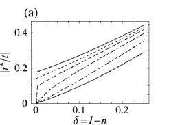
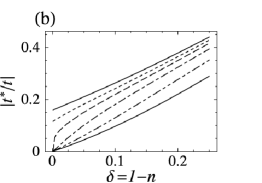
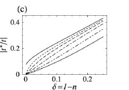
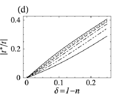
Figure 1: Renormalized transfer integrals $t^{*}$ of quasiparticles in the unperturbed state of the symmetric model: (a) $k_{B}T/|t|=0.02$, (b) $k_{B}T/|t|=0.1$, (c) $k_{B}T/|t|=0.2$, and (d) $k_{B}T/|t|=0.4$. In each figure, topmost solid, dotted, broken, dot-broken, and two-dot-broken lines show results for $\gamma/|t|=0.01$, 0.1, 0.2, and 0.4, respectively. For comparison, $1/\tilde{\phi}_{\gamma}$ is also shown by a bottom solid line.

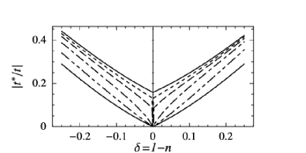
Figure 2: $t^{*}$ of the asymmetric model for $k_{B}T/|t|=0.02$. See also the caption of Fig. 1; this figure corresponds to Fig. 1(a) for the symmetric model.

II.3 Fock term of the superexchange interaction

Note that $\lim_{\omega_{l}\rightarrow+\infty}I_{s}^{*}(i\omega_{l},{\bf q})=J({\bf q})$. We consider the multisite selfenergy correction due to high-energy spin excitations or due to the superexchange interaction $J({\bf q})$. The Fock term of $J({\bf q})$ gives a selfenergy correction independent of energies:exchByOhkawa

$$\Delta\Sigma_{\sigma}({\bf k})\!=\!\frac{3}{4}\tilde{\phi}_{s}^{2}\frac{k_{B}T}{N}\!\!\sum_{\varepsilon_{n}{\bf p}}\!J({\bf k}\!-\!{\bf p})e^{i\varepsilon_{m}0^{+}}\!G_{\sigma}(i\varepsilon_{n},{\bf p}).$$ (18)

The factor 3 appears because of three spin channels. When only the coherent part is considered,

$$\frac{1}{\tilde{\phi}_{\gamma}}\Delta\Sigma_{\sigma}({\bf k})=\frac{3}{4}\tilde{W}_{s}^{2}J\Xi\eta_{1s}({\bf k}),$$ (19)

with

$$\Xi=\frac{1}{N}\sum_{\bf k}\eta_{s}({\bf k})f_{\gamma}\left[\xi({\bf k})-\mu^{*}\right].$$ (20)

The dispersion relation of quasiparticles is given by

$$\xi({\bf k})=-2t^{*}\eta_{1s}({\bf k})-2t_{2}^{*}\eta_{2s}({\bf k})$$ (21)

in the renormalized SSA. The effective transfer integral $t^{*}$ should be selfconsistently determined to satisfy

$$2t^{*}=\frac{2t}{\tilde{\phi}_{\gamma}}-\frac{3}{4}\tilde{W}_{s}^{2}J\Xi,$$ (22)

while $t_{2}^{*}$ is simply given by $t_{2}^{*}=t^{\prime}/\tilde{\phi}_{\gamma}$.

For the symmetric model, $t^{\prime}=0$ so that $t_{2}^{*}=0$. In order to examine how crucial role the shape of the Fermi surface plays in the asymmetry, we consider a phenomenological asymmetric model with

$$t_{2}^{*}/t^{*}=-0.3.$$ (23)

Expansion parameters $\tilde{\phi}_{\gamma}$ and $\tilde{\phi}_{s}$ are given by those of the mapped Anderson model, which should be selfconsistently determined to satisfy Eqs. (3) and (22). However, we approximately use those for the Anderson model with a constant hybridization energy. According to Appendix of the previous paper,ferromagnetism

$$\tilde{\phi}_{\gamma}=\frac{1}{2}\left(\frac{1}{|\delta|}+|\delta|\right)\frac{\displaystyle\left(\pi/2\right)^{2}(1-|\delta|)^{2}}{\displaystyle\cos^{2}\!\left(\pi\delta/2\right)},$$ (24)

$$\tilde{\phi}_{s}=\frac{1}{|\delta|}\frac{\displaystyle\left(\pi/2\right)^{2}(1-|\delta|)^{2}}{\displaystyle\cos^{2}\!\left(\pi\delta/2\right)},$$ (25)

where

$$\delta=1-n$$ (26)

is the concentration of dopants, holes ($\delta>0$) or electrons ($\delta<0$). These are consistent with Gutzwiller’s theory.Gutzwiller

Figures 1 and 2 show $t^{*}$ of the symmetric and asymmetric models, respectively, as a function of $\delta$. It is interesting that $t^{*}$ is nonzero even for $\delta\rightarrow 0$ if life-time widths $\gamma$ are small enough and temperatures $T$ are low enough. For the symmetric model ($t_{2}^{*}=0$), Eq. (20) can be analytically calculated for $T=0$ K, $\gamma=0$ and $\delta=0$ $(\mu^{*}=0)$ so that $\Xi=4/\pi^{2}$. Then, $\left[t^{*}/t\right]_{\delta\rightarrow 0}\rightarrow-3\tilde{W}_{s}^{2}(J/t)/2\pi^{2}=0.18$ for the symmetric model. If $\gamma$ are large enough or $T$ are high enough, on the other hand, $\Xi$ and $t^{*}$ vanish for $\delta\rightarrow 0$.

Figure 3 shows physical properties of the unperturbed state of the symmetric model: $\rho_{\gamma}(\varepsilon)$, $\mu^{*}$ as a function of $n$, $n$ as a function of $\mu^{*}$, and Fermi surfaces for various $n$. Physical properties of the unperturbed state of the asymmetric model can be found in Fig. 2 of Ref. OhkawaPseudogap, .

     

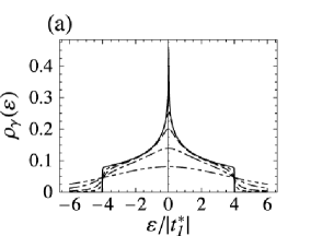
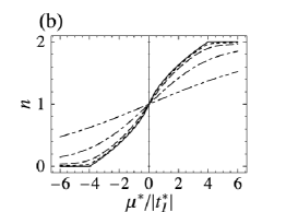
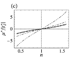
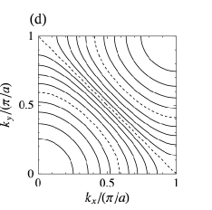
Figure 3: Single-particle properties of the unperturbed state of the symmetric model. (a) Density of states for quasiparticles $\rho_{\gamma}(\varepsilon)$, (b) effective chemical potentials, $\mu^{*}$, as functions of carrier concentrations $n$, and (c) $n$ as functions of $\mu^{*}$. In these three figures, solid, dotted, broken, dot-broken, and two-dot-broken lines show results for $\gamma/|t^{*}|=10^{-3}$, 0.1, 0.3, 1, and 3, respectively. Note that the solid and dotted lines are the almost same as each other. (d) Fermi surfaces for $k_{B}T=0$, $\gamma=0$, and 19 electron concentrations such as $n=0.1\times i$, with $1\leq i\leq 19$ being an integer. Dotted lines show Fermi surfaces for $n=$0.5, 1.0, and 1.5. Single-particle properties of the asymmetric model can be found in Fig. 2 of Ref. OhkawaPseudogap, .

III Suppression of the Néel temperature by spin fluctuations

III.1 Renormalization of the Kondo temperature

According to Eq. (11), the Néel temperature $T_{N}$ is determined by

$$1-\frac{1}{4}I_{s}(0,{\bf Q})\tilde{\chi}_{s}(0)=0.$$ (27)

Here, Q is an ordering wave number to be determined.

The local susceptibility $\tilde{\chi}_{s}(0)$ is almost constant at $T\ll T_{K}$, while it obeys the Curie law at high temperatures such as $\tilde{\chi}_{s}(0)=n/k_{B}T$ at $T\gg T_{K}$. In this paper, we use an interpolation between the two limits:

$$\tilde{\chi}_{s}(0)=\frac{n}{\displaystyle k_{B}\sqrt{n^{2}T_{K}^{2}+T^{2}}},$$ (28)

with $T_{K}$ defined by Eq. (14).

The renormalization of $t^{*}$ by the Fock term is nothing but the renormalization of local quantum spin fluctuations or their energy scale $k_{B}T_{K}$ by the superexchange interaction. According to Eq. (14) together with the Fermi-liquid relationYamada ; Yosida and the mapping condition (3), the static susceptibility or $k_{B}T_{K}$ is given by

$$\left[\tilde{\chi}_{s}(0)\right]_{T=0\mbox{~{}\scriptsize K}} = \frac{1}{k_{B}T_{K}}=2\tilde{W}_{s}\left[\rho_{\gamma}(\mu^{*})\right]_{\gamma\rightarrow 0},$$ (29)

in the absence of disorder. In disordered systems, the mapping conditions are different from site to site so that $T_{K}$ are also different from site to site. Such disorder in $T_{K}$ causes energy-dependent life-time width, as is studied in Appendix A. However, life-time widths due to the disorder in $T_{K}$ are small on the chemical potential in case of non-magnetic impurities. Then, a mean value of $T_{K}$ in disordered systems is approximately given by Eq. (29) with nonzero but small $\gamma$. It follows from Eq. (29) that

$$k_{B}T_{K}=\frac{|t^{*}|}{c_{T_{K}}}\frac{1}{2\tilde{W}_{s}},$$ (30)

with $c_{T_{K}}$ a numerical constant depending on $n$. As is shown in Fig. 3(a), $\rho_{\gamma}(\mu^{*})\simeq 0.15$ for $0.1\lesssim\gamma/|t^{*}|\lesssim 1$ and $0.05\lesssim|\delta|\lesssim 0.25$. We assume that $c_{T_{K}}$ is independent of $n$ for the sake of simplicity:

$$c_{T_{K}}=0.15.$$ (31)

We are only interested in physical properties that never drastically change when $c_{T_{K}}$ slightly changes.

III.2 Exchange interaction arising from the virtual exchange of pair excitations of quasiparticles

The first term of Eq. (12) is the superexchange interaction.exchByOhkawa The second term is the sum of an exchange interaction arising from that of pair excitations of quasiparticles, $J_{Q}(i\omega_{l},{\bf q})$, and the mode-mode coupling term, $-4\Lambda(i\omega_{l},{\bf q})$:

$$2U_{\infty}^{2}\Delta\pi_{s}(i\omega_{l},{\bf q})=J_{Q}(i\omega_{l},{\bf q})-4\Lambda(i\omega_{l},{\bf q}).$$ (32)

When higher-order terms in intersite effects are ignored,

$$J_{Q}(i\omega_{l},{\bf q})=4\left[\frac{\tilde{W}_{s}}{\tilde{\chi}_{s}(0)}\right]^{2}\left[P(i\omega_{l},{\bf q})-P_{0}(i\omega_{l})\right],$$ (33)

with

$$P(i\omega_{l},{\bf q})=\frac{k_{B}T}{N}\!\!\sum_{\varepsilon_{n}{\bf k}\sigma}\!g_{\sigma}^{(0)}(i\varepsilon_{n}\!+\!i\omega_{l},{\bf k}\!+\!{\bf q})g_{\sigma}^{(0)}(i\varepsilon_{n},{\bf k}).$$ (34)

The local contribution $P_{0}(i\omega_{l})=(1/N)\sum_{\bf q}P(i\omega_{l},{\bf q})$ is subtracted because it is considered in SSA. The static component is simply given by

$$P(0,{\bf q})=\frac{2}{N}\!\sum_{\bf k}\!\frac{f_{\gamma}\bigl{[}\xi({\bf k}\!+\!{\bf q})\!-\!\mu^{*}\bigr{]}\!-\!f_{\gamma}\bigl{[}\xi({\bf k})\!-\!\mu^{*}\bigr{]}}{\xi({\bf k})-\xi({\bf k}+{\bf q})-i0}.$$ (35)

Figures 4 and 5 show $[P(0,{\bf q})-P_{0}(0)]$ of the symmetric and asymmetric models. The polarization function is relatively larger in electron-doping cases than it is in hole-doping cases.

The magnitude of $J_{Q}(i\omega_{l},{\bf q})$ is proportional to $k_{B}T_{K}$ or the bandwidth of quasiparticles. According to previous papers,ohkawaCW ; miyai an almost $T$-linear dependence of $J_{Q}(+i0,{\bf q})$ at $T\ll T_{K}$ in a small region of ${\bf q}$, ${\bf q}\simeq 0$ for ferromagnets and ${\bf q}\simeq{\bf Q}$ for antiferromagnets, with ${\bf Q}$ being the nesting wavenumber, is responsible for the Curie-Weiss law of itinerant-electron magnets; the $T$-linear dependence of $1/\tilde{\chi}_{s}(0)$ at $T\gg T_{K}$ is responsible for the Curie-Weiss law of local-moment magnets. Magnetism with $T_{N}\gg T_{K}$ is characterized as local-moment one, while magnetism with $T_{N}\ll T_{K}$ is characterized as itinerant-electron one.

      

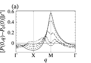
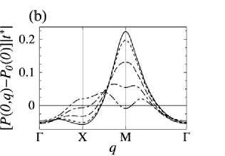
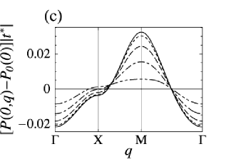
Figure 4: Static polarization function $[P(0,{\bf q})-P_{0}(0)]|t^{*}|$ of the symmetric model: (a) $k_{B}T/|t^{*}|=\gamma/|t^{*}|=0.1$, (b) $k_{B}T/|t^{*}|=\gamma/|t^{*}|=0.3$, and (c) $k_{B}T/|t^{*}|=\gamma/|t^{*}|=1$. Solid, dotted, broken, dot-broken, and double-dot-broken lines show results for $n\rightarrow 1$, $n=0.9$, 0.8, 0.7, and 0.6, respectively. Here, $\Gamma$, $X$ and $M$ stand for $(0,0)$, $(\pi/a,0)$ and $(\pi/a,\pi/a)$, respectively.

       

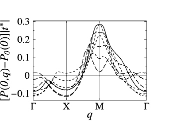
Figure 5: $[P(0,{\bf q})-P_{0}(0)]|t^{*}|$ of the asymmetric model: $k_{B}T/|t^{*}|=\gamma/|t^{*}|=0.1$. A solid line shows a result for $n\rightarrow 1$, dotted lines results of electron doping cases such as $n=1.1$, 1.2 and 1.3, and broken lines results for hole doping cases such as $n=0.9$, 0.8, and 0.7. In either doping case, the polarization function at $M$ point decreases with increasing concentrations of dopants $|\delta|=|1-n|$.

III.3 Mode-mode coupling terms

Following previous papers,miyai ; kawabata ; OhkawaModeMode we consider mode-mode coupling terms linear in intersite spin fluctuations $F_{s}(i\omega_{l},{\bf q})$ given by Eq. (16):

$$\Lambda(i\omega,{\bf q})=\Lambda_{L}(i\omega_{l})+\Lambda_{s}(i\omega_{l},{\bf q})+\Lambda_{v}(i\omega_{l},{\bf q}).$$ (36)

The first term $\Lambda_{L}(i\omega_{l})$ is a local mode-mode coupling term, which includes a single local four-point vertex function, as is shown in Fig. 4 of Ref. OhkawaModeMode, . Both of $\Lambda_{s}(i\omega_{l},{\bf q})$ and $\Lambda_{v}(i\omega_{l},{\bf q})$ are intersite mode-mode coupling terms, which include a single intersite four-point vertex function; a single $F(i\omega_{l},{\bf q})$ appears as the selfenergy correction to the single-particle Green function in $\Lambda_{s}(i\omega_{l},{\bf q})$ while it appears as a vertex correction to the polarization function in $\Lambda_{v}(i\omega_{l},{\bf q})$, as are shown in Figs. 3(a) and 3(b), respectively, of Ref. OhkawaModeMode, . Their static components are given by

$$\Lambda_{L}(0)=\frac{5}{2\tilde{\chi}_{s}(0)}\frac{k_{B}T}{N}\sum_{\omega_{l}{\bf q}}F_{s}(i\omega_{l},{\bf q}),$$ (37)

$$\Lambda_{s}(0,{\bf q}) = \frac{3}{\tilde{\chi}_{s}(0)}\frac{k_{B}T}{N}\sum_{\omega_{l},{\bf p}}B_{s}(i\omega_{l},{\bf p};{\bf q})$$ (38)

$$\times\left[F_{s}(i\omega_{l},{\bf q})-\frac{1}{4}J({\bf q})\tilde{\chi}_{s}^{2}(i\omega_{l})\right],$$

and

$$\Lambda_{v}(0,{\bf q})=-\frac{1}{2\tilde{\chi}_{s}(0)}\frac{k_{B}T}{N}\sum_{\omega_{l},{\bf p}}B_{v}(i\omega_{l},{\bf p};{\bf q})F_{s}(i\omega_{l},{\bf q}),$$ (39)

with

$$B_{s}(i\omega_{l},{\bf p};{\bf q}) = \frac{4\tilde{W}_{s}^{4}}{\tilde{\chi}_{s}^{3}(0)}k_{B}T\sum_{\varepsilon_{n}}\Biggl{\{}\frac{1}{N}\sum_{\bf k}g_{\sigma}^{(0)}(i\varepsilon_{n},{\bf k}-{\bf q})$$ (40)

$$\times\left[g_{\sigma}^{(0)}(i\varepsilon_{n},{\bf k})\right]^{2}g_{\sigma}^{(0)}(i\varepsilon_{n}+i\omega_{l},{\bf k}+{\bf p})$$

$$-\left[r_{\sigma}^{(0)}(i\varepsilon_{n})\right]^{3}r_{\sigma}^{(0)}(i\varepsilon_{n}+i\omega_{l})\Biggr{\}},$$

and

$$B_{v}(i\omega_{l},{\bf p};{\bf q}) = \frac{4\tilde{W}_{s}^{4}}{\tilde{\chi}_{s}^{3}(0)}k_{B}T\sum_{\varepsilon_{n}}\Biggl{\{}\frac{1}{N}\sum_{\bf k}g_{\sigma}^{(0)}(i\varepsilon_{n},{\bf k}+{\bf q})$$ (41)

$$\times g_{\sigma}^{(0)}(i\varepsilon_{n},{\bf k})g_{\sigma}^{(0)}(i\varepsilon_{n}+i\omega_{l},{\bf k}+{\bf q}+{\bf p})$$

$$\times g_{\sigma}^{(0)}(i\varepsilon_{n}+i\omega_{l},{\bf k}+{\bf p})$$

$$-\left[r_{\sigma}^{(0)}(i\varepsilon_{n})\right]^{2}\!\left[r_{\sigma}^{(0)}(i\varepsilon_{n}\!+\!i\omega_{l})\right]^{2}\Biggr{\}},$$

with

$$r_{\sigma}^{(0)}(i\varepsilon_{n})=\frac{1}{N}\sum_{\bf k}g_{\sigma}^{(0)}(i\varepsilon_{n},{\bf k}).$$ (42)

Because the selfenergy correction linear in $J({\bf q})$ is considered in Sec. II.3, $\frac{1}{4}J({\bf q})\tilde{\chi}_{s}^{2}(i\omega_{l})$ is subtracted in Eq. (38).

In this paper, weak three dimensionality in spin fluctuations is phenomenologically included. Because $J({\bf q})$ has its maximum value at ${\bf q}=(\pm\pi/a,\pm\pi/a)$ and the nesting vector of the Fermi surface in two dimensions is also close to ${\bf q}=(\pm\pi/a,\pm\pi/a)$ for almost half filling, we assume that the ordering wave number in three dimensions is

$${\bf Q}=(\pm\pi/a,\pm\pi/a,\pm Q_{z}),$$ (43)

with $Q_{z}$ depending on interlayer exchange interactions. On the phase boundary between paramagnetic and antiferromagnetic phases, where Eq. (27) is satisfied, the inverse of the susceptibility is expanded around ${\bf Q}$ and for small $\omega_{l}$ in such a way that

$$\left[1/\chi_{s}(i\omega_{l},{\bf Q}+{\bf q})\right]_{T=T_{N}}=A({\bf q})+\alpha_{\omega}|\omega_{l}|+\cdots,$$ (44)

with

$$A({\bf q})=\frac{1}{4}A_{\parallel}({\bf q}_{\parallel}a)^{2}+\frac{1}{4}A_{z}\left[(q_{z}-Q_{z})c\right]^{2}.$$ (45)

Here, $c$ is the lattice constant along the $z$ axis. Because $\chi_{s}(i\omega_{l},{\bf Q}+{\bf q})$ diverges in the limit of $|{\bf q}|\rightarrow 0$ and $\omega_{l}\rightarrow 0$ on the phase boundary,

$$B_{s}(0,-{\bf Q};{\bf Q}) = B_{v}(0,-{\bf Q};{\bf Q})$$ (46)

$$= \frac{4\tilde{W}_{s}^{4}}{\tilde{\chi}_{s}^{3}}k_{B}T\sum_{\varepsilon_{n}}\Biggl{\{}\frac{1}{N}\!\sum_{\bf k}\left[g_{\sigma}^{(0)}(i\varepsilon_{n},{\bf k}\!-\!{\bf Q})\right]^{2}$$

$$\times\left[g_{\sigma}^{(0)}(i\varepsilon_{n},{\bf k})\right]^{2}-\left[r_{\sigma}^{(0)}(i\varepsilon_{n})\right]^{4}\Biggr{\}},$$

can be approximately used for $B_{s}(i\omega_{l},{\bf p};{\bf q})$ in Eq. (38) and $B_{v}(i\omega_{l},{\bf p};{\bf q})$ in Eq. (39). Then, it follows that

$$\Lambda(0,{\bf Q})=\frac{5}{2\tilde{\chi}_{s}(0)}(1+C_{F}-\tilde{C}_{L})\Phi,$$ (47)

with

$$C_{F} = \frac{8W_{s}^{4}}{\tilde{\chi}_{s}^{3}(0)}\frac{1}{N}\sum_{\bf k}\Biggl{\{}\frac{f_{\gamma}(\xi({\bf k}\!+\!{\bf Q})\!-\!\mu^{*})\!-\!f_{\gamma}(\xi({\bf k})\!-\!\mu^{*})}{\xi({\bf k})-\xi({\bf k}+{\bf Q})}$$ (48)

$$\quad+\frac{1}{2}\Bigl{[}f_{\gamma}^{\prime}(\xi({\bf k})\!-\!\mu^{*})+f_{\gamma}^{\prime}(\xi({\bf k}\!+\!{\bf Q})\!-\!\mu^{*})\Bigr{]}\!\Biggr{\}}$$

$$\qquad\times\frac{1}{[\xi({\bf k})-\xi({\bf k}+{\bf Q})]^{2}},$$

$$\tilde{C}_{L}=\frac{16\tilde{W}_{s}^{4}}{\tilde{\chi}_{s}^{3}(0)}\!\int\!\!d\varepsilon\Bigl{[}\bar{\rho}(x)\bar{\rho}_{2}^{3}(\varepsilon)-\pi^{2}\bar{\rho}^{3}(\varepsilon)\bar{\rho}_{2}(\varepsilon)\Bigr{]}f_{\gamma}(\varepsilon-\mu^{*}),$$ (49)

and

$$\Phi \equiv \frac{k_{B}T}{N}\sum_{\omega_{l}}~\!{}^{\Large\prime}\sum_{|{\bf q}|\leq q_{c}}\sum_{q_{z}}\frac{1}{A({\bf q})+\alpha_{\omega}|\omega_{l}|}$$ (50)

$$= \frac{2c}{\pi^{3}A_{\parallel}}\int_{0}^{\pi/c}dq_{z}\int_{0}^{\omega_{c}}d\omega\left[n(\omega)+\frac{1}{2}\right]\!$$

$$\times\Biggl{\{}\tan^{-1}\!\left[\frac{A_{\parallel}(q_{c}a)^{2}+A_{z}(q_{z}c)^{2}}{4\alpha_{\omega}\omega}\right]$$

$$\qquad-\tan^{-1}\!\left[\frac{A_{z}(q_{z}c)^{2}}{4\alpha_{\omega}\omega}\right]\Biggr{\}}.$$

In Eq. (48), $f_{\gamma}^{\prime}(\varepsilon)$ is the derivative of $f_{\gamma}(\varepsilon)$ defined by Eq. (10):

$$f_{\gamma}^{\prime}(\varepsilon)=-\frac{1}{2\pi^{2}k_{B}T}\mbox{Re}\left[\psi^{\prime}\left(\frac{1}{2}+\frac{\gamma-i\varepsilon}{2\pi k_{B}T}\right)\right].$$ (51)

In Eq. (49), $\rho_{\gamma\rightarrow 0}(\varepsilon)$ is simply denoted by $\bar{\rho}(\varepsilon)$, and

$$\bar{\rho}_{2}(\varepsilon)=\mbox{Vp}\!\int d\varepsilon^{\prime}\frac{\bar{\rho}(\varepsilon^{\prime})}{\varepsilon-\varepsilon^{\prime}}.$$ (52)

In Eq. (50), the summation is restricted to $|\omega|\leq\omega_{c}$ and $|{\bf q}_{\parallel}|\leq q_{c}$. We assume that $q_{c}=\pi/3a$ and $\omega_{c}$ is given by a larger one of $8[t^{*}|$ and $|J|$.

As was shown in the previous paper,OhkawaPseudogap $\alpha_{\omega}\simeq 1$ for $T/T_{K}\lesssim 1$ and $\gamma/k_{B}T_{K}\lesssim 1$. Physical properties for $T/T_{K}\gg 1$ or $\gamma/k_{B}T_{K}\gg 1$ scarcely depends on $\alpha_{\omega}$. Then, we assume $\alpha_{\omega}=1$ for any $T$ and $\gamma$ in this paper.

It is easy to confirm that $\Phi$ diverges at non zero temperatures for $A_{z}=0$. No magnetic instability occurs at nonzero temperature in two dimensions because of the divergence of the mode-mode coupling term.

When only the ${\bf q}$ dependence of the superexchange interaction is considered, $A_{\parallel}=|J|$. Because $(1/4)J_{Q}(0,{\bf Q}+{\bf q})$ also contribute to the $q$-quadratic term, $A_{\parallel}$ is larger than $|J|$. However, we assume $A_{\parallel}=|J|$ for the sake of simplicity and

$$|A_{z}/A_{\parallel}|=10^{-10}$$ (53)

in order to reproduce observed $T_{N}$ for the just half filling: $k_{B}T_{N}/|t|\simeq 0.06\simeq 0.2|J|/|t|$.

           

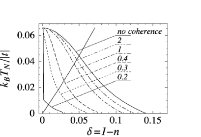
Figure 6: $T_{N}$ of the symmetric model as a function of $\delta=1-n$. From the bottom, solid, dotted, broken, dot-broken, and double-dot-broken lines show $T_{N}$ for $\gamma/|t|=0.2$, 0.3, 0.4, 1, and 2, respectively. The topmost solid line shows $T_{N}$ determined from Eq. (54) for comparison. The solid line with a positive slope shows $1/\tilde{\phi}_{\gamma}$. Antiferromagnetic states whose $T_{N}$ are much below this line are, at least, characterized as itinerant-electron ones.

         

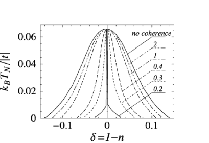
Figure 7: $T_{N}$ of the asymmetric model as a function of $\delta$. See also the caption of Fig. 6. Note that $T_{N}$ is almost symmetric between $\delta<0$ and $\delta>0$.

III.4 Almost symmetric $T_{N}$ between $\delta>0$ and $\delta<0$

When the coherent part of the Green function is not considered, $\tilde{C}_{L}=0$ and $C_{F}=0$; the instability condition (27) becomes as simple as

$$\frac{1}{\tilde{\chi}_{s}(0)}+\frac{5\Phi}{2\tilde{\chi}_{s}(0)}-\frac{1}{4}J({\bf Q})=0.$$ (54)

When the mode-mode coupling term $5\Phi/2\tilde{\chi}_{s}(0)$ is ignored and we assume $T_{K}=0$, Eq. (54) gives $T_{N}=(1/4)J({\bf Q})/k_{B}=|J|/k_{B}$, which is nothing but $T_{N}$ in the mean-field approximation for the Heisenberg model. Because Eq. (54) is what is expected for $T/T_{K}\gg 1$, Eq. (27) is valid for not only $T\ll T_{K}$ but also $T\gg T_{K}$. Then, it is, at least, qualitatively valid even for the crossover region between $T\ll T_{K}$ and $T\gg T_{K}$.

It is possible that $\gamma/|t|=O(1)$, as is examined in Appendix A. Figure 6 shows $T_{N}$ of the symmetric model as a function of $\delta=1-n$ for various $\gamma$. The region of antiferromagnetic states is wider for larger $\gamma$, mainly because $T_{K}$ is lower for larger $\gamma$. Figure 7 shows $T_{N}$ of the asymmetric model as a function of $\delta$. As long as $\gamma$ is almost symmetric with respect to $\delta$, $T_{N}$ is also almost symmetric with respect to $\delta$. The difference of the Fermi surfaces cannot give any significant asymmetry of $T_{N}$ between $\delta<0$ and $\delta>0$.

IV Application to cuprate oxides

The $t$-$J$ model with the just half filling is reduced to the Heisenberg model. The Néel temperature is as high as $T_{N}=|J|/k_{B}$ in the mean-field approximation for the Heisenberg model. It is much higher than observed $T_{N}$. This discrepancy can be explained by the reduction of $T_{N}$ by quasi-two dimensional thermal spin fluctuations or by the local mode-mode coupling term $\Lambda_{L}(0)$. When the anisotropy is as large as Eq. (53), $T_{N}$ is as low as $T_{N}\simeq 0.2|J|/k_{B}$, as is shown in Fig. 6. This explains observed $T_{N}\simeq 300$ K, when we take $|J|\simeq 0.15$ eV. However, the assumed anisotropy seems to be a little too large. We should consider the reduction of $T_{N}$ more properly than we do in this paper.

When electrons or holes are doped, Gutzwiller’s quasiparticles are formed on the chemical potential. When their life-time widths $\gamma$ or temperatures $k_{B}T$ are much larger than their bandwidth, however, quasiparticles can play no significant role. The Kondo temperature is approximately given by $k_{B}T_{K}\simeq 2|\delta t|$, with $\delta$ being the concentrations of dopants. The Néel temperature $T_{N}$ is determined by the competition between the stabilization of antiferromagnetism by the superexchange interaction $J$ and the quenching of magnetic moments by the Kondo effect with $k_{B}T_{K}$ and the local mode-mode coupling term $\Lambda_{L}(0)$. The reduction of $T_{N}$ for small $|\delta|$ is mainly due to $\Lambda_{L}(0)$, as is discussed above. On the other hand, the critical concentration $|\delta_{c}|$ below which antiferromagnetic ordering appears at $T=0$ K is mainly determined by the competition between $J$ and $k_{B}T_{K}$, because thermal spin fluctuations vanish at $T=0$ K. The critical concentration is as large as $|\delta_{c}|\simeq 0.14$ for parameters relevant for cuprates, as is shown in Figs. 6 and 7.

When both of $\gamma$ and $k_{B}T$ are small, the selfenergy-type mode-mode coupling term $\Lambda_{s}(0,{\bf Q})$ is large. Not only the linear terms in $F_{s}(i\omega_{l},{\bf q})=\chi_{s}(i\omega_{l},{\bf q})-\tilde{\chi}_{s}(0)$ but also higher order terms in $F_{s}(i\omega_{l},{\bf q})$ should be considered, for example, in a FLEX approximation. The Néel temperature $T_{N}$ is a little higher in the FLEX approximation than it is in the treatment of this paper. Unless both of $\gamma$ and $k_{B}T$ are very small, $\Lambda_{s}(0,{\bf Q})$ is much smaller than $\Lambda_{L}(0)$. In such a case, no significant correction can arise even if the treatment of $\Lambda_{s}(0,{\bf Q})$ itself is irrelevant. Relative corrections $\Delta T_{N}/T_{N}$ are large only for low $T_{N}$, for example $T_{N}/|t|\lesssim 0.005$, with $\Delta T_{N}$ an increment of $T_{N}$ in the FLEX approximation. Because $\Delta T_{N}/T_{N}$ are large only in such low $T_{N}$ regions, corrections $\Delta T_{N}$ themselves are never significant. Note that $T_{N}$ for large enough $\gamma$ or $T_{N}$ determined from Eq. (54) has no correction in the FLEX approximation.

When $\gamma$ and $k_{B}T$ are much smaller than the quasiparticle bandwidth, quasiparticles can play significant roles in not only the enhancement but also the suppression of antiferromagnetism. Antiferromagnetism is enhanced by the exchange interaction $J_{Q}(i\omega_{l},{\bf q})$ airing from the virtual exchange of pair excitations of quasiparticles, in which the nesting of the Fermi surface can play a significant role. The Fock term of the superexchange interaction renormalize quasiparticles; the bandwidth of quasiparticles is approximately given by $8|t^{*}|$, with

$$t^{*}\simeq(\pi^{2}/8)|\delta t|-\left(3\tilde{W}_{s}^{2}/2\pi^{2}\right)J,$$ (55)

in the limit of $\gamma/|t^{*}|\rightarrow+0$ and $k_{B}T/|t^{*}|\rightarrow+0$. The Kondo temperature is approximately given by $k_{B}T_{K}\simeq(1/4c_{T_{K}})|t^{*}|\simeq 1.6|t^{*}|$. The Kondo effect of quenching magnetism is stronger when $\gamma$ are smaller or quasiparticles are more itinerant. The intersite mode-mode coupling term, $\Lambda_{s}(0,{\bf Q})+\Lambda_{v}(0,{\bf Q})$, also suppresses antiferromagnetism in addition to the local mode-mode coupling term $\Lambda_{L}(0)$. Because the quenching effects overcome the enhancement effect, $T_{N}$ decrease with decreasing $\gamma$.

Physical properties are asymmetric between electron-doped $(\delta<0)$ and hole-doped $(\delta>0)$ cuprates. For example, an antiferromagnetic states appears in a narrow range of $0\leq|\delta|\lesssim 0.02$–$0.05$ in hole-doped cuprates, while it appears in a wide range of $0\leq|\delta|\lesssim 0.13$–$0.15$ in electron-doped cuprates. Tohyama and Maekawatohyama argued that the asymmetry must arises from the difference of the Fermi surfaces, and that the $t$-$t^{\prime}$-$J$ or asymmetric model should be used. They showed that the intensity of spin excitations is relatively stronger in electron doping cases than it is in hole doping cases. According to Fig. 5, the polarization function at ${\bf q}=(\pm\pi/2a,\pm\pi/2a)$ is relatively larger in electron doping cases than it is in hole doping cases. This asymmetry is consistent with that of spin excitations studied by Tohyama and Maekawa. However, the difference of the Fermi surfaces cannot explain the asymmetry of $T_{N}$, as is shown in Fig. 7.

The condensation energy at $T=0$ K of the asymmetric model is also quite asymmetric;yokoyama it is consistent with the asymmetry discussed above. On the other hand, $T_{N}$ is significantly reduced by quasi-two dimensional spin fluctuations as well as local spin fluctuations of the Kondo effect. This large reduction of $T_{N}$ arises from the renormalization of normal states; not only the Néel states but also paramagnetic states just above $T_{N}$ are largely renormalized by the spin fluctuations. It is plausible that the asymmetry of the condensation energy of paramagnetic states just above $T_{N}$ is similar to that of the Néel states at $T=0$ K. It is interesting to confirm by comparing the condensation energy of the Néel states and that of paramagnetic states just above $T_{N}$ whether $T_{N}$ is actually almost symmetric as is shown in this paper.

Electrical resistivities of electron-doped cuprates are relatively larger than those of hole-doped cuprates are.tokura A plausible explanation is that the asymmetry of $T_{N}$ arises mainly from the difference of disorder. Critical $|\delta|$’s for electron-doped cuprates below which an antiferromagnetic state appears are as large as $0.13$–$0.15$. These numbers are close to the theoretical critical value about $|\delta_{c}|=0.14$ for large $\gamma$. This implies that disorder of electron-doped cuprates must be large. In hole-doped cuprates, on the other hand, an antiferromagnetic state appear only in a narrow range of $0\leq\delta\lesssim 0.02$–0.05 although antiferromagnetic spin fluctuations are well developed in a wide range of $0\leq\delta\lesssim 0.15$. This implies that a paramagnetic state in the range of $0\leq\delta\lesssim 0.15$ is in the vicinity of an antiferromagnetic critical point. We expect that when disorder is introduced into such paramagnetic hole-doped cuprates antiferromagnetism must appear in a wide range of hole concentrations. In actual, magnetic moments appear when Zn ions are introduced.CuprateZn An almost symmetric behavior of $T_{N}$ must be restored by preparing hole-doped and electron-doped cuprates with similar degree of disorder to each other.

An antiferromagnetic state in the range of $0\leq\delta\lesssim 0.02$ of hole-doped La_2-δM_δCuO₄ (M= Sr or Ba) is characterized as a local-moment one. The so called spin-glass or Kumagai’s phaseKumagai appears in the range of $0.02\lesssim\delta\lesssim 0.05$. The $\delta$ dependence of $T_{N}$ observed for hole-doped cuprate is qualitatively different from that of theoretical $T_{N}$ shown in Figs. 6 and 7, where $\gamma$ is assumed to be constant as a function of $\delta$. Experimentally, electrical resistivities are large for under-doped cuprates. This observation implies that in general $\gamma$ is a decreasing function of $|\delta|$. For example, Fig. 8(a) shows theoretical $T_{N}$ for several cases of $\gamma(\delta)$ as a function of $\delta$, which are shown in Fig. 8(b). If we take a proper $\gamma(\delta)$, observed $T_{N}(\delta)$, including $T_{N}(\delta)$ of Kumagai’s phase, can be reproduced.

 

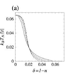
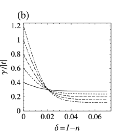
Figure 8: (a) $T_{N}$ as a function of $\delta$, and (b) $\gamma$ as a function of $\delta$. When we assume $\gamma$ shown in Fig. 8(b), we obtain $T_{N}$ shown in Fig. 8(a) by the same kind of line as that for $\gamma$.

           

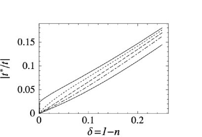
Figure 9: $t^{*}$ of the symmetric model as a function of $\delta$ for various $\gamma$ and $k_{B}T/|t|=0.02$; $\tilde{W}_{s}\simeq 1$ or $r=0.5$ is assumed instead of $\tilde{W}_{s}\simeq 2$ or $r=1$ (See text). From the top, solid, dotted, broken, and dot-broken line show $t^{*}$ for $\gamma/|t|=0.04$, 0.1, 0.2, and 0.4, respectively. For the sake of comparison, $1/\tilde{\phi}_{\gamma}$ is also shown by a bottom solid line.

           

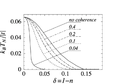
Figure 10: $T_{N}$ of the symmetric model as a function of $\delta$ for various $\gamma$; $\tilde{W}_{s}\simeq 1$ or $r=0.5$ is assumed instead of $\tilde{W}_{s}\simeq 2$ or $r=1$ (See text). From the bottom, solid, dotted, broken, and dot-broken lines show $T_{N}$ for $\gamma/|t|=0.04$, 0.1, 0.2, and 0.4, respectively. For comparison, $T_{N}$ determined from Eq. (54) is shown by a topmost solid line.

The effective three-point vertex function $\tilde{\phi}_{s}$ and the mass-renormalization factor $\tilde{\phi}_{\gamma}$ are those in SSA. They are renormalized by intersite fluctuations such as antiferromagnetic and superconducting fluctuations. We can take into account these intersite types of renormalization phenomenologically, or we can treat $\tilde{W}_{s}$ as a phenomenological parameter following the previous paper,OhkawaPseudogap where $\tilde{W}_{s}=0.7\mbox{--}1$ is used in stead of $\tilde{W}_{s}\simeq 2$ in order to explain quantitatively observed superconducting critical temperatures and $T$-linear resistivities of cuprates. Then, we replace $\tilde{W}_{s}$ by $r\tilde{W}_{s}$, with $r$ a numerical constant smaller than unity;comment-Ws Eq. (22) is replaced by

$$2t^{*}=r\frac{2t}{\tilde{\phi}_{\gamma}}-\frac{3}{4}\left(r\tilde{W}_{s}\right)^{2}J\Xi.$$ (56)

Figures 9 and 10 show $t^{*}$ and $T_{N}$, respectively, of the symmetric model as a function of $\delta$ for $r=0.5$ and various $\gamma$. The antiferromagnetic region extends with decreasing $r$, but theoretical curves for $r=0.5$ shown in Fig. 10 are qualitatively the same as those for $r=1$ shown in Fig. 6. When we take a proper $\gamma(\delta)$, we can also reproduce observed $T_{N}(\delta)$ even for $r=0.5$ or $\tilde{W}_{s}\simeq 1$.

According to Fig. 10, $\gamma/|t|\simeq 0.04$ is needed in order to reproduce Kumagai’s phase. According to Fig. 9, $|t^{*}/t|\simeq 0.05$ for $\delta=0.04$. Then, we can argue that $k_{F}l\simeq 2k_{B}T_{K}/\gamma\simeq 4|t^{*}|/\gamma$, with $k_{F}$ the Fermi wave number and $l$ the mean free path, must be 4–8 in Kumagai’s phase.ComGammaE-dep According to Fig. 4(b), the nesting of the Fermi surface is substantial at least for $\gamma/|t^{*}|\lesssim 0.3$; the nesting cannot be ignored for $\gamma/|t^{*}|\lesssim 1$. Kumagai’s phase must be a spin density wave (SDW) state in a disordered system rather than a spin glass. The divergenceKumagai of the nuclear quadrupole relaxation (NQR) rate at $T_{N}$ supports this characterization.

The so called stripe phase appears in the vicinity of $\delta=1/8$.tranquada Because superconductivity is suppressed, the pair breaking by disorder must be large; disorder may be related with a structural phase transition of first order between high-temperature tetragonal (HTT) and low-temperature orthorhombic (LTO) lattices.fujita ; fleming Then, resistivities must also be large. In actual, resistivities increase logarithmically with decreasing temperatures in LTO phase;uchida the logarithmic increase implies the Anderson localization, as is discussed below. One of possible explanations is that a SDW state enhanced by disorder is stabilized. According to Fig. 10, $\gamma/|t|\simeq 0.2$ is needed in order that an antiferromagnetic state might appear for $\delta\simeq 1/8$. On the other hand, $|t^{*}/t|\simeq 0.1$ for $\delta\simeq 1/8$. Then, we can argue that when $k_{F}l\lesssim 2$ is satisfied SDW can appear for $\delta\simeq 1/8$.ComGammaE-dep Because the strength of quenching of magnetic moments, $k_{B}T_{K}$, is an increasing function of $|\delta|$, a charge density wave (CDW) appears in such a way that the electron filling is closer to unity at sites where magnetizations are larger; the wave number of CDW is twice of that of SDW.antiferromagnetism

Because effective disorder increases with increasing magnetic fields in disordered Kondo lattices,OhkawaPositiveMR where the distribution or disorderness of $T_{K}$ is large, we argue that disordered cuprates must exhibit large positive magnetoresistance and antiferromagnetic ordering must be induced by magnetic fields. It is interesting to examine whether the stripe state exhibits large positive magnetoresistance and the critical temperature of the stripe state is enhanced by magnetic fields.

For the sake of simplicity, we assume that ordering wave numbers Q are commensurate. However, Q are incommensurate for large $|\delta|$, as is shown in Fig. 5. When incommensurate Q are considered, $T_{N}$ become a little higher than they are in this paper. According to Ref. antiferromagnetism, , when Q are incommensurate and a tetragonal lattice distortion is small enough, a double-Q SDW with magnetizations of different Q being orthogonal to each other can be stabilized on each CuO₂ plane. It is interesting to look for such non-colinear magnetic structure.

The Fock term of the superexchange interaction between nearest neighbors renormalizes only nearest-neighbor $t^{*}$, but it does not renormalize next-nearest-neighbor $t_{2}^{*}$. The ratio of $t_{2}^{*}/t^{*}$, which is assumed to be constant in this paper, must depend on various parameters such as $\gamma$, $T$, $\delta=1-n$, and so on. For example, Fig. 9 shows $t^{*}$ as a function of $\delta$ for various $\gamma$, $k_{B}T/|t|=0.02$, and $\tilde{W}_{s}\simeq 1$ $(r=0.5)$. In case of $\tilde{W}_{s}=0.7\mbox{--}1$, the magnitude of the renormalization of $t^{*}$ due to the Fock term is about a eighth or a fourth of those shown in Figs. 1 and 2, where $\tilde{W}_{s}\simeq 2$ is assumed. Although the renormalization is expected to be rather small in actual cuprates, it is interesting to examine the dependence of the shape of the Fermi surface or line on such parameters, in particular, on $\gamma$. The shape of the Fermi surface must be more similar to what the symmetric model predicts in better samples with smaller $\gamma$ than it is in worse samples with large $\gamma$. This argument also leads to a prediction that because of the Fock term, if the broadening due to $\gamma$ is corrected, the bandwidth of quasiparticles must be larger in better samples than it is in worse samples.

The bandwidth of Gutzwiller’s quasiparticles is of the order of $|J|$ at $T=0$ K for the Hubbard model with no disorder and the just half filling, even when $\tilde{\phi}_{\gamma}\rightarrow+\infty$.exchByOhkawa Because $J=-4t^{2}/U$ for large enough $U/|t|$, the bandwidth vanishes only in the limit of $U/|t|\rightarrow+\infty$. We speculate that, if the Hilbert space is restricted within paramagnetic states, the disappearance of Gutzwiller’s band or the metal-insulator transition considered by Brinkman and RiceBrinkman must occur at $U\rightarrow+\infty$. When the critical $U_{c}$ is infinitely large, no hidden order parameter is required in this transition of second order. When small disorder is introduced or temperatures are slightly raised, the transition at $U\rightarrow+\infty$ must turn out to a crossover around a finite $U$; the $U$ must be very close to what Brinkman and Rice’s theory predicts, unless disorder and $k_{B}T$ are extremely small.

In actual metal-insulator transitions, which are of first order, the symmetry of a lattice changes or the lattice parameter discontinuously changes. Within a single-band model with no electron-phonon interaction, it is difficult, presumably impossible, to reproduce first-order metal-insulator transitions. The electron-phonon interaction as well as orbital degeneracy should be included in order to explain actual metal-insulator transitions of first order.

One of the most serious assumptions in this paper is the homogeneous life-time width of quasiparticles. This assumption is irrelevant when the concentration of dopants is small. For example, introduce a single metal ion such as Sr in a purely periodic La₂CuO₄. A hole must be bound around the metal ion. When the concentration of metal ions is small enough, each hole must be similarly bound around each metal ion or it is in one of the Anderson localized states. The Anderson localization may play a role at low temperatures; we expect the logarithmic dependence of resistivities on temperatures in two dimensions as well as negative magnetoresistance. In actual, logarithmic divergent resistivities with decreasing temperatures are observed.ono However, observed magnetoresistance is positive rather than negative.miura Because positive magnetoresistance is expected in disordered Kondo lattices,OhkawaPositiveMR as is discussed above, one of the possible explanations is that the positive magnetoresistance due to the disorderness of $T_{K}$ cancels or overcomes the negative magnetoresistance due to the Anderson localization. The Anderson localization in disordered Kondo lattices should be seriously considered to clarify electronic properties of cuprates with rather small concentrations of dopants or under-doped cuprates.

V Conclusion

Effects of life-time widths $\gamma$ of quasiparticles on the Néel temperature $T_{N}$ of the $t$-$J$ model with $J/|t|=-0.3$ on a quasi-two dimensional lattice are studied within a theoretical framework of Kondo lattices. The Kondo temperature $T_{K}$, which is a measure of the strength of the quenching of magnetism by local quantum spin fluctuations, is renormalized by the superexchange interaction $J$, so that $T_{K}\simeq\left(-c_{J}J+2|\delta t|\right)/k_{B}$, with $c_{J}$ a positive numerical constant, $\delta$ the concentration of dopants, holes $(\delta>0)$ and electrons $(\delta<0)$, and $k_{B}$ the Boltzmann constant. The renormalization term $-c_{J}J$ depends on $\gamma$. The bandwidth $W^{*}$ of quasiparticles is about $4k_{B}T_{K}$.

When $\gamma\gtrsim W^{*}$, it follows that $c_{J}\ll 1$; the quenching of magnetism by the Kondo effect is weak. Quasi-two dimensional thermal spin fluctuations make $T_{N}$ substantially reduced; $T_{N}\simeq 0.2|J|/k_{B}$ for $\delta=0$, when an exchange interaction $J_{z}$ between nearest-neighbor planes is as small as $|J_{z}/J|\simeq 10^{-10}$. This explains observed $T_{N}\simeq 300$ K for $\delta=0$ in cuprates, if we take $|J|\simeq 0.15$ eV. Because thermal spin fluctuations vanish at $T=0$ K, however, an antiferromagnetic state is stabilized in a wide range of $\delta$ such as $0\leq|\delta|\lesssim 0.14$ for $J/|t|=-0.3$. When $T_{N}\gg T_{K}$, an antiferromagnetic state is characterized as a local-moment one. When $T_{N}\ll T_{K}$, it is characterized as an itinerant-electron one rather than a spin glass.

When $\gamma\ll W^{*}$, it follows that $c_{J}=O(1)$; the quenching by the Kondo effect is strong. When the nesting of the Fermi surface is substantial, the exchange interaction arising from the virtual exchange of pair excitations of quasiparticles is also responsible for antiferromagnetic ordering in addition to the superexchange interaction. However, an antiferromagnetic state can only be stabilized for small $|\delta|$ because not only quasi-two dimensional thermal spin fluctuations but also the Kondo effect with high $T_{K}$ make $T_{N}$ substantially reduced or they destroy antiferromagnetic ordering; the critical $|\delta|$ below which antiferromagnetic ordering appears is smaller for smaller $\gamma$. An antiferromagnetic state in this case is characterized as an itinerant-electron one.

The life-time width of quasiparticles arising from disorder must be a crucial parameter for cuprates. The difference of disorder must be mainly responsible for the asymmetry of $T_{N}$ between electron-doped and hole-doped cuprates; disorder must be relatively larger in electron-doped cuprates than it is in hole-doped cuprates. It is interesting to examine if an almost symmetric behavior of $T_{N}$ is restored by preparing hole-doped and electron-doped cuprates with similar degree of disorder to each other. Because effective disorder can be enhanced by magnetic fields, it is also interesting to look for magnetic-field induced antiferromagnetic ordering in cuprates that exhibit large magnetoresistance.

Appendix A Scattering potential in disordered Kondo lattices

In disordered Kondo lattices, the mapped Anderson models are different from site to site. When the perturbative expansion for a single-impurity systemYamada is extended to include the site dependence, the selfenergy for the $j$th site is expanded in such a way that

$$\tilde{\Sigma}_{j\sigma}(\varepsilon\!+\!i0) = \tilde{\Sigma}_{j\sigma}(0)+\left(1-\tilde{\phi}_{j\gamma}\right)\varepsilon$$ (57)

$$-i\frac{\tilde{\phi}_{js}\!-\!\tilde{\phi}_{j\gamma}}{2\Delta_{j}(0)}\left[\varepsilon^{2}\!+\!(\pi k_{B}T)^{2}\right]\!+\cdots,\qquad$$

with $\Delta_{j}(\varepsilon)$ the hybridization energy of the $j$th Anderson model. When its energy dependence is ignored, it follows according to Shibashiba that

$$E_{dj}+\tilde{\Sigma}_{j\sigma}(+i0)=\Delta_{j}(0)\tan\left[\pi\left(\mbox{$\frac{1}{2}$}-n_{j\sigma}\right)\right],$$ (58)

with $n_{j\sigma}$ the number of electrons with spin $\sigma$ at the $j$th site. Here, $E_{dj}$ is the localized-electron level of the $j$th mapped Anderson model; it is equal to the band center of the $t$-$J$ model, so that $E_{dj}=0$. It follows from Eqs. (24) and (25) that $\tilde{\phi}_{j\gamma}\simeq(\pi^{2}/8)/|1-n_{j}|$ and $\tilde{\phi}_{js}\simeq(\pi^{2}/4)/|1-n_{j}|$ for almost half filling $n_{j}\equiv n_{j\uparrow}+n_{j\downarrow}\simeq 1$. We assume non-magnetic impurities so that $n_{j\uparrow}=n_{j\downarrow}$.

The average number of $n_{j}$ and its mean-square deviation are given by

$$\hskip 10.0ptn=\int\!\!dxN_{imp}(x)x,$$ (59)

$$\hskip-10.0pt\Delta n^{2}=\int\!\!dxN_{imp}(x)\left(x-n\right)^{2},$$ (60)

with $N_{imp}(n_{j})$ the distribution of $n_{j}$. We assume that there is no correlation among disorder at different sites in our ensemble of disordered systems.

We can consider the site-dependent part of the single-site selfenergy as a static scattering potential. It is approximately given by

$$V_{j\sigma}(\varepsilon)=-\left(\frac{\pi\Delta}{2}+\frac{8}{\pi^{2}}\tilde{\phi}_{\gamma}^{2}\varepsilon\right)(n_{j}\!-\!n)\frac{1\!-\!n}{|1\!-\!n|}+\cdots.$$ (61)

Disorder of $n_{j}$ arises from that of $\Delta_{j}(\varepsilon)$; in Eq. (61), their site and energy dependences are ignored and they are simply dented by $\Delta$. When we treat this energy-dependent scattering potential in the second-order SSA or the Born approximation, the coherent part of the ensemble averaged Green function is given by

$$\left<g_{\sigma}^{(0)}(\varepsilon+i0,{\bf k})\right>_{dis} = \frac{1}{\tilde{\phi}_{\gamma}}\frac{1}{\displaystyle\varepsilon+i0+\mu^{*}-\xi({\bf k})-(1/\tilde{\phi}_{\gamma})\Sigma_{\sigma}^{dis}(\varepsilon+i0)},$$ (62)

with

$$\frac{1}{\tilde{\phi}_{\gamma}}\Sigma_{\sigma}^{dis}(\varepsilon\!+\!i0)=-i\frac{\pi}{\tilde{\phi}_{\gamma}^{2}}\left[\frac{\pi\Delta}{2}\!+\!\frac{8}{\pi^{2}}\tilde{\phi}_{\gamma}^{2}\varepsilon\right]^{2}\!\!\Delta n^{2}\rho_{\gamma}(\varepsilon),$$ (63)

for $|\varepsilon|\lesssim k_{B}T_{K}$. Here, $\left<\cdots\right>_{dis}$ stands for an ensemble average over disordered systems.

The bandwidth of quasiparticles is about $4k_{B}T_{K}$, so that typical life-time width is as large as

$$\frac{1}{\tilde{\phi}_{\gamma}}\mbox{Im}\Sigma_{\sigma}^{dis}(\pm k_{B}T_{K}+i0)\simeq-i(64/\pi^{3})\tilde{\phi}_{\gamma}\Delta n^{2}|t|.$$ (64)

The energy-independent term can be ignored because $\tilde{\phi}_{\gamma}\gg 1$ for almost half fillings. It is quite likely that $\tilde{\phi}_{\gamma}\Delta n^{2}=O(1)$ and $\gamma/|t|=O(1)$ for almost half fillings.

It is straightforward to extend the above argument to a system in the presence of magnetic fieldsOhkawaPositiveMR and a system with magnetic impurities. In such cases, $n_{i\uparrow}-n_{i\downarrow}$ can be different from site to site; $\mbox{Im}\Sigma_{\sigma}^{dis}(\varepsilon+i0)/\tilde{\phi}_{\gamma}$ can be large even on the chemical potential $(\varepsilon=0)$.

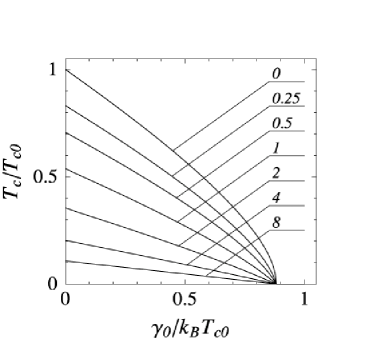
Figure 11: Superconducting $T_{c}$ as a function of static pair breaking $\gamma_{0}$ for $\nu=0$, 0.25, 0.5, 1, 2, 4 and 8; $\gamma=\gamma_{0}+\nu k_{B}T$ is assumed as the total pair breaking. The result for $\nu=0$ is nothing but that by the AG theory.abrikoso-gorkov

Appendix B Deviation from the Abrikosov-Gorkov theory

The reduction of superconducting $T_{c}$ by pair breaking is approximately given by the Abrikosov-Gorkov (AG) theory:abrikoso-gorkov

$$-\ln\left(\frac{T_{c}}{T_{c0}}\right)=\psi\left(\frac{\gamma}{2\pi k_{B}T_{c}}+\frac{1}{2}\right)-\psi\left(\frac{1}{2}\right),$$ (65)

with $T_{c0}$ critical temperatures in the absence of any pair breaking or for vanishing life-time widths ($\gamma=0$). We assume that life-time widths are given by $\gamma=\gamma_{0}+\nu k_{B}T$, where $\gamma_{0}$ arises from static scatterings by disorder and $\nu k_{B}T$ arises from inelastic scatterings by thermal spin and superconducting fluctuations; both experimentally and theoretically, the contribution from thermal fluctuations to $\gamma$ is almost linear in $T$ except at very low temperatures. Figure 11 shows $T_{c}$ as a function of $\gamma_{0}$ for various $\nu$. It is interesting that the reduction of $T_{c}$ is almost linear in $\gamma_{0}$ for large enough $\nu$ such as $\nu\gtrsim 2$.

According to the previous paper published in 1987,Ohkawa87SC-2 the ratio of $\epsilon_{G}(0)/k_{B}T_{c}$, with $\epsilon_{G}(0)$ superconducting gaps at $T=0$ K, is as large as $4.35$ for $d\gamma$ wave. However, observed ratios are larger than that, for example, $\epsilon_{G}(0)/k_{B}T_{c}\simeq 8$ for optimal-doped cuprates and $\epsilon_{G}(0)/k_{B}T_{c}\gg 8$ for under-doped cuprates. This discrepancy can be explained in terms of the temperature dependent pair breaking, because it reduces $T_{c}$ but it does not reduce $\epsilon_{G}(0)$.OhkawaPseudogap Considering observed ratios of $\epsilon_{G}(0)/k_{B}T_{c}$ and Fig. 11, we argue that $\nu=1\mbox{--}2$ for optimal-doped cuprates and $\nu\gg 2$ for under-doped cuprates. When $\nu\gtrsim 2$, the reduction of $T_{c}$ is almost linear in $\gamma_{0}$. According to a recent observation,alloul in actual, the reduction of $T_{c}$ is almost linear in the dose of electron irradiation.

References

- (1) J.G. Bednortz and K.A. Müller, Z. Phys. B 64, 189 (1986)
- (2) See for example, H. Takagi, Y. Tokura, and S. Uchida, Physica C 162-164, 1001 (1989).
- (3) J. Kanamori, Prog. Theor, Phys. 30, 275 (1963).
- (4) J. Hubbard, Proc. Roy. Soc. London Ser. A 276, 238 (1963); A 281, 401 (1964).
- (5) M.C. Gutzwiller, Phys. Rev. Lett. 10, 159 (1963); Phys. Rev. A 134, 293 (1963); A 137, 1726 (1965).
- (6) J.M. Luttinger and J.C. Ward, Phys. Rev. 118, 1417 (1960).
- (7) J.M. Luttinger, Phys. Rev. 119, 1153 (1960).
- (8) F.J. Ohkawa, J. Phys. Soc. Jpn. 58, 4156 (1989).
- (9) W.F. Brinkman and T.M. Rice, Phys. Rev. B 2, 4302 (1970).
- (10) Such an SSA may include the renormalization of single-site terms by intersite effects, as is shown in Sec. II.1 of this paper.
- (11) F.J. Ohkawa, Phys. Rev. B 44, 6812 (1991); J. Phys. Soc. Jpn. 60, 3218 (1991); 61, 1615 (1992).
- (12) K. Yosida, Phys. Rev. 147, 223 (1966),
- (13) P. W. Anderson, J. Phys. C 3, 2436 (1970).
- (14) K. G. Wilson, Rev. Mod. Phys. 47, 773 (1975).
- (15) P. Nozières, J. Low. Temp. Phys. 17, 31 (1974).
- (16) K. Yamada, Prog. Theor. Phys. 53, 970 (1975); 54, 316 (1975).
- (17) K. Yosida and K. Yamada, Prog. Theor. Phys. 53, 1286 (1970).
- (18) F.J. Ohkawa, J. Phys. Soc. Jpn. 67, 535 (1998).
- (19) E. Miyai and F.J. Ohkawa, Phys. Rev. B 61, 1357 (2000).
- (20) H. Satoh and F.J. Ohkawa, Phys. Rev. B 57, 5891 (1998); B 63, 184401 (2001).
- (21) F.J. Ohkawa, J. Phys. Soc. Jpn. 67, 535 (1998); Phys. Rev. B 66, 014408 (2002).
- (22) F.J. Ohkawa, Phys. Rev. B 65, 174424 (2002).
- (23) F.J. Ohkawa, Phys. Rev. B 59, 8930 (1999).
- (24) F.J. Ohkawa, Physica B 281-282, 859 (2000).
- (25) F.J. Ohkawa, J. Phys. Soc. Jpn. 69, Suppl. A 13 (2000).
- (26) F.J. Ohkawa, Phys. Rev. B 69, 104502 (2004).
- (27) F.J. Ohkawa, cond-mat/0405703 (unpublished). Because the electron-phonon interaction proposed in this paper is enhanced by spin and superconducting fluctuations, its effective strength depends on and . Although it renormalizes the quasiparticle dispersion, it can play no significant role in the formation of -wave Cooper pairs in cuprate oxide superconductors.
- (28) F.J. Ohkawa, Jpn. J. Appl. Phys. 26, L652 (1987).
- (29) F.J. Ohkawa, J. Phys. Soc. Jpn. 56, 2267 (1987).
- (30) F.J. Ohkawa, J. Phys. Soc. Jpn. 61, 631 (1992); 61, 952 (1992); 61, 1157 (1992).
- (31) A.A. Abrikosov and L.P. Gorkov, Sov. Phys. JETP 12, 1243 (1960).
- (32) Considering the virtual exchange of pair excitations of electrons between the lower and upper Hubbard bands, we can derive the superexchange interaction by the field-theoretical method: It was derived in F.J. Ohkawa, J. Phys. Soc. Jpn. 61, 1615 (1992) for the auxiliary-particle or slave-boson Hubbard model, F.J. Ohkawa, J. Phys. Soc. Jpn. 63, 602 (1994) for the Hubbard model, Ref. ferromagnetism, for the multi-band Hubbard model, Ref. OhkawaSC1, for the - model, and F.J. Ohkawa, J. Phys. Soc. Jpn. 67, 525 (1998) for the periodic Anderson model. Because its energy dependence can be ignored for low energies such as or , we obtain similar renormalization of by the superexchange interaction even in the Hubbard, -, and periodic Anderson models.
- (33) Because of this simplification, we can carry out analytically summations over Matsubara’s frequencies in many equations of this paper.
- (34) J.C. Ward, Phys. Rev. 68, 182 (1950).
- (35) Two mechanisms of the formation of Cooper pairs by the superexchange interaction and the spin-fluctuation mediated interaction are essentially the same as each other. When low-energy spin fluctuations, whose energies are much smaller than , are only considered, however, they are physically different from each other.
- (36) A. Kawabata, J. Phys. F 4, 1447 (1974).
- (37) F.J. Ohkawa, Phys. Rev. B 57, 412 (1998).
- (38) T. Tohyama and S. Maekawa, Phys. Rev. B 49, 3596 (1994).
- (39) H. Yokoyama, T. Tanaka, M. Ogata, and H. Tsuchiura, cond-mat/0308264 (unpublished).
- (40) A. Sawa, M. Kawasaki, H. Takagi, and Y. Tokura, Phys. Rev. B 66, 014531 (2002).
- (41) H. Alloul, P. Mendels, H. Casalta, J.F. Marucco, and J. Arabski, Phys. Rev. Lett. 67, 3140 (1991).
- (42) K. Kumagai, I. Watanabe, H. Aoki, Y. Nakamura, T. Kimura, Y. Nakamichi, and H. Nakajima, Physica 148B 480, (1987).
- (43) In Eqs. (29) and (30), we should use a multiplication factor slightly different from because appearing there is a purely single-site property. In the first term of Eq. (56), we should also use another one slightly different from because no appears there. However, we assume the same in every equation for the sake of simplicity.
- (44) When the energy dependence of is taken into account can be larger than the estimation of this paper is.
- (45) J.M. Tranquada, B.H. Stenlieb, J.D. Axe, and S. Uchida, Nature (London) 375, 561 (1995).
- (46) T. Fujita, Y. Aoki, Y. Maeno, J. Sakurai, H. Fukuba, and H. Fujii, Jpn. J. Appl. Phys. 26, L368 (1987).
- (47) R.M. Fleming, B. Batlogg, R.J. Cava, and E.A. Rietman, Phys. Rev. B 35, 7191 (1987).
- (48) Y. Nakamura and S. Uchida, Phys. Rev. B 46, 5841 (1992).
- (49) F.J. Ohkawa, Phys. Rev. Lett. 64, 2300 (1990).
- (50) S. Ono, Y. Ando, T. Murayama, F.F. Balakirev, J.B. Betts, and G.S. Boebinger, Phys. Rev. Lett. 85, 638 (2000).
- (51) N. Miura, H. Nakagawa, T. Sekitani, M. Naito, H. Sato, and Y. Enomoto, Physica B 319, 310 (2002).
- (52) H. Shiba, Prog. Theor. Phys. 54, 967 (1975).
- (53) F. Rullier-Albenque, H. Alloul, and R. Tourbot, Phys. Rev. Lett 91, 047001 (2003).