Islands in the Stream:
Electromigration-Driven Shape Evolution
with Crystal Anisotropy

Abstract.

We consider the shape evolution of two-dimensional islands on a crystal surface in the regime where mass transport is exclusively along the island edge. A directed mass current due to surface electromigration causes the island to migrate in the direction of the force. Stationary shapes in the presence of an anisotropic edge mobility can be computed analytically when the capillary effects of the line tension of the island edge are neglected, and conditions for the existence of non-singular stationary shapes can be formulated. In particular, we analyse the dependence of the direction of island migration on the relative orientation of the electric field to the crystal anisotropy, and we show that no stationary shapes exist when the number of symmetry axes is odd. The full problem including line tension is solved by time-dependent numerical integration of the sharp-interface model. In addition to stationary shapes and shape instability leading to island breakup, we also find a regime where the shape displays periodic oscillations.

1. Introduction

The interest of researchers in the phenomenon of electromigration has in the past mainly been guided by the technological implications of this effect, namely the degeneration of integrated circuits [1, 2, 3]. A large body of experimental work has been devoted to the study of electromigration-induced failure of metallic conductor lines under accelerated testing conditions [2, 4, 5, 6]. At least for simple geometries (e.g., a single void in a single crystal grain), such experiments have been successfully modeled using a macroscopic continuum theory of shape evolution [5, 7] (see Sect.2). On the other hand, theorists have conducted a lively (and still ongoing) debate on the microscopic driving force of electromigration [8, 9].

What appears to be largely missing in the field is experimental and theoretical work on the mesocopic level, addressing the evolution of simple atomic-scale structures such as individual steps and single-layer islands. This could help to bridge the gap between the elementary moves of single atoms and the failure behavior of polycrystalline conductor lines with a complex internal geometry. In the present paper we address the electromigration-induced shape evolution of single, atomic-height islands on a crystal surface. We work in a continuum setting first introduced, in this context, by Pierre-Louis and Einstein [10]. Among the different kinetic regimes considered in their work, we focus here on the particularly simple case where mass transport is exclusively along the island edge, so that the area of the island is strictly conserved and the evolution law for the island boundary is local. Our new contribution consists in including crystal anisotropy, which is clearly necessary to make contact with island electromigration on real crystal surfaces (such as silicon [11, 12]) and in lattice Monte Carlo simulations [10, 13, 14].

The continuum model is introduced in the next section, and previous work on the problem is described. In Section 3 we show how stationary shapes can be explicitly computed when the smoothening effects of the edge free energy is neglected, and numerical results for the full, time-dependent problem are presented in Section 4.

2. Continuum Model of Shape Evolution

The physical system consists of an island of monoatomic height on an otherwise flat crystal surface in interaction with the flow of the electrons. The island should be large enough to allow for a coarse grained description where the individual particles of the assembly are blurred into a continuous entity. To put this into a mathematical setting we represent the spatial conformation by a closed curve in the $xy$-plane parametrised by the arclength $s$. All geometrical and physical quantities can now be expressed as functions of $s$. We describe the local orientation of the island edge by the angle $\theta$ between the normal and the $y$-axis (counted positive in the clockwise direction). The derivative of $\theta$ with respect to $s$ is then the local curvature $\kappa$. The force $F$ acting on an atom at the island edge is composed of two contributions:

$$F=-\frac{\partial}{\partial s}(\tilde{\gamma}\kappa)+F_{el}.$$ (2.1)

Here $\tilde{\gamma}\kappa$ is the chemical potential of the island edge, with $\tilde{\gamma}$ denoting the edge stiffness, which is related to the step free energy $\gamma(\theta)$ by $\tilde{\gamma}=\gamma+d^{2}\gamma/d\theta^{2}$ [15]. The gradient of the chemical potential on the right hand side of (2.1) accounts for the effect of capillarity which tends to minimize the free energy by driving material away from regions of high curvature. The second term is the force that actually causes electromigration. It is conventionally written in the form $F_{el}=eZ^{\ast}E_{t}$, where $e$ is the elementary charge, $E_{t}$ is the component of the local electric field which acts tangentially to the step edge, and $Z^{\ast}$ is the effective valence of the step atom. On this level of modeling, all microscopic aspects of electromigration are lumped into the quantity $Z^{\ast}$. To give an example, the effective valence for a copper atom moving along a close-packed step on the Cu(100) surface has been calculated to be $Z^{\ast}\approx-31$ [14]. The form of the tangential electric field to be used in this work will be specified later.

The motion of the atoms along the edge can now be described by a mass current $j$ that is proportional to the acting force, with the factor of proportionality defining the orientation-dependent step edge mobility $\sigma(\theta)$,

$$j=\sigma(\theta)F.$$ (2.2)

If we assume that atoms can neither detach from the island nor attach to it, the equation of shape evolution is simply the continuity equation that relates the divergence of the mass current to the normal velocity $v_{n}$ of the island edge, as

$$v_{n}=-\frac{\partial}{\partial s}j=\frac{\partial}{\partial s}\sigma(\theta)[\frac{\partial}{\partial s}(\tilde{\gamma}\kappa)-eZ^{\ast}E_{t}].$$ (2.3)

By dimensional analysis, the comparison of the two terms inside the square brackets on the right hand side of (2.3) defines the characteristic length scale [10, 16, 17]

$$l_{E}=\sqrt{\frac{\tilde{\gamma}}{|eZ^{\ast}E_{0}|}},$$ (2.4)

where $E_{0}$ is a typical value of the electric field strength. For islands small compared to $l_{E}$ the capillary forces dominate the evolution, while for islands large compared to $l_{E}$ the evolution is dominated by the electromigration force. Thus $l_{E}$ sets the length scale on which electromigration-induced shape instabilities can be expected.

As formulated so far, the model is identical to the one that has been used extensively to model the evolution of quasi-two-dimensional (cylindrical) voids in current-carrying metallic thin films [5, 7, 18, 19, 20, 21, 22, 23, 24, 16, 25, 26, 27, 28]. In that context it is essential to take into account the effect of current crowding, which refers to the fact that current lines cannot pass through the insulating void, and hence the electric field is enhanced in the remaining parts of the conductor. As it is necessary to monitor the changes in the electric current configuration that occur in response to the shape changes of the void, the dynamical evolution becomes manifestly nonlocal. In the physical situation of interest in the present paper, this complication does not arise, since a single-layer island is not expected to significantly modify the electric current configuration in the underlying substrate film. We may therefore assume a constant electric field of strength $E_{0}$ directed at an angle $\phi$ with respect to the $x$-axis, and set $E_{t}=E_{0}\cos(\theta+\phi)$ in (2.3).

A model that interpolates between the case of a completely insulating void and the case of a constant electric field considered here is obtained by assigning a conductivity $\Sigma^{\prime}$ to the void which differs from the conductivity $\Sigma$ of the bulk material [18, 19]. The two limiting cases then correspond to $\Sigma^{\prime}/\Sigma=0$ and $\Sigma^{\prime}/\Sigma=1$. The local model with $\Sigma^{\prime}/\Sigma=1$ has also been used to describe the electromigration-driven evolution of dislocation loops [29, 30].

Our primary aim in this paper will be to determine the stationary shapes of the drifting island. The condition for an island to move at constant velocity $V$ along the $x$-axis without changing its shape is

$$v_{n}=V\sin(\theta).$$ (2.5)

It has been shown long ago that in the absence of anisotropy ($\tilde{\gamma}$ and $\sigma$ independent of $\theta$) a circle is a stationary solution of (2.3), for general conductivity ratio $\Sigma^{\prime}/\Sigma$ [18]. In the following we try to find corresponding results for the anisotropic case.

3. Analysis in the Absence of Capillarity

Combining the equation of motion (2.3) and the stationarity condition (2.5) gives

$$\frac{\partial}{\partial s}\sigma(\theta)[\frac{\partial}{\partial s}(\tilde{\gamma}\kappa)-F_{0}\cos(\theta+\phi)]=V\sin(\theta)$$ (3.1)

with $F_{0}=eZ^{\ast}E_{0}$. This is a nonlinear ordinary differential equation of fourth order for the shape, or alternatively of second order, when viewed as an equation for the curvature as a function of $\theta$ (using $\frac{\partial}{\partial s}=\kappa\frac{\partial}{\partial\theta}$). In this section the capillarity term proportional to the stiffness $\tilde{\gamma}$ will be neglected. While it is true that the effects of capillarity become small for large islands (island radius $\gg l_{E}$), it can hardly be justified to drop this term altogether, because it contains the highest order derivative in the equation. In fact islands that are large compared to $l_{E}$ break apart, rather than reaching a steadily drifting shape [10] (see Sect.4).

Nevertheless the analysis of the capillarity-free case $\tilde{\gamma}=0$ is rather instructive. It is accessible to an analytical treatment, because the unknown curvature enters (3.1) only through the derivative $\frac{\partial}{\partial s}$ which can be eliminated by the following substitution: From the two geometrical relations

$$(ds)^{2}=(dx)^{2}+(dy)^{2}\Leftrightarrow\left(\frac{\partial x}{\partial s}\right)^{2}+\left(\frac{\partial y}{\partial s}\right)^{2}=1$$ (3.2)

and

$$\tan(\theta)=-\frac{dy}{dx}=-\frac{\;\frac{\partial y}{\partial s}\;}{\frac{\partial x}{\partial s}}$$ (3.3)

we conclude that $\frac{\partial y}{\partial s}=-\sin(\theta)$. Replacing $\sin(\theta)$ in (3.1) using this relation we find that the derivative of $Vy-j$ is zero and therefore [29] $Vy=j+const$. The constant of integration can be set to zero, since it generates only a vertical displacement. Hence the $y$-coordinate of the island shape as a function of $\theta$ is

$$y(\theta)=\frac{F_{0}}{V}\sigma(\theta)\cos(\theta+\phi)$$ (3.4)

and using $\frac{dy}{dx}=-\tan(\theta)$ once more, we obtain

$$x(\theta)=-\int_{0}^{\theta}\cot(\theta^{\prime})\frac{\partial y}{\partial\theta^{\prime}}\,d\theta^{\prime}.$$ (3.5)

In order to derive stationary island shapes from (3.4) and (3.5) one has to specify the mobility $\sigma(\theta)$. To mimic the anisotropy of a crystal surface with a certain discrete rotational symmetry, we choose [16]

$$\sigma(\theta)=\frac{\sigma_{0}[1+S\cos^{2}(D(\theta+\alpha))]}{1+S\cos^{2}(D\alpha)}$$ (3.6)

where $\alpha$ is the angle between the symmetry axes and the coordinate system, $2D$ is the number of symmetry axes, and $S\geq 0$ is a measure for the strength of the anisotropy; see Fig.6 for an illustration of (3.6). The denominator ensures that the mobility at $\theta=0$ is $\sigma_{0}$.

3.1. Existence of stationary shapes

When calculating the shape by means of (3.4) and (3.5) with a given choice of $D,S,\alpha$ and $\phi$, one encounters two types of irregularities: (i) The curve is generally not closed, and (ii) it can contain self-intersections. To get a closed shape one has to demand that $x$ and $y$ are $2\pi$-periodic functions of $\theta$. Because $y(\theta)$ is always $2\pi$-periodic it suffices to have

$$\int_{0}^{2\pi}dx(\theta)=\int_{0}^{2\pi}d\theta\;\cot(\theta)[\frac{d\sigma}{d\theta}\cos(\theta+\phi)-\sigma\sin(\theta+\phi)]=0.$$ (3.7)

For integer values of $D$ (even rotational symmetry) the mobility is $\pi$-periodic and hence the integrand in (3.7) is odd under shifts $\theta\to\theta+\pi$. As a consequence (3.7) is always fulfilled. For half-integer $D$ (odd rotational symmetry) the evaluation of the integral in (3.7) yields $2D\cos(\phi)\cos(2D\alpha)-\sin(\phi)\sin(2D\alpha)$ times a nonzero factor, so that (3.7) requires that

$$\tan(2D\alpha)\tan(\phi)=2D.$$ (3.8)

Figure 1. Formation of self-intersections in the capillarity-free case. The figure shows stationary shapes for $D=3$ and $\alpha-\phi=0$, where the critical anisotropy strength is $S_{c}\approx 0.35.$

The generation of self-intersections is illustrated in Fig.1. Because the self-intersections are always accompanied by singularities (sign changes) of the curvature, they can be avoided by requiring that

$$\frac{1}{\kappa}=-\frac{1}{\sin(\theta)}\frac{\partial y}{\partial\theta}>0$$ (3.9)

everywhere. Thus the smoothness condition is related to the existence of extrema of $y(\theta)$. If $\frac{\partial y}{\partial\theta}$ is nonzero at $0$ or $\pi$, the integral in (3.5) diverges because it contains the singularity of the cotangent function; the shape is then not bounded. If $\frac{\partial y}{\partial\theta}$ is zero somewhere else (3.9) is violated. If $D$ is half-integer, the condition $\frac{\partial y}{\partial\theta}(0)=\frac{\partial y}{\partial\theta}(\pi)=0$ requires $\alpha=\phi=0$, which violates (3.8). In other words: For half-integer values of $D$ the shape is either not closed or not bounded. While this result has been derived using the specific functional form (3.6) for the mobility, we expect it to be true in general that in the capillarity-free case, no stationary shapes exist when the number of symmetry axes is odd.

In the following we may therefore restrict ourselves to anisotropies of even symmetry. In this case $\frac{\partial y}{\partial\theta}(0)=\frac{\partial y}{\partial\theta}(\pi)$ because of the $\pi$-periodicity of $y$ and we end up with two conditions,

$$\frac{\partial y}{\partial\theta}(0)=0 \Leftrightarrow \frac{SD\sin(2D\alpha)}{1+S\cos^{2}(D\alpha)}=-\tan(\phi)$$ (3.10)

$$\frac{\partial y}{\partial\theta}(\theta)\neq 0 \Leftrightarrow \frac{SD\sin(2D(\theta+\alpha))}{1+S\cos^{2}(D(\theta+\alpha))}\neq-\tan(\theta+\phi)\;\;\mbox{if}\;\;\theta\neq 0,\pi.$$ (3.11)

For a given value of the angle $\alpha-\phi$ between the symmetry axes and the field, (3.10) determines the direction of motion of the island, and the inequality (3.11) determines the values of $S$ for which a smooth shape exists. For $S=0$ there is always such a shape for every choice of $\alpha-\phi$, namely the circle which moves in the direction of the applied field. Increasing the anisotropy strength $S$ the circle elongates along the field direction and finally at some critical value $S_{c}$ sharp corners develop as precursors of self-intersections (see Fig.1). For $S>S_{c}$ no stationary shapes exist. Figure 2 shows the array of possible shapes for the case of sixfold symmetry ($D=3$). Note that in the absence of capillarity the characteristic scale (2.4) disappears from the problem, and hence the shapes are independent of island size (the island size determines however the migration speed, see Sect. 3.3).

Figure 2. Stationary island shapes without capillarity, for sixfold crystal anisotropy and different values of the angle $\alpha-\phi$ between the symmetry axis of the anisotropy and the field, and the anisotropy strength $S$. In this figure the field direction is horizontal, and the arrows indicate the direction of island migration. In the empty part of the $(S,\alpha-\phi)$-plane no stationary shapes exist.

It is straightforward to derive the critical anisotropy strength $S_{c}$ for the special case $\alpha=\pi/2D$, $\phi=0$, where the direction of island motion and the field direction coincide with the direction of minimal mobility. The island then elongates perpendicular to the field and the self-intersections are forced by symmetry to appear at $\theta=0$ and $\pi$. The condition of vanishing curvature radius reads simply $d^{2}y/d\theta^{2}|_{\theta=0}=0$, which implies $[\sigma-d^{2}\sigma/d\theta^{2}]|_{\theta=0}=0$. For our choice (3.6) of the mobility function this yields

$$S_{c}=\frac{1}{2D^{2}-1}\;\;\;\textrm{for}\;\;\;\alpha=\frac{\pi}{2D},\;\phi=0.$$ (3.12)

This is the minimal value of $S_{c}$; the maximum range of smooth shapes appears at $\alpha=\phi=0$, where the island moves along the direction of maximal mobility (Fig.2).

3.2. Direction of island migration

An important consequence of anisotropy, which remains true also when capillary forces are turned on, is that the direction of island motion does not generally coincide with the direction of the electromigration force when $\alpha-\phi\neq 0$. This effect was previously observed for the nonlocal model [16]. The relationship (3.10) shows that $\alpha$ and $\phi$ have opposite signs, which implies that the direction of island motion lies between the field direction and the symmetry axis.

Figure 3. Relative angle $\phi$ between the field direction and the direction of island motion as a function of the angle $\alpha-\phi$ between the field and the axis of maximal mobility, as computed from (3.10) with $D=3$. The vertical line marks the minimal mobility direction $\alpha=\pi/6$.

Figure 3 shows the angle between the direction of island motion and the field, $\phi$, as a function of $\alpha-\phi$, which is the physical control parameter determined by the experimental setup. The island moves in the direction of the field, $\phi=0$, both when the field is along the maximal mobility direction ($\alpha-\phi=0$) and along the minimal mobility direction ($\alpha-\phi=\pi/2D$). With increasing anisotropy strength the graph becomes strongly skewed towards the minimal mobility direction until, at a second critical anisotropy strength given by $\tilde{S}_{c}=1/2D^{2}$, the function becomes multi-valued. Beyond this point $\phi$ approaches a nonzero limit as $\alpha-\phi\to\pi/2D$, despite the fact that $\phi=0$ exactly at $\alpha-\phi=\pi/2D$. The physical consequence is that the direction of island motion, as well as the island shape, change discontinuously as the field direction is moved across the direction of minimal mobility. Since $\tilde{S}_{c}$ is (slightly) smaller than the minimal value of $S_{c}$ given by (3.12), there is a small range of anisotropy strengths where smooth shapes exist for all angles but the shape changes discontinuously at $\alpha-\phi=\pi/2D$.

3.3. Migration speed

Since both coordinates of the parametrization (3.4) and (3.5) are multiplied by $1/V$ it is clear that the velocity is inversely proportional the extension of the island; for a circular island of radius $R$ it is well known that $V\sim 1/R$ [18]. In other words, for every allowed choice of $\alpha-\phi$ and $S$, (3.4) and (3.5) generate a whole family of similar shapes moving with different velocities. To determine the dependence of $V$ on the island size we calculate the area $A$ of the island as follows:

$$A=\int_{0}^{2\pi}y(\theta)\,dx(\theta)=-\frac{1}{2}\int_{0}^{2\pi}d\theta\;\cot(\theta)\frac{d}{d\theta}y(\theta)^{2}$$

$$=-\frac{1}{2}\left(\frac{F_{0}}{V}\right)^{2}\int_{0}^{2\pi}d\theta\;\cot(\theta)\frac{d}{d\theta}\sigma(\theta)^{2}\cos^{2}(\theta+\phi).$$

Inserting the form (3.6) for the mobility, it follows that the migration speed is of the form

$$V=\frac{F_{0}\sigma_{0}}{\sqrt{A}}\;\frac{\sqrt{aS^{2}+bS+\pi}}{1+S\cos^{2}(D\alpha)},$$ (3.13)

where the coefficients $a$ and $b$ are integrals of combinations of trigonometric functions which depend on $\alpha$, $\phi$ and $D$. For the special case $\alpha=\phi=0$ and $D=3$ illustrated in the bottom row of Fig.2, we find $a=39\pi/8$ and $b=7\pi$, which implies that the speed increases by about a factor of 1.5 when the anisotropy is increased from $S=0$ to the critical value $S_{c}\approx 0.35$. The speed increase is related to the elongation of the island shape, which brings the orientation of the edge closer to the maximum mobility direction $\theta=0$. When the island moves along the direction of minimal mobility ($\alpha=\pi/2D,\phi=0$) the coefficients in (3.13) are negative, $a=-9\pi/8$ and $b=-5\pi$, which implies that the island slows down with increasing anisotropy.

Figure 4. Stationary shapes without anisotropy. The dimensionless initial radii of the different shapes are $\rho_{0}=3.3$, 4, 5 and 6, and the computation was done with 100 discretization nodes. The dotted line shows the circular shape which constitutes the stable stationary solution for $\rho_{0}<\rho_{c}\approx 3.26$.

4. Numerical Integration of the Time-Dependent Problem

We now integrate the full dynamical problem (2.3) by means of the sharp interface method described in [16, 31]. The evolution equations are discretized and integrated using a variable-step variable-order predictor-corrector method [32]. To avoid frequent remeshing an additional tangential velocity was introduced which keeps the nodes equidistant and which has to be computed implicitly.

Again we are mainly interested in the long time behavior of the system. As initial condition we take a circular island, usually imposed with a slight deformation to trigger a certain mode of motion. We restrict ourselves to the case of a mobility with six-fold symmetry ($D=3$) with the field aligned parallel to a symmetry axis. The stiffness $\tilde{\gamma}$ is assumed to be isotropic. The tunable parameters are then the initial radius $R_{0}$ and the strength $S$ of the anisotropy. All lengths are expressed in units of the characteristic scale $l_{E}$, and the dimensionless initial radius is $\rho_{0}=R_{0}/l_{E}$.

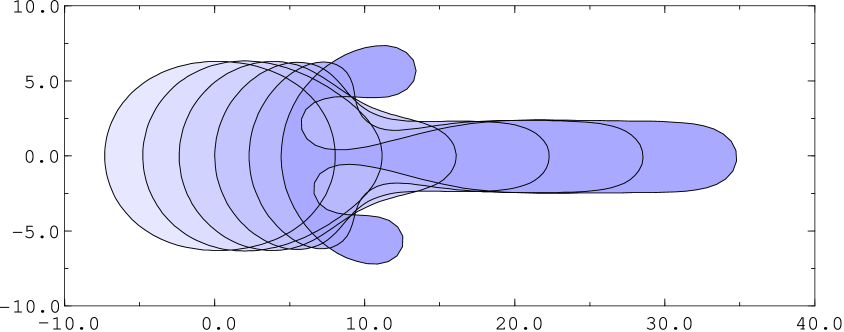
Figure 5. Breakup of an island in the isotropic case. The figure shows a time sequence of shapes, with a shading that darkens with increasing time. The initial shape is an ellipse elongated in the direction of island motion, with an area corresponding to a circle of dimensionless radius $\rho_{0}=7$. The computation used 150 discretization nodes. The breaking of the up-down symmetry is due to numerical noise.

To link our investigation to previous work we start with the isotropic case $S=0$. Here we find circular stationary solutions for small radii. At the critical dimensionless radius $\rho_{c}=3.26$ the circular solution loses its stability [19] and a bifurcation to non-circular stationary shapes occurs. In [30] this bifurcation was investigated by numerically solving the stationarity condition (3.1), and two branches of post-bifurcation shapes were found. In our time-dependent integration we only observe one branch, referred to as ‘mode I’ in [30]. To linear order in the distance from the bifurcation, the second ‘mode II’ branch is the symmetrical counterpart with respect to the circle, in the sense that $\kappa_{I}(\theta)+\kappa_{II}(\theta)=const.$; mode I is elongated in the direction of the field, mode II perpendicular to it. The mode II shapes which move at a smaller velocity seem not to be selected by the dynamics.

Some noncircular stationary shapes for $S=0$ are shown in Fig.4. We see that for $\rho_{0}\geq 3.5$ the shapes become non-convex. These shapes were not found in [30], because the numerical calculation was stopped at the point where $1/\kappa$ approaches zero. Increasing the dimensionless island size further above $\rho_{0}\simeq 6.2$ causes the island to break. It first evolves a long finger, which corresponds to the ‘slit’-solution described in [17], and which subsequently detaches to form a new island (Fig. 5). Similar breakups occur in the presence of anisotropy, so that the range of $\rho_{0}$ is generally restricted towards large values.

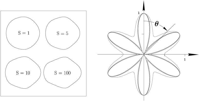
Figure 6. Left panel: Stationary shapes with anisotropic mobility of sixfold symmetry ($D=3$). The initial shape was a circle of dimensionless radius $\rho_{0}=2.5$, and the anisotropy strength is $S=1$, 5, 10 and 100. The computation used 50 discretization nodes. Right panel: Polar plot of the mobility corresponding to the shapes in the left panel.

For the anisotropic case there are no circular stationary shapes anymore. The deviation from the circle increases with increasing size $\rho_{0}$ and strength of anisotropy $S$. For strong anisotropy the islands evolve facet-like features, i.e. regions of the edge where the radius of curvature is very large. Figure 6 shows some examples. As was already discussed in Sect. 3.2, the direction of motion generally differs from the field direction, when the latter is not aligned with the symmetry axes of the anisotropy. Under certain conditions the symmetry of the direction of motion with respect to the field and anisotropy direction appears to be spontaneously broken, i.e. we have observed stationary island migration off the field direction even when the latter coincides with a symmetry axis of the anisotropy [33]. This behavior may be related to the discontinuity of the direction of motion when the field direction crosses the direction of minimal mobility, which was described in Sect.3.2 for the capillarity-free case.

With increasing $S$ the range of $\rho_{0}$ for which stationary solutions exist shrinks toward smaller values and is replaced by a domain where a qualitatively new behavior appears. Here the time evolution neither runs into a steady state nor into a breakup event but instead becomes oscillatory. A typical sequence is shown in Fig.7: First the island elongates along the field direction, then one side of it bends so that the conformation becomes nonconvex. This leads to an acceleration of the mass transport which then shrinks the shape back to its original state. The oscillatory shape evolution in Fig.7 is moreover seen to break the symmetry with respect to the field and anisotropy direction (recall that the field is directed along the $x$-axis which corresponds to a direction of maximal mobility, see the right panel in Fig.6). The solution shown in Fig.7 coexists with one obtained by reflection at the $x$-axis, in which the island travels to the right and down. Which of the two solutions is realized depends on the initial conditions. For other parameter values we have also observed solutions that switch between periods of upward and downward motion [33].

The conditions for the appearance of stationary and oscillatory shapes largely remain to be clarified. On a qualitative level, we have observed that the “facets” that dominate the stationary shapes for large $S$ tend to be close to orientations of maximal stability in the sense of linear stability analysis [34]. In contrast, the oscillatory shapes are typically bounded by one stable and one unstable orientation, and the shape oscillation can be viewed as the propagation of a wave along the unstable side of the island (see Fig.7).

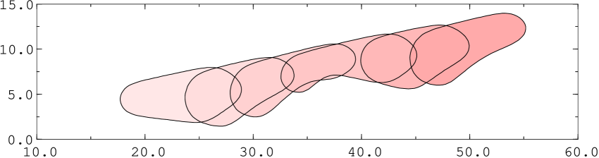
Figure 7. Oscillatory island motion. The dimensionless initial radius was $\rho_{0}=4$ and the anisotropy strength $S=1$. Note that the upper boundary is stable, while the lower boundary supports a traveling wave. The computation used 100 discretization nodes.

For the reasons described in Sect.3, a quantitative comparison between the shapes computed numerically for the full problem and the analytically derived capillarity-free shapes is not meaningful. On a qualitative level, the most apparent difference between the shapes in Fig.2 and Figs.4,6 is that in the presence of capillarity the direction of motion can clearly be discerned from the shape, while the capillarity-free shapes in Fig.2 are front/back symmetric. This can be seen directly from (3.1). If $\tilde{\gamma}=0$ the equation reduces to (again using $\frac{\partial}{\partial s}=\kappa\frac{\partial}{\partial\theta}$)

$$F\kappa\frac{d}{d\theta}\sigma(\theta)\cos(\theta+\phi)=V\sin(\theta)$$ (4.1)

which possesses two symmetries: First, reversing the direction of the field and the velocity simultaneously leaves the equation invariant. The second symmetry is the $\pi$-periodicity of the equation which results in periodicity of the solution. Both symmetries are destroyed for nonzero stiffness.

5. Conclusions

It is interesting to compare the local ($\Sigma^{\prime}/\Sigma=1$) and nonlocal ($\Sigma^{\prime}/\Sigma<1$) boundary evolution problems in the light of our work. For the isotropic case, it is known that the circular solution becomes linearly unstable for sufficiently large radius when $\Sigma^{\prime}/\Sigma>0$ [19], while it retains its stability (but becomes nonlinearly unstable under a sufficiently large perturbation [22, 27]) when $\Sigma^{\prime}/\Sigma=0$ [19, 20]. Furthermore it has been shown by complex variable techniques that noncircular stationary shapes cannot exist for $\Sigma^{\prime}/\Sigma=0$ [27], hence a void is forced to break up when it becomes unstable [22]. Here we have shown that breakup occurs for sufficiently large islands also in the local case, but in addition there is an intermediate regime, between the linear instability of the circular solution and breakup, where noncircular stationary solutions are stable.

Perhaps our most remarkable finding is that crystal anisotropy may induce complex, oscillatory evolution modes in the local problem. An example of oscillatory void evolution was previously reported by Gungor and Maroudas in the nonlocal case [36]. Future work should address the robustness and generality of the phenomenon. For this purpose it should be useful to employ numerical methods that are complementary to the sharp interface algorithm adopted here, such as finite element [21], phase-field [23, 26, 28], level set [24] and kinetic Monte Carlo [10, 13, 14] approaches, and to extend the study of the additional kinetic regimes (other than the case of edge diffusion considered here) in [10] to include crystal anisotropy.

References

- [1] C.V. Thompson, J.R. Lloyd, Electromigration and IC interconnects. MRS Bulletin 18, No.12 (1993), 19–25.
- [2] K.N. Tu, Recent advances on electromigration in very-large-scale-integration of interconnects. J. Appl. Phys. 94 (2003), 5451–5473.
- [3] Z. Suo, Reliability of Interconnect Structures. In: Comprehensive Structural Integrity, I. Milne, R.O. Ritchie, B. Karihaloo, Editors-in-Chief, Vol. 8: Interfacial and Nanoscale Failure, W. Gerberich, W. Yang, Editors (Elsevier, Amsterdam 2003), 265–324.
- [4] E. Arzt, O. Kraft, W.D. Nix, J.E. Sanchez, Jr., Electromigration failure by shape change of voids in bamboo lines. J. Appl. Phys. 76 (1994), 1563–1571.
- [5] O. Kraft, Untersuchung und Modellierung der Elektromigrationsschädigung in miniaturisierten Aluminiumleiterbahnen. PhD Dissertation (University of Stuttgart, 1995).
- [6] Y.-C. Joo, S.P. Baker, E. Arzt, Electromigration in single-crystal aluminum lines with fast diffusion paths made by nanoindentation. Acta Mater. 46 (1998) 1969–1979.
- [7] M.R. Gungor, D. Maroudas, Theoretical analysis of electromigration-induced failure of metallic thin films due to transgranular void propagation. J. Appl. Phys. 85 (1999) 2233–2246.
- [8] A.H. Verbruggen, Fundamental questions in the theory of electromigration. IBM J. Res. Develop. 32 (1988) 93–98.
- [9] R.S. Sorbello, Theory of electromigration. Solid State Phys. 51 (1998), 159–231.
- [10] O. Pierre-Louis, T.L. Einstein, Electromigration of single-layer clusters. Phys. Rev. B 62 (2000) 13697–13706.
- [11] J.-J. Métois, J.C. Heyraud, A. Pimpinelli, Steady-state motion of silicon islands driven by a DC current. Surf. Sci. 420 (1999), 250–258.
- [12] A. Saúl, J.-J. Métois, A. Ranguis, Experimental evidence for an Ehrlich-Schwoebel effect on Si(111). Phys. Rev. B 65 (2002) 075409.
- [13] H. Mehl, O. Biham, O. Millo, M. Karimi, Electromigration-induced flow of islands and voids on the Cu(100) surface. Phys. Rev. B 61 (2000), 4975–4982.
- [14] P.J. Rous, Theory of surface electromigration on heterogeneous metal surfaces. Appl. Surf. Sci. 175-176 (2001) 212–217.
- [15] J. Krug, Introduction to Step Dynamics (this volume).
- [16] M. Schimschak and J. Krug, Electromigration-driven shape evolution of two-dimensional voids. J. Appl. Phys. 87 (2000) 695–703.
- [17] Z. Suo, W. Wang and M. Yang, Electromigration instabilities: transgranular slits in interconnects. Appl. Phys. Lett. 64 (1994) 1944–1946.
- [18] P.S. Ho, Motion of an inclusion induced by a direct current and a temperature gradient. J. Appl. Phys. 41 (1970) 64–68.
- [19] W. Wang, Z. Suo, T.-H.Hao, A simulation of electromigration-induced transgranular slits. J. Appl. Phys. 79 (1996) 2394–2403.
- [20] M. Mahadevan, R.M. Bradley, Stability of a circular void in a passivated, current-carrying metal film. J. Appl. Phys. 79 (1996), 6840–6847.
- [21] L. Xia, A.F. Bower, Z. Suo, C.F. Shih, A finite element analysis of the motion and evolution of voids due to strain and electromigration induced surface diffusion. J. Mech. Phys. Solids 45 (1997) 1473–1493.
- [22] M. Schimschak, J. Krug, Electromigration-Induced Breakup of Two-Dimensional Voids. Phys. Rev. Lett. 80 (1998) 1674–1677.
- [23] M. Mahadevan, R.M. Bradley, Simulations and theory of electromigration-induced slit formation in unpassivated single-crystal metal lines. Phys. Rev. B 59 (1999), 11037–11046.
- [24] Z. Li, H. Zhao, H. Gao, A Numerical Study of Electro-migration Voiding by Evolving Level Set Functions on a Fixed Cartesian Grid. J. Comp. Phys. 152 (1999), 281–304.
- [25] M. Ben Amar, L.J. Cummings, G. Richardson, A theoretical treatment of void electromigration in the strip geometry. Comp. Mater. Sci. 17 (2000), 279–289.
- [26] D.N. Bhate, A. Kumar, A.F. Bower, Diffuse interface model for electromigration and stress voiding. J. Appl. Phys. 87 (2000) 1712–1721.
- [27] L.J. Cummings, G. Richardson, M. Ben Amar, Models of void electromigration. Eur. J. Appl. Math. 12 (2001), 97–134.
- [28] J.H. Kim, P.R. Cha, D.H. Yeon, J.K. Yoon, A phase field model for electromigration-induced surface evolution. Metals and Materials International 9 (2003), 279–286.
- [29] Z. Suo, Electromigration-induced dislocation climb and multiplication in conducting lines. Acta metall. mater. 42 (1994), 3581–3588.
- [30] W. Yang, W. Wang, Z. Suo, Cavity and dislocation instability due to electric current. J. Mech. Phys. Solids 42 (1994) 897–911.
- [31] M. Schimschak, Numerische Untersuchungen zur Elektromigration auf metallischen Oberflächen, PhD Dissertation (University of Essen, 1999).
- [32] L.F. Shampine, M.K. Gordon, Computer Solution of Ordinary Differential Equations – The Initial Value Problem (W.H. Freeman, San Francisco, 1975).
- [33] P. Kuhn, J. Krug (in preparation).
- [34] J. Krug, H.T. Dobbs, Current-Induced Faceting of Crystal Surfaces. Phys. Rev. Lett. 73 (1994), 1947–1950.
- [35] M. Schimschak, J. Krug, Surface Electromigration as a Moving Boundary Value Problem. Phys. Rev. Lett. 78 (1997), 278–281.
- [36] M.R. Gungor, D. Maroudas, Current-induced non-linear dynamics of voids in metallic thin films: morphological transition and surface wave propagation. Surf. Sci. 461 (2000), L550–L556.
Acknowledgment
We would like to thank Martin Schimschak for helpful correspondence.