Modifications and Extensions to Harrison’s Tight-Binding Theory

Abstract

Harrison’s tight-binding theory provides an excellent qualitative description of the electronic structure of the elements across the periodic table. However, the resulting band structures are in significant disagreement with those found by standard methods,particularly for the transition metals. For these systems we developed a new procedure to generate both the prefactors of Harrison’s hopping parameters and the onsite energies. Our approach gives an impressive improvement and puts Harrison’s theory on a quantitative basis. Our method retains the most attractive aspect of the theory, in using a revised set of universal prefactors for the hopping integrals. In addition, a new form of onsite parameters allows us to describe the lattice constant dependence of the bands and the total energy, predicting the correct ground state for all transition, alkaline earth and noble metals. This work represents not only a useful computational tool but also an important pedagogical enhancement for Harrison’s books.

I Introduction

Walter Harrison developed an elegant analytic theory of the electronic structure of solids har_book_80 ; har_book_99 . This theory has been very sucessful in providing a physical understanding of the electronic structure and the characteristics of bonding. However, Harrison’s theory of solid state has limited ability to produce accurate numerical results for the band structure, density of states and the relative stability of different crystal structures.

In this work, we have set out to put Harrison’s approach on a quantitative foundation. We have now realized that it is possible to put the Slater-Koster parameters in the form given by Harrison but with new prefactors and determine new onsite parameters. The result is that we retain the universality of Harrison’s parameters, which means the same prefactors for all transition,alkaline earth and noble metals, but with different onsite terms for each element. It is clear to us that this approach,perhaps slightly modified,may be extended to cover the rest of the periodic table. We have also succeeded with a small number of additional parameters to describe the volume and structure dependence of the energy bands and, therefore, obtain total energies and predictions of relative stability.

Harrison has opted for simplicity in the LCAO approach and has created a set of universal hopping parameters that can easily be used to perform calculations. In the tables of his books,Harrison uses atomic energies as onsite parameters in his Hamiltonians, which is the main shortcoming of directly using these tables, to perform sufficiently accurate band structure calculations. However,Harrison pointed out(har_book_99 ,p561) that atomic values for the d-state energies need to be corrected for differences in d-state occupancy, and gave a way for doing that in the case of Cr.

We illustrate the importance of correcting the values of the onsite parameters for the transition metals Nb and Pd by using Harrison’s hopping parameters and uncorrected atomic term values. We compared the results of a $6\times 6$ Harrison Hamiltonian(without $p$ orbitals) as given in Harrison’s book and we found that the energy bands created this way are in serious disagreement with Augmented Plane Wave(APW) results (see left Fig. 1). We also tested a $9\times 9$(with $p$ orbitals) Harrison Hamiltonian with all hopping prefactors kept at Harrison’s values, but the onsite parameters modified by fitting the energy bands to APW calculations. Sigalas ; papa This modification gave us better results in the $d-$bands, but there was still a large error for the s-like first band(see right Fig. 1). Our conclusion is that Harrison’s theory can only give a qualitative description of the band structure of the transition metals even if we fit the onsite terms to first-principles results.

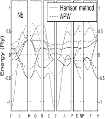
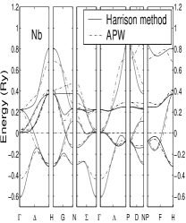
Figure 1: Harrison’s energy bands of Nb compared to APW. Left graph created by $6\times 6$ Hamiltonian; right graph created by $9\times 9$ Hamiltonian and fitted onsite energies.

II Energy Bands and Density of States

We have developed a procedure that while maintaining the simplicity of Harrison’s approach gives an impressive improvement that puts the theory on a quantitative basis. To accomplish this we have made the following modifications to Harrison’s theory: (1) We introduced a $p$ onsite energy as an additional parameter to the $s$ and $d$ onsite energies used by Harrison, and fit them all to APW results. (2) We modified the $sp$ hopping integrals of Harrison, by introducing a dimensionless parameter $\gamma_{s}$ as follows:

$$V_{ll^{\prime}m}=\eta_{ll^{\prime}m}\frac{\gamma_{s}\hbar^{2}}{m_{e}d^{2}}$$ (1)

The parameter $\gamma_{s}$ provides more flexibility to fit the first and sixth bands. (3) We obtained new hopping prefactors by simultaneously fitting the APW energy bands of the following 12 transition metals: V, Cr, Ni, Cu, Nb, Mo, Pd, Ag, Ta, W, Pt and Au. In this fit, all 12 elements have the same common prefactors $\eta_{ll^{\prime}m}$ but different(for each element) onsite energies s, p and d, and also different values for the parameters $\gamma_{s}$ and $r_{d}$ that appear in the hopping parameters. Our Hamiltonian corresponds to an orthognal basis set as in Harrison. We did the above fitting at the equilibrium lattice constants of the structure, which is the ground state of each element, and included interactions of nearest, second-nearest, and third-nearest neighbors for the $bcc$ structure and nearest and second-nearest for the $fcc$ structure. Of course, using more neighbors than Harrison did in the fit would automatically make changes in the parameters, even if one were fitting the same bands. Using the parameters determined with the above procedure, we reproduced APW energy bands and density of states(DOS) remarkably well, not only for the 12 elements originally fitted, but also for the rest of the transition metals, the alkaline earth and the noble metals, as seen in Fig. 3 and Fig. 3 for four of the elements. Our new Hamiltonian prefactors, common for all metals, together with Harrison’s original prefactors are shown in Table 1. The onsite terms and the parameters $\gamma_{s}$ and $r_{d}$ for each element are shown in Table 2.

Table 1: Harrison’s hopping prefactors and our modified values.

	$\eta_{ss\sigma}$	$\eta_{sp\sigma}$	$\eta_{pp\sigma}$	$\eta_{pp\pi}$	$\eta_{sd\sigma}$
Harrison	-1.32	1.42	2.22	-0.63	-3.16
Modified Harrison	-0.90	1.44	2.19	-0.03	-3.12
	$\eta_{pd\sigma}$	$\eta_{pd\pi}$	$\eta_{dd\sigma}$	$\eta_{dd\pi}$	$\eta_{dd\delta}$
Harrison	-2.95	1.36	-16.2	8.75	-2.39
Modified Harrison	-4.26	2.08	-21.22	12.60	-2.29

Table 2: Onsite parameters, $\gamma_{s}$ and $r_{d}$.

Name	$s(Ry)$	$p(Ry)$	$d(Ry)$	$\gamma_{s}$	$r_{d}(a.u.)$
K	0.26067	0.22200	0.25426	1.13081	3.65981
Ca	0.11994	0.24522	0.03657	1.07535	2.66618
Sc	0.14809	0.38903	-0.06695	0.98860	2.12358
Ti	0.51352	0.79759	0.21879	0.92307	1.85267
V	0.64331	0.73136	0.04711	0.90164	1.65358
Cr	0.76372	0.86088	0.06389	0.87733	1.51087
Mn	0.47377	0.86874	-0.00300	0.82491	1.42366
Cu	0.54432	0.93013	-0.05425	0.92178	1.23548
Zn	0.44779	0.77968	-0.10598	0.78430	0.97054
Sr	0.32339	0.41296	0.22810	1.22463	3.29024
Y	0.29652	0.51778	-0.07450	1.19367	2.75073
Zr	0.54322	0.87432	0.17820	1.15726	2.40732
Nb	0.85097	0.99247	0.24572	1.08802	2.19244
Mo	0.83057	0.97345	0.10805	1.06314	2.01708
Tc	0.64629	1.08072	0.09302	1.00014	1.91300
Ru	0.65130	1.07465	0.04760	1.00001	1.80799
Rh	0.68579	1.06923	0.06445	0.99989	1.71702
Pd	0.57192	0.95218	0.04268	0.90172	1.63401
Ag	0.44541	0.79565	-0.04959	0.84306	1.52479
Ba	-0.04951	0.03502	-0.20497	1.07269	3.56198
Hf	0.29999	0.75423	0.32239	0.88204	2.50856
Ta	0.70455	0.92990	0.23577	1.12532	2.31790
W	0.64038	0.86882	0.09170	1.11008	2.17888
Re	0.60996	1.15988	0.15348	1.14822	2.08878
Os	0.53044	1.06428	0.05117	1.11453	2.01287
Ir	0.47125	1.01759	0.01404	1.06585	1.91597
Pt	0.43374	0.94903	0.00569	1.00933	1.83802
Au	0.37521	0.84519	-0.02211	0.94002	1.75060
Hg	0.36137	0.68747	-0.10952	0.90569	1.53337
Fe	0.87761	0.84369	0.02940	0.94826	1.33156
Fe	0.84395	0.88024	0.19670	0.93012	1.43124
Ni	0.45155	0.69040	-0.04560	0.72937	1.22004
Ni	0.46394	0.70316	-0.00173	0.73568	1.24548
Co	0.69846	0.68425	-0.06187	0.79695	1.26137
Co	0.66026	0.70002	0.06184	0.77917	1.33184

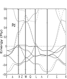
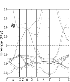
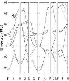
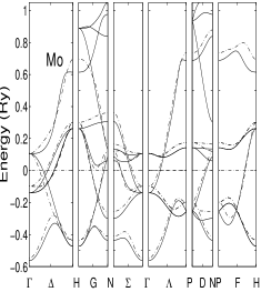
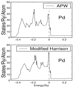
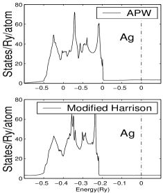
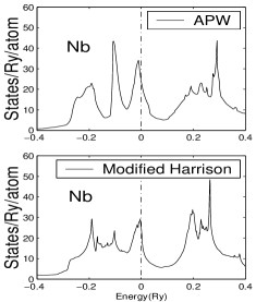
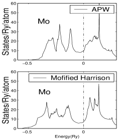
Figure 2: APW and Modified Harrison’s energy bands of Ag, Pd, Nb and Mo. The solid line is the modified Harrison result and dash-dotted line is the APW result.

Figure 3: APW and Modified Harrison’s density of states of Ag, Pd, Nb and Mo.

We used the prefactors of Table 1 with new onsite energies $\gamma_{s}$ and $r_{d}$ to fit the rest of the transition metals, including those with hcp ground states. For the hcp metals, we fitted energy bands of fcc structures at the equilibrium lattice, and found that our parameters produce good transferability, ie. reproduced the hcp energy bands very well without fitting them. The hcp energy bands of Ti and Ru are shown in Fig. 4. We also fitted energy bands of the ferromagnetic elements Fe, Co and Ni, and calculated magnetic moments of the three elements at the experimental lattice constant. Table 3 shows good agreement of magnetic moments of Fe, Co and Ni with experimental values.

Table 3: Magnetic Moments of Fe, Co and Ni.

Element	Structure	TB($\mu_{B}$)	Exp.($\mu_{B}$)
Fe	bcc	2.21	2.22
Co	hcp	1.52	1.72
Ni	fcc	0.56	0.61

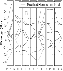
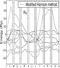
Figure 4: Energy bands of hcp Ti and Ru.

III Total Energy

Next we address the issue of fitting total energy results. In order to do this we follow the Naval Research Laboratory tight-binding(NRL-TB) methodology NRL-TB ; NRL-review , which uses parameters which are transferable between structures NRL-TB . In most TB approaches as well as in all the so-called “glue” potential atomistic methods one writes the total energy as a sum of a band energy term( sum of eigenvalues) and a repulsive potential $G[n(r)]$ that can be viewed as replacing all the charge density $n(r)$ dependent terms appearing in the total energy expression of the density functional theory. The NRL-TB method has the unique feature that eliminates G by the following ansatz. We define a quantity $V_{0}$:

$$V_{0}=\frac{G[n(r)]}{N_{e}}$$ (2)

where $N_{e}$ is the number of valence electrons.

We then shift all first-principles eigenvalues $\epsilon_{i}(k)$ by the constant $V_{0}$ and define a shifted eigenvalue:

$$\epsilon_{i}^{\prime}(k)=\epsilon_{i}(k)+V_{0}$$ (3)

The results of this manipulation is that the first-principles total energy $E$ is given by the expression:

$$E=\Sigma\epsilon_{i}^{\prime}(k)$$ (4)

We note the constant $V_{0}$ is different for each volume and structure of the first-principles database. The reader should recognize that we have shifted each band structure by a constant, retaining the exact shape of the first-principles bands. It should also be stressed that all this is done to the first-principles database before we proceed with the fit that will generate the TB Hamiltonian. In our trearment of ferromagnetic systems the total energy is equal to the sum of spin up and spin down shifted eigenvalues. The difference of these two sums could be viewed as representing the exchange energy.

We write the onsite energies in a polynomial form:

$$h_{il}(\rho_{i})=\alpha_{l}+\beta_{l}\rho^{\frac{2}{3}}_{i}+\gamma_{l}\rho^{\frac{4}{3}}_{i}+\delta_{l}\rho^{2}_{i}$$ (5)

where $l$ is an angular momentum index, and $\rho_{i}$ is an atomic-like density that has the form:

$$\rho_{i}=\sum_{j\neq i}exp[-\lambda^{2}R_{ij}]F_{c}(R_{ij})$$ (6)

where, $R_{ij}$ is the distance between atom i and j, and $F_{c}$ is a smooth cut-off function that was used to limit the range of parameters NRL-TB

$$F_{c}(R)=(1+e^{\frac{R-R_{0}}{R_{l}}})^{-1}$$ (7)

We take $R_{0}$ to be in the range of $10.0a_{0}\sim 14.0a_{0}$, and $R_{l}=0.5a_{0}$ ( where $a_{0}$ is Bohr radius), which effectively zeros all interactions for neighbors more than $14.0a_{0}$ apart. Typically, depending on the structure and lattice constant, this cut-off function will include $50\sim 80$ neighboring atoms.

The parameters $\lambda$, $\alpha_{l}$, $\beta_{l}$, $\gamma_{l}$ and $\delta_{l}$ are determined by fitting total energies following the NRL-TB procedure as stated above. The hopping parameters were calculated using the modified prefactors of Table 1.

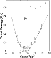
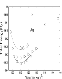
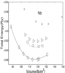
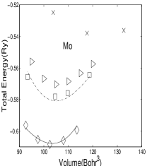
Figure 5: Total energies of Ag, Pd, Nb and Mo. The solid line denotes bcc APW results and dash-dotted line denotes fcc APW results. The diamond, square, triangle and X symbols represent bcc, fcc, hcp and sc TB results respectively.

We fitted total energies of all transition metals to the APW results Sigalas at several lattice constants of bcc, fcc and sc structures. We successfully reproduced the ground-state, the order of crystal structures and the bulk modulus. Our parameters also place the energies of hcp and sc structures, which we did not fit, at reasonable values. As an example, we present energy-volume relationships for four transition metals in Fig. 5, and for the hcp metals Ti and Co in Fig. 6, which again show the correct ordering of crystal structures. We also present in Table 4 the equilibrium lattice constants and bulk moduli of transition metals.

An inspection of Table 4 reveals that our approach matches very well the LDA lattice constants underestimating the experimental values by $1\--2\%$ for the transition metals and by $4\--5\%$ for the alkaline earths. The bulk moduli have larger deviation from experiment as is usually the case in the LDA. For the hcp metals both the lattice parameters and bulk moduli are also within the LDA predictions except for Tc, Os and Y. Those results could be improved if we include the hcp lattice in the fitting database.

Table 4: Equilibrium lattice constants and bulk moduli for the experimentally Kittel observed ground-state structures of the elements, comparing the results of first-principles and tight-binding parametrization results.

		a(Bohr)			$B_{0}(Mbar)$
Name	Structure	TB	LDA	Expt.	TB	LDA	Expt.
Ca	fcc	9.98	9.96	10.55	0.21	0.13	0.15
V	bcc	5.55	5.54	5.73	2.15	1.96	1.62
Cr	bcc	5.29	5.29	5.44	3.05	3.07	1.90
Fe	bcc	5.38	5.38	5.43	1.76	1.76	1.68
Ni	fcc	6.48	6.48	6.65	2.38	2.52	1.86
Cu	fcc	6.71	6.65	6.82	2.01	1.90	1.37
Sr	fcc	10.94	10.82	11.49	0.11	0.20	0.11
Nb	bcc	6.16	6.16	6.24	1.93	1.95	1.70
Mo	bcc	5.91	5.90	5.95	2.98	2.91	2.72
Rh	fcc	7.11	7.12	7.18	3.87	3.22	2.70
Pd	fcc	7.34	7.29	7.35	1.93	1.84	1.81
Ag	fcc	7.62	7.58	7.73	1.32	1.16	1.01
Ba	bcc	9.02	9.03	9.49	0.17	0.10	0.10
Ta	bcc	6.22	6.12	6.24	2.12	2.24	2.00
W	bcc	5.99	5.94	5.97	3.63	3.33	3.23
Ir	fcc	7.30	7.29	7.26	4.14	3.86	3.55
Pt	fcc	7.43	7.37	7.41	3.34	3.05	2.78
Au	fcc	7.77	7.67	7.71	1.87	1.70	1.73
		a(Bohr)		c(Bohr)		$B_{0}(Mbar)$
Name	Structure	TB	Expt.	TB	Expt.	TB	Expt.
Sc	hcp	5.98	6.25	9.55	9.96	0.34	0.44
Ti	hcp	5.54	5.58	8.81	8.85	1.17	1.05
Co	hcp	4.74	4.74	7.70	7.69	2.35	1.91
Y	hcp	6.58	6.90	10.62	10.83	0.70	0.37
Zr	hcp	5.95	6.11	9.52	9.74	0.87	0.83
Tc	hcp	5.12	5.18	8.38	8.31	5.42	2.97
Ru	hcp	5.10	5.12	7.70	8.09	3.52	3.21
Hf	hcp	6.05	6.03	9.13	9.54	1.06	1.09
Re	hcp	5.21	5.22	8.64	8.43	4.23	3.72
Os	hcp	5.28	5.17	7.61	8.16	6.98	4.18

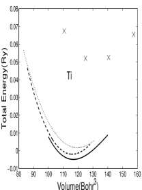
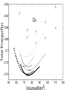
Figure 6: TB total energies of Ti and Co. The solid line, dotted line and dashed line represent hcp, bcc and fcc total energies respectively. The symbol + denotes simple cubic total energy. In the right graph, the thick lines and thin lines represent ferromagnetic and paramagnetic Co, and the symbols X and + show ferromagnetic and paramagnetic simple cubic respectively.

IV Conclusion

To recapitulate, we have accomplished two goals. In the first we have reevaluated the ten universal prefactors in Harrison’s hopping parameters and redetermined the $s,p,d$ onsite energies together with the parameters $\gamma_{s}$ and $r_{d}$. This enables us to calculate very accurately the band structure of all the transition, alkaline earth and noble metals. For the second goal we have used a polynomial form for the onsite energies which, with the addition of 15 new parameters, provides a total energy capability for our Modified Harrison theory.

Finally, we wish to stress that this work constitutes not only an efficient computational method but also a valuable addendum to Harrison’s books.

Acknowledgment: We wish to thank Professor Walter A. Harrison and Drs Michael J. Mehl and Larry L. Boyer for valuable comments.

References

- (1) Walter A. Harrison, Electronic Structure and Properties of Solids, Dover, (1980).
- (2) Walter A. Harrison, Elementary Electronic Structure, World Scientific, (1999).
- (3) M. Sigalas, D.A. Papaconstantopoulos and N.C. Bacalis, Phys. Rev. B 45, 5777 (1992).
- (4) D.A. Papaconstantopoulos, Handbook of the Band Structure of Elemental Solids, Plenum Press, (1986).
- (5) M. J. Mehl and D. A. Papaconstantopoulos, Phys. Rev. B 54, 4519-30 (1996).
- (6) D.A.Papaconstantopoulos and M. J. Mehl, J. Phys.: Condens. Matter 15, 413-440 (2003).Review
- (7) C. Kittel, Introduction to Solid State Physics, Wiley, (1953).