Comparison of social and physical free
energies on a toy model

Abstract

Social free energy has been recently introduced as a measure of social action obtainable in a given social system, without changes in its structure. The authors of this paper argue that social free energy surpasses the gap between the verbally formulated value sets of social systems and the quantitatively based predictions. This point is further developed by analyzing the relation between the social and the physical free energy. Generically, this is done for a particular type of social dynamics. The extracted type of social dynamics is one of many realistic types of the differing proportion of social and economic elements. Numerically, this has been done for a toy model of interacting agents. The values of the social and physical free energies are, within the numerical accuracy, equivalent in the class of non-trivial, quasi-stationary model states.

I Introduction

The modelling of social systems based on notions from statistical physics enriches the understanding of collective phenomena [M22, - M24, ]. Within that context the social meaning of free energy has been explicitly addressed [M22, - M5, ]. Social free energy was introduced as a measure of system resources which are unused in regular, predicted functioning, but which are involved during suppression of environmentally induced dynamics changes M5 . Depending on the context, it was recognized as the combination of innovation and conformity of a collective [M22, - M24, ], profit M1 , common benefit M2 , availability M3 , or free value of the canonical portfolio M4 . The free energy in the references listed was introduced at the quantitative level in the usual way (expression (9) in this article) and was linked with its sociological interpretation. The listed social interpretations of the physical free energy imply existence of a socially relevant quantity, analogue or at least closely related to physical free energy. However, the very diversity of the notions and their independent development show that a unified approach to recognizing social meaning of the physical free energy is still missing.

This paper claims that social situations are interpreted (e.g., present situations described and future predicted) based on evaluation of a social analogue of physical free energy.

The development of the social interpretation of the free energy is by no means straightforward, as it invokes calculations in the social, predominantly verbally formulated context. The following scheme of the development is suggested: (i) contextualization of the free energy, (ii) definition of the interacting agent toy model in the context set, (iii) independent introduction of social free energy and physical free energy within the model (the former quantity is introduced from strictly qualitative, readily recognizable considerations as the measure of particular social action, while the latter is calculated using the well-founded formalism of statistical mechanics, seemingly unrelated to the social context of the model), (iv) calculation of these two quantities for evolving state of the interacting agent toy model, and a posteriori demonstration of the validity of the initial claim for the model. This equality is the starting point for further, more profiled analyses of relation between the two types of free energies. Clear relation between the social and physical free energy would provide one with a broadly applicable quantitative mean for analysis of social systems’ aggregated quantities, which in turn contributes to better understanding of the social system dynamics. In this sense we emphasize the quantification of social context, as it has been rather vaguely covered in the literature in comparison with the economic one. In addition, we do not attempt to simplify the entire existing social and economic dynamics to one simple model. Instead, among the large number of existing types of social system dynamics we concentrate on one particular type, apply the stated scheme onto it, and subsequently model it. Still, we consider the defining of social free energy, and the establishing of its relation with physical free energy to be independent of the particular represented type of the social system dynamics.

The paper is organized as follows. The social context of social system dynamics is discussed in the second section in order to elaborate the link between the general social system and its projection on the quantifiable subsystem. The toy model corresponding to a particular social behavior is described in the third section. The model indicators are introduced in the fourth section. Results of calculations of free energies are discussed in the fifth section. The main results are summarized in the sixth section.

II Basic elements of social system value set

A value set is a qualitative structure attributed to a social system, which collects formal (legislative) and informal (customs, norms and values) rules governing complete social dynamics of a social system. It is a fact of life that value sets differ significantly. The interpretation of many types of transfer of tradable goods, some of these being seemingly strictly economic, requires the full value set of the corresponding social system. Let us illustrate this by using the following two examples.

The first example is ”the Melanesian culture of status-seeking through gift giving. Making a large gift is a bid for social dominance in everyday life in these societies, and rejecting the gift is a rejection of being subordinate.” [M6, , p.159]. Gifts in that culture combine the economic context of what is otherwise a valuable collection of resources with the social one. In the ultimatum game experiment (described in detail by Gintis M6 ) in which participants pair-wisely arrange transfer of resources they are initially given, on average participants belonging to such a culture ”offered more than half pie, and many of these ’hyperfair’ offers were rejected.” M6 . In contrast, the fair transfer within market trading economy is considered to be the half pie.

The second example is the potlatch, the ritualized barter ceremony often used to settle positions in communities of North American Indians. ”A person’s prestige depended largely on his power to influence others through impressive size of gifts offered, and, since the debts carried interest, the ’giver’ rose in the eyes of the community to be …a person of considerable standing.” [M7, a]. Valuable resources were even destroyed in order to demonstrate the owner’s wealth and prestige [M7, b].

These examples illustrate the point that the realistic collective behavior incorporates a large number of types, some of which are unrealistic if interpreted by different value sets. Taking these diverse systems mutually on equal footing is useful in gaining understanding of generic system quantities. Before proceeding, let us stress these points, because a reduction of value sets, needed for the sake of operationality, suppresses the social context and leaves rather unrealistic behavior.

Despite the recognized importance of value sets in regulating social dynamics, these constructs have been rarely linked in detail. As an illustration, altruism and self-interest as two of human characteristics are incorporated in diverse value sets with different significance. However, their precise meaning is still missing. Regarding this, recent literature points out that the understanding of altruism is still changing significantly, which includes the recognition of its sub-categories [M8, , M9, ]. On the other hand, the boundary between self-interest and altruism is questionable. The interpretation of other human-related terms is similarly unsettled. All this influences the interpretation of social dynamics and its derivatives, e.g. simulation models.

As a consequence, for the sake of a definite interpretation of simulation results, one needs to reduce the complexity of social dynamics through its relation to quantifiable resources. The reduction of social dynamics requires the reduction of the corresponding value set. Reduction implies extracting the facts, regarding observable actions which include resources, from the value sets. The set of thus extracted facts does not belong to any particular social system. Yet, its representative quality is sufficient to justify its broadening and linking to a specific system.

In this way, a prerequisite for determining the relation between the social and physical free energy is formulated. Such a relation contributes to simplifying the rules of social dynamics. Furthermore, it contributes to the importance of existing formalism of physics in the relatively new context.

The resources are quantifiable artifacts, objects, materials and human characteristics (e.g. free time, skills, knowledge) linked to social dynamics. The use of resources spans the range from economic to social, as illustrated previously. Let us use the following three types of resources, in which the proportion of social context is prevalent or at least significant, to contribute to the awareness of the importance of the socially-governed transfers: (i) grants, writing off debts (which occurs from individual to international level), money donations, etc., (ii) donated blood, and (iii) socially responsible investments and resources of charitable organizations (e.g. Salvation Army).

The processes including the listed types of resources share some elements; e.g. the donated blood is a regularly observed gift M10 . Blood donation

1. has significant impact on the individuals and the whole collective,

2. is strictly voluntary in the sense that there are no laws and penalties for potential blood donors who do not donate blood, and

3. relies heavily on the presumed honesty and sincerity of the giver, despite the observed fallacies.

Therefore, blood donation itself is related presumably to the part of the social system’s value set which is separated from economics. The extracted three points have been observed similarly in the cases of other listed types of resources.

The common points in the transfer of different resource types can be generalized: locally, there is non-homogeneous distribution of resources. A part of the population experiences a lack, and the other part a surplus of these. These conditions may be temporary or permanent, adopted by the majority or a minority of population. It is a fact that there are different processes which tend to balance the non-homogeneity of resource distribution (along with others which try to enhance the differences). These processes may be complexly structured (supported loans which require proofs of social status, and which are given in several time-separated phases), they may be permanent (blood donation), triggered by some event (help provided to people suffering from some natural disaster), combined (donations), with or without institutions mediating transfer of resources. These processes may be the consequences of the fact that resources given to the people who suffer from the lack of them eventually enable further collecting of the resources from the people with current surplus, or the consequences of socially responsible investments. They may be the consequences of philanthropic character of individuals with surplus of resources, or of their tendency to rise in the eyes of local population, i.e. to make their social rank higher, and augment the power which is related to the rank in the corresponding social system. They are usually sensitive to some characteristics of persons lacking resources, e.g., grants include citizenship or age requirements, grants are given only to some professions, help is given to neighbors, elderly, homeless, etc. On the average, however, most of the population lacking resources is eligible at least for some of the resource transfer processes. Aside from that, resource transfers tend to be localized in physical space, because the durability of resources, administrative requirements, etc. raise cost of or otherwise complicate the longer distance transfers. Moreover, there are fewer types of resources shared by the dynamics of more distant social systems.

As long as one is interested only in observable and quantifiable part of the processes of the types mentioned, the value sets’ related points should be suppressed. Thus one ends with the following rule expressing all relevant elements of the resource transfer:

part of resources is transferred from people with surplus
of resources to the neighboring people lacking resources

Before proceeding, the following point should be emphasized once again: the rule stated is not appropriate for all the existing resource transfers, e.g., for processes in market economies. It is appropriate for situations in which social dimension of processes is important, and expresses directly quantifiable part, which is linked by the value set to the other, directly non-quantifiable part. The exclusion of the value set includes the refraining from interpretation about persons giving part of resources, i.e., whether they are altruists or self-interested.

III Model

The model includes mutually interacting agents, their configuration and environmental impact.

Agents are fixed at nodes of two-dimensional net of dimensions $N_{0}\times N_{0}$, Fig. 1. Coordinates of agent on the $i$-th node in one direction and the $j$-th node in the other direction are denoted as $m=(i,j)$. Such a net, generally represents connections among agents. Hence it refers to socio-biological, economical relations, or relations caused by other interests among the agents. In some special cases it may refer to physical space occupied by agents. This point is addressed in more detail at the end of this section. Agents collect the resource $u$, a scalar quantity, which is taken to be a non-negative quantity. The amount of resources owned is a positive number or zero. An agent with resources $u$ is considered rich if $u>u_{0}$, poor if $u_{0}>u>0$, and dead if $u=0$. In the context of the model the terms rich and poor refer to the quantity of resources. In some special cases (donations, grants, etc.) they coincide with their conventional economic meaning. If resources of a particular agent become negative at some point of time, they are set to zero and the agent is considered dead. Dead agents are further excluded from the resource transfers. For a rich agent with resources $u$ the difference $u-u_{0}$ is called surplus of resources. Similarly, for a poor agent with resources $u$, the difference $u_{0}-u$ is called lack of resources. Let us remark that our model can also describe the systems with different types of resources if a fixed exchange ratio to a scalar quantity $u$ is defined for each type of resources.

As a consequence of internal, otherwise unspecified dynamics, agents regularly consume a finite value of resources $c$.

Because of the environmental influence, each agent’s resources are synchronously changed for a random amount $w(m)$. The distribution of changes $w$ is the Gaussian distribution with a mean value $a$ and a variance $\mu$ . The mean value $a$ represents the average resource change, and for a system we take $a>0$. In each time interval there are some resources obtained from the environment, and some resources destroyed because of the influences from the environment. If resources are smaller after the interaction with the environment this means that destructive influences, e.g., fire or flood, were stronger than the effects of making the resources larger. The choice of a symmetrical function for distribution of $w$ seemingly contradicts the usual skew shape of resource distributions M11 . However, since the positive (negative) part of the Gaussian distribution represents the increasing (reducing) the resources, it qualitatively collects the total interaction of the agents with the environment.

Such a setup of the model includes the relevant agent characteristics, in accordance with the definitions of the agent [M12, , M13, ], and the social agent M14 . Each agent acts on himself or herself, which is taken into account by the parameter $c$, and interacts with the environment, which is included through $a$ and $\mu$. The agents respond to the current environment state optimally in the sense that all agents always follow all the system rules which, nevertheless, does not assure them a sufficient amount of resources. Formally, this assures the equality of the form of distribution function for all agents. Owing to the simplicity of the toy model, the agent and the environment characteristics are somewhat mixed. On the one hand, the model covers the case of agents of bounded rationality, which share knowledge about environment, but the knowledge which does not include all the rules underlying environment dynamics. On the other hand, the agents in the model could have maximal possible knowledge about environment dynamics, but in the environment which itself is stochastic. In that sense, the optimal agent response means that in the system there are no local fluctuations of knowledge, i.e., all agents have identical knowledge about the environment and the processes of transfer of resources from the environment. In addition, it is further assumed that agents know exactly the local amount of resources. Further in the text the last assumption is included into the rule of intra-agent resource transfer in which resources of several neighboring agents are related.

The constancy of the parameters in space means that the system latency and integrity are strong. The latency is taken here as a collection of all modes the constant application of which enables the agents to assure, preserve and reproduce both individual motivation and cultural elements which generate and keep the motivation. Integration here means a set of procedures regulating the system components interaction. Furthermore, the adaptation improves for larger $a$. For example, if the agents resemble manufacturing firms, a better adaptation means a more intensive consideration of customer needs and resource provider potentials - clear signs of understanding of a part of environment complexity M15 . Moreover, a better adaptation means that rapid changes in $a$ are less probable.

Agents mutually interact through the transfer of resources in a way described by the following algorithm, Fig. 1: a rich agent at location $m$ may give a part of his or her resources, maximally the surplus $(u_{m}-u_{0})$ to the neighboring poor agents. Here, the neighboring are those for whom the indices of position on the axes do not differ more than $1$. In accordance with what has been stated before about the net, these may be the agents closest in space but is not necessarily so. The rich agent considers the total lack of resources of all his or her nearest neighbor poor agents $\sum\limits_{i(m)}{(u_{0}-u_{i})}$. The expression $i(m)$ means that all the poor agents at locations $i$ that are the nearest neighbors to the agent at location $m$, are included. The rich agent divides the surplus among his or her poor nearest neighbors. The amount of resources the agent could give to the poor neighbor at location $n$ is $(u_{m}-u_{0})\cdot(u_{0}-u_{n})/\sum\limits_{i(m)}{(u_{0}-u_{i})}$. Since a poor agent could have several rich agents as its nearest neighbors, it receives contributions from all of them. Their total surplus is $\sum\limits_{j(n)}{(u_{j}-u_{0})}$. Because of that, the initially considered rich agent at location $m$ gives the following part of the amount of resources:

$$(u_{m}-u_{0})\cdot\frac{{(u_{0}-u_{n})}}{{\sum\limits_{i(m)}{(u_{0}-u_{i})}}}\cdot\frac{{(u_{m}-u_{0})}}{{\sum\limits_{j(n)}{(u_{j}-u_{0})}}},$$ (1)

to the poor agent at location $n$.

If the state of an agent located at position $m$ is denoted by $|m>$, the state of the agent at position $n$ as $<n|$, and the rule of the interactions as $\Re$, then the amount of resources transferred could be denoted as $<n|\Re|m>$. This quantity equals (1), i.e.,

$$<n|\Re|m>=(u_{m}-u_{0})\cdot\frac{{(u_{0}-u_{n})\cdot\theta(u_{0}-u_{n})}}{{\sum\limits_{i(m)}{(u_{0}-u_{i})\cdot\theta(u_{0}-u_{i})}}}\cdot\frac{{(u_{m}-u_{0})\cdot\theta(u_{m}-u_{0})}}{{\sum\limits_{j(n)}{(u_{j}-u_{0})\cdot\theta(u_{j}-u_{0})}}},$$ (2)

which complies with the rule stated in the second section - agents give part of their surplus, the transfer is local, the transfer does not deteriorate the status of rich agents locally in time, while it changes the status of agents lacking resources. The step function $\theta(\alpha)$ equals $1\;\;(0)$ for $\alpha>0\;\;(\alpha<0)$. The rule of interaction $\Re$ is a particular realization of one value set. Among all value sets, a few of them are proper for a certain social system. The construction $<n|\Re|m>$ measures the strength of interaction conducted in accordance with the set $\Re$. Expression (2) is a formal counterpart of the analysis of social constructions, like norms and rules of which (2) is an example, as an insurance against time and local fluctuation of production M16 .

The sum of resources of every interacting pair of agents is conserved in the interaction, in contrast to the agent-environment interaction and the agent’s internal dynamics.

The model is time-discrete. In this sense, the quantities $c$, $a$, and the change in resources $\Delta u$ in one time unit are the rate of resource consumption, rate of average resources input and rate of resources change, respectively. Therefore, a poor agent has amount of resources $u$ smaller than the corresponding consumption level $c$. Generally, time scales for agent-agent interactions and agent-environment interactions are different. Hence, making them equal represents a restriction.

Based on the above considerations about the resource transfer of an agent at position $m$ between two subsequent moments $k$ and $k+1$, the following relation holds:

$$u_{m}(k+1)-u_{m}(k)=-c+w(m,k)+\sum\limits_{n(m)}{(<m|\Re|n>-<n|\Re|m>)}.$$ (3)

In (3), $w(m,k)$ is the value of the Gaussian random variable in the $k$-th time unit evaluated at position $m$. During simulations, resources are first reduced for $c$, then changed because of $w$, and, finally, intra-agent contributions are evaluated.

The model is described as belonging to a class of models with manifestly local interaction. The interaction described is a particular example of screened, short-range interaction. The screening is realized through taking into considerations the nearest neighbor agents. The range of interaction is related to giving of resources only between the nearest neighboring rich and poor pairs of agents. The presence of the widely accepted set of rules means that there exist the global characteristics of a system. Its universal acceptance among agents is a particular type of interaction. As we do not explicitly consider the genesis of the set of rules for agent dynamics, it is appropriate not to treat it on an equal footing as microscopic dynamics. In other words, the time scale on which the changes of $\Re$ develop and evolve is considerably larger than the time interval in which the system dynamics is determined.

The initial state of the system is that in which resources of all $N=N_{0}^{2}$ agents equal $u_{0}$. The boundary conditions are periodic, i.e. the agents at locations ($N_{0},j$) and ($1,j$) are first neighbors. This formal simplification is not substantial, because the relative augmentation of the resulting number of nearest neighbors is of the order of $1/N_{0}$.

Finally, let us briefly discuss the properties of our model in relation to the rapidly developing field of complex networks. The research of complex networks is focused on the networks of very complicated structure and random character, see reviews [M17, - M19, ] and references therein. The investigation of various topological characteristics of complex networks is of significant importance for the understanding of numerous real and vital networks, such as the Internet, WWW and many others. The structure of the network describing intra-agent interactions in our model is fairly simple and regular. However, there is no conceptual obstacle for the implementation of our model’s dynamics on the system of agents situated at the nodes of some more complex network, e.g. scale-free network. Such, more profiled modeling would deepen the insight into both the social dynamics and the structure and dynamics of the complex networks. The latter is realized in at least two modes. First, our model introduces the thermodynamic description of the network underlying social dynamics, thus its extensions contribute to the development of the thermodynamically inspired description of complex networks. Secondly, the interaction rules are the formalization of collective attempt at preserving the integrity of the network underlying social system in a stochastic environment. One could argue that by developing the last point one gets the operationally valuable collective mechanisms for the maintaining of the network functionality in the uncertain (e.g., stochastic) environment.

IV Indicators

IV.1 Indicator set

States of the model are generally, physically non-stationary states. However, in a special case of $a=c$, the resources average net transfer is zero, hence an almost stationary resource flow of intensity $a$. Non-stationarity is then a consequence of a variable number of agents. When, furthermore, such a change is relatively small, a virtually stationary situation occurs.

Indicators attributed to a system state differ in origin. One set of them originates in physics and includes, e.g., physical free energy $F$, which is considered here in detail, entropy $S$, temperature denoted here as $T$. Other indicators are more similar to social indicators: number of agents $N$, and surplus of resources. The formulas for indicator determination are written having in mind restrictions of their validity induced by non-stationarity.

Entropy is calculated using maximum entropy principle, thus

$$S=-N\int\limits_{0}^{\infty}{p(u)\ln p(u)du},$$ (4)

where $p(u)$ is numerically determined distribution of agent resources. It is taken that (4) gives the values of both physical and social entropy. That is not always valid M20 . Here it is a consequence of only one type of resources and the measure associated with it. In more complex models, several types of resources are explicitly treated, hence the need to differentiate e.g., material and information flows M20 . Furthermore, expression (4) is developed within the equilibrium statistical physics. A seemingly more proper way to calculate entropy would be to use the principles appropriate for stationary states, like minimal entropy production or maximum power production. However, in general, more realistic adoption of these principles is to attribute different value sets to different classes of agents, thus describing a part of agents using minimal entropy production principle, another part of agents using the maximum power production, and the rest of the agents using some other principle(s). Because of that, the use of a single extremization principle is by no means more correct than the use of (4) to calculate $S$. Therefore, the determination of entropy needs to be prescribed in the least presumptuous, yet objective way M21 . These conditions are fulfilled with (4).

The temperature is generally defined as

$$T=\left({\frac{{\partial U}}{{\partial S}}}\right)_{V,N,q},$$ (5)

in which $V$, $N$, $q$ are constant space, number of agents and the flow from the environment to a system. Here, the temperature is calculated during the system evolution as

$$T=\left({\frac{{\partial U}}{{\partial S}}}\right)_{V}.$$ (6)

The internal energy is the sum of individual agent resources

$$U=\sum\limits_{i}{u_{i}},$$ (7)

and for this model it is the Lyapunov function, as its time derivative satisfies

$$\dot{U}=N(a-c),$$ (8)

from which the asymptotical character of the system state is deduced.

The indicators introduced up to this point are auxiliary, in the sense that they enable the reader to understand the model dynamics in more detail. The indicators relevant for the objective of the paper are the following: the physical free energy of a system, which is given by

$$F=U-TS,$$ (9)

and determined by using (4), (6) and (7); the surplus

$$F_{s}=\sum\limits_{m}{\theta(u_{m}-u_{0})(u_{m}-u_{0})},$$ (10)

which we call social free energy. The social free energy (10) is the amount of resources that the agents could disseminate in accordance with (2).

IV.2 Dynamics of auxiliary indicators

The combination $a/c$ of the parameters of the model represents the main part of the model dynamics. In cases of $a$ differing significantly from $c$ the dynamics gets simplified into either a rapid flourishing or a rapid collapse of a system. Then the very existence of a system becomes questionable. The latency of the model is not clearly represented, and it is more proper to interpret the model as a representation of a transient structure. Therefore, further in the text we concentrate on the case $a\approx c$. The corresponding model states resemble stationary states and the equations (4, 6, 7, 9) are appropriate. Furthermore, the system adaptation is maximal, because there are no unused environment resources which exist for $a<c$, while the efficiency of use of obtained resources is not maximal in the case $a>c$. Aditionally, the level of consumption $c$ is considered equal to the reference level $u_{0}$. The model dynamics is simulated during $100$ time units from the initial moment.

In Fig. 2 the time dependence of the number of rich, poor, and dead agents is given for $a/c=0.9$. It is clear that the changes in the number of live agents become negligible after several time units. Then the system is balanced in the sense that the influence of the initial state ceased, and the gradual collapse of the system is not clearly seen.

The distribution of resources among agents is shown in Fig. 3. All graphs shown contain one maximum and a localized tail on the side of high resources.

For large enough $a/c$, the temperature formally attains a negative value at the beginning. However, that cannot be readily interpreted as negative thermodynamic temperature as the system is then in an intensively non-equilibrium state and the very applicability of (6) is questionable, similarly to the questionable applicability of other physical formulas.

V Determination of free energies

The time dependence of physical and social free energies is shown in Fig. 4. Physical free energy is fitted to a double exponential decay

$$F=C_{1}\exp(-t/t_{1})+C_{2}\exp(-t/t_{2}),$$ (11)

where the dependence of the parameters $C_{1,2}$ on $a/c$ is suppressed. In the inlet of Fig. 4, lines representing two decaying contributions to physical free energy are explicitly shown for $a/c=0.9$. The ensemble averaging does not change significantly the results, which are presented non-averaged. Time $t_{2}$ in (11) diverges for $a\rightarrow c$ as described with the following form

$$t_{2}=\frac{\tau}{(1-a/c)^{\kappa}}$$ (12)

in which $\kappa=1.29\pm 0.01$ and $\tau=1.8\pm 0.1$.

The social free energy is fitted to the impulse function

$$F_{s}=C(1-\exp(-t/t_{1}))^{D}\exp(-t/t_{2}),$$ (13)

with $C$, $D$ and $t_{1,2}$ depending on $a/c$. Fig. 5 shows the dependence of parameters in (13) on $a/c$. Time parameter $t_{2}$ in (13) diverges for $a/c\rightarrow 1$, similarly to $t_{2}$ in (11). The typical form of free energies for $a>c$ is given in Fig. 6, with the fitting function form

$$F=C_{1}\exp(-t/t_{1})+C_{0}+M\cdot t,$$ (14)

valid for both physical and social free energy. The factor $C_{1}$ for the physical free energy fit has the same meaning as in (11). The numerical estimates for the coefficients in (14) relevant to short-time behavior, i.e., $C_{1}$ and $t_{1}$, for the physical free energy have relatively large deviations because they are influenced by large-time fluctuations.

One can express the difference between the fitting functions for physical and social free energy by integrating the squared relative difference of these two functions in the time interval in which the form (6) is applicable. Since there is no preferred function between them, their difference is compared with their arithmetic mean in obtaining the relative value. The difference function is taken as

$$D(a/c)\equiv\int\limits_{30}^{80}{\left|{\frac{{F_{s}(t)-F(t)}}{{[F_{s}(t)+F(t)]/2}}}\right|^{2}dt}.$$ (15)

Its dependence on $a/c$ is shown in Fig. 7. The conditions in (15) are that relaxation of initial state and long-time dynamics are excluded from the integration range, which is why it is restricted from $t=30$ to $t=80$. Relatively small changes of $D$, caused by small changes of integration limits, are therefore admissible.

The two different decay times in expression for physical free energy (11) are connected with two different processes. Faster decay is connected with rapid dying of agents whose initial exchange of resources is negative and absolutely larger than $c$. The time constant $t_{1}$ represents the memory duration of the model in the sense that the influence of the initial state becomes negligible. These results point to the fact that the dynamics of the initially micro-canonical distribution coupled to the stochastic environment is considered. Asymptotically and for $a<c$, in time of the order of $t_{2}$ the system gradually collapses, its number of agents and free energies tend to zero. In times $t$ larger than several $t_{1}$ and smaller than several $t_{2}$ the system for $a\approx c$ is approximately a closed system. It is this time interval for which the equilibrium form of physical free energy (8) can be reliably used, because then the non-stationarity of the resource flow is relatively small and the number of live agents is relatively constant, Fig. 2. In these cases, there is significant similarity in values and character of physical and social free energies, Fig. 4, despite the fact that their functional forms are different, as seen from (11) and (13). It should be pointed out that these functional forms are the consequences of rather different starting points: physical free energy is introduced using standard physical formalism, which is independent of a model, thus generally valid as far as its states are quasi-equilibrium states. On the contrary, social free energy is introduced as a socially rather intuitive quantity - a surplus of resources. It is the quantity defined for this particular model. Yet, these two quantities are functionally and quantitatively similar in a class of quasi-stationary states of a model.

The minimum of the relative difference between the free energies, $D$, attained for $a=c$ contributes to the statement that $F$ and $F_{S}$ are equivalent. In case $a=c$ the system behavior is expected to be the closest to the equilibrium one. Fig. 7 shows in a more precise form that the alignment between the $F$ and $F_{S}$ is the largest in the case in which the equilibrium physics approach has the largest applicability. The same functional form for both free energies in case of $a>c$ is a consequence of the gained stationarity of states in the sense that the number of agents for $a/c>1$ virtually does not change after several $t_{1}$ passed. The contribution $Mt$ in that case, as figuring in (14) is a consequence of the net input of resources from the environment.

In a more developed model, in which there are explicit mechanisms for changes of the values of the defined parameters, the purposefulness of a system development could be introduced. Then the transfer of additional resources related to other purposes could be defined. Such transfers could contribute to internal system development, relatively independently of the environment.

VI Summary and conclusions

In this paper, the emphasis is put on the relation between the social and physical free energies. Their equivalence for a class of quasi-stationary model states is shown. The free energy in this model has a clear meaning of surplus of resources. Despite the relatively restricted class of states for which the equivalence of the two free energies is shown, because of the different time dependence of their fitting functions, it is conjectured that physical and social free energy are different representations of the same function. This is to be emphasized as physical free energy is defined within the model-free formalism, while the social free energy is an intuitive measure of surplus of resources. Overall, the results obtained give preliminary insight into the meaning of social free energy, and the class of system states for which the social free energy is equivalent, or at least similar to the physical free energy. On the one hand, further analyses of more realistic models are needed in order to make that relation clearer. On the other hand, introduction of free energy followed by its interpretation within the social context raises a number of further questions regarding the social interpretation of different concepts of equilibrium and non-equilibrium physics.

Furthermore, in follow-up work on this model more profiled forms of thermodynamic functions, e.g., Gibbs energy, are to be used in order to incorporate a variable number of agents. In addition, the intra-system generation of new agents is to be included. In this case, the truly stationary states are possible, bringing about the possibility of testing the equivalence of free energies in a broader class of states. The structure of the net is rather simplified, hence the inclusion of realistic, more complex structure of nets is needed.

List of figures:

• Figure 1. Two-dimensional net with agents. Two of the agents, $A_{ij}$ and $A_{pq}$, are emphasized in order to explain the principle of the agent-agent interaction. To determine the total amount of resources that the rich agent will give to the poor one, the total resources of their nearest neighborhoods are considered. Circles denote the nearest neighbors of agent $A_{ij}$.

• Figure 2. Time dependence of a number of agents in the system, for $a/c=0.9$. Dashed line - number of poor agents. Full lines denote the number of dead (rise in time) and live (fall in time) agents. The initial number of agents is $N_{0}=40000$.

• Figure 3. Distribution of resources among agents in time unit $k=100$. Numbers in the graph are values of $a/c$.

• Figure 4. Time dependence of thermodynamic free energy $F$ and social free energy $F_{s}$ for $a/c=0.99$. Inlet: separate contributions to the double exponential fit of $F(k)$ for $a/c=0.9$ shown in the log-linear plot. Full curve is thermodynamic free energy. Dashed lines are $\log F=\log(0.8642)-k/3.268$, and $\log F=\log(0.523)-k/29.32$ as fast and slow decaying component, respectively.

• Figure 5. Dependence of the characteristic times in fit (13) of social free energy on $a/c$. Inlet: dependence of $C$, and $D$ on $a/c$.

• Figure 6. Results (full lines) and fitting functions (dashed lines) (14) for $a/c>1$. a) Thermodynamic free energy with $C_{0}=2.30\pm 0.08$; $C_{1}=2\pm 2$; $t_{1}=1.5\pm 1.3$ and $m=0.0423\pm 0.0035$, b) social free energy with $C_{0}=1.29\pm 0.01$; $C_{1}=-0.90\pm 0.02$; $t_{1}=9.9\pm 0,5$ and $m=0.0099\pm 0.0002$.

• Figure 7. Dependence of the measure (15) of difference between thermodynamic and social free energy on $a/c$.

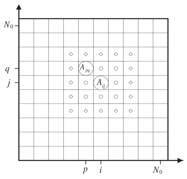
Figure 1:

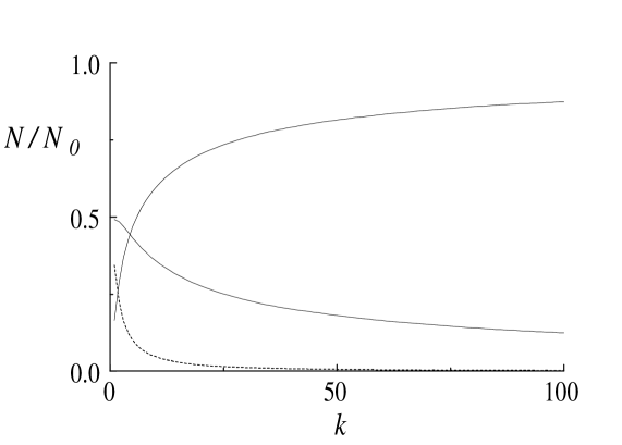
Figure 2:

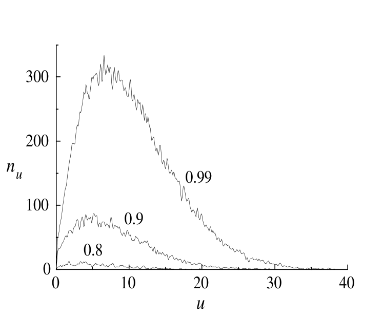
Figure 3:

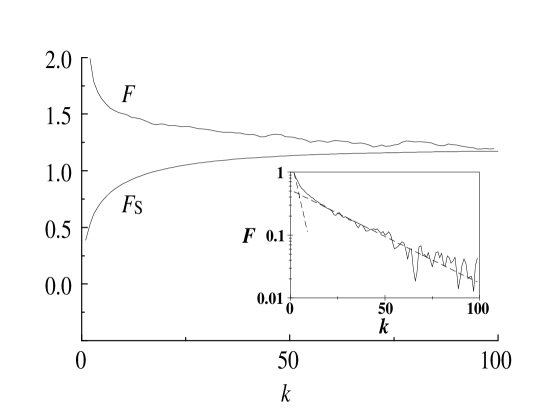
Figure 4:

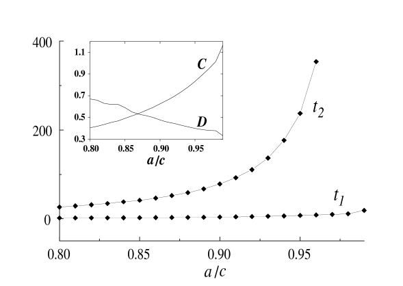
Figure 5:

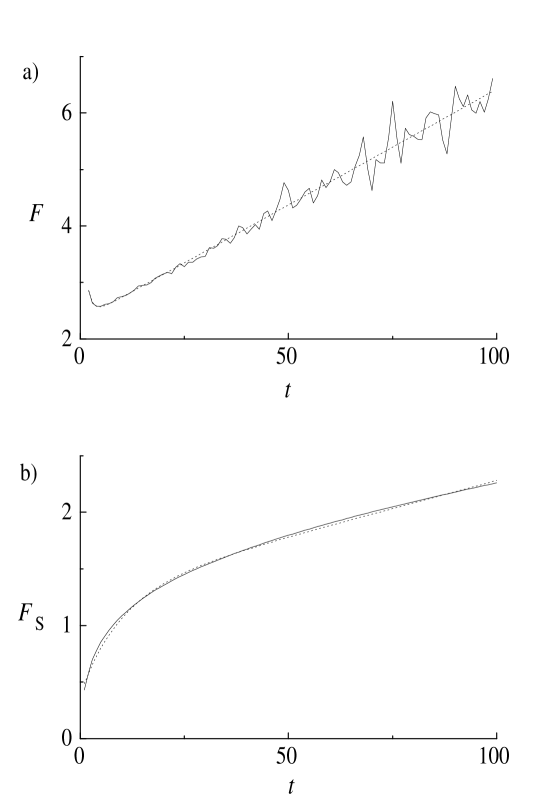
Figure 6:

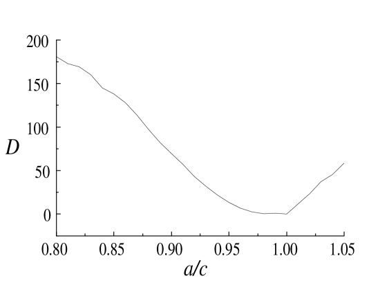
Figure 7: