Transitions to the Fulde-Ferrell-Larkin-Ovchinnikov phases at low temperature in two dimensions

Abstract

We explore the nature of the transition to the Fulde-Ferrell-Larkin- Ovchinnikov superfluid phases in the low temperature range in two dimensions, for the simplest isotropic BCS model. This is done by applying the Larkin-Ovchinnikov approach to this second order transition. We show that there is a succession of transitions toward ever more complex order parameters when the temperature goes to zero. This gives rise to a cascade with, in principle, an infinite number of transitions. Except for one case, the order parameter at the transition is a real superposition of cosines with equal weights. The directions of these wavevectors are equally spaced angularly, with a spacing which goes to zero when the temperature goes to zero. This singular behaviour in this $T=0$ limit is deeply linked to the two-dimensional nature of the problem.

PACS numbers : 74.20.Fg, 74.60.Ec

I INTRODUCTION

The possible existence of the Fulde-Ferrell-Larkin-Ovchinnikov (FFLO) superfluid phases [1, 2] has been pointed out in the early sixties and it has given rise to much work ever since that time. In addition to their intrinsic fundamental interest [3], these phases are quite relevant experimentally since they are expected to arise in superconductors with very high critical fields, which are naturally very actively searched for. On several occasions these phases have been claimed to be observed experimentally, but to date these hopes have not been firmly substantiated. Very recently anomalies in the heavy fermion compound CeCoIn₅ have been attributed to FFLO phases [4]. The case of two-dimensional (2D) systems is of particular interest [5] since they are experimentally quite relevant. Indeed a major strategy to observe these transitions is to eliminate orbital currents, which are responsible for the low critical fields in standard superconductors. This can be achieved in quasi two- dimensional systems, made of widely separated conducting planes, such as organic compounds or high $T_{c}$ cuprate superconductors. In this case hopping between planes is very severely restricted. Hence the orbital currents perpendicular to the planes are very weak when a strong magnetic field is applied parallel to the planes, and there is essentially no orbital pair breaking effect which opens the path to FFLO phases at much higher fields. Indeed experimental results in organic compounds have been claimed quite recently [6, 7] to be compatible with the existence of FFLO phases. Naturally when the magnetic field is not exactly parallel to the planes, one finds in addition vortex-like structures and the physical situation gets even more complex [8].

The FFLO transition in 2D systems is believed to be second order and in particular Burkhardt and Rainer [9] have studied in details the transition to a planar phase, where the order parameter $\Delta({\bf r})$ is a simple $\cos({\bf q}.{\bf r})$ at the transition. This phase has been found by Larkin and Ovchinnikov [2] to be the best one in 3D at $T=0$ for a second order phase transition. And in 3D it is also found to be the preferred one in the vicinity of the tricritical point and below [10, 11, 12], although in this case the transition turns out to be first order (except at very low temperature). However it is not clear that this is always the case since, as first explored by Larkin and Ovchinnikov, this order parameter is in competition with any superposition of plane waves, provided that their wavevectors have all the same modulus. Indeed we have shown very recently [13] that, at low temperature, the transition is rather a first order one, toward an order parameter with a more complex structure. For example at $T=0$ it is very near the linear combination of three cosines oscillating in orthogonal directions.

In this paper we explore the low temperature range in 2D and show that the second order transition is indeed toward rather more complex order parameters. A short report of our results has already been published [14]. A first step in this direction is found in the recent work of Shimahara [15] who found a transition toward a superposition of three cosines. Here we show that, when the temperature is lowered toward $T=0$, one obtains a cascade of transitions toward order parameters with an ever increasing number of plane waves. The $T=0$ limit is singular in this respect. This is actually clear from the beginning. Indeed if one looks at the second order term in the expansion of the free energy in powers of the order parameter, which gives the location of the FFLO transition, one finds it to be a singular function of the plane wave wavevector. This is recalled in the next section. Then we calculate the fourth order term in the free energy expansion and show that the phases which are selected by this term display the cascade of transitions mentionned above.

II THE FREE ENERGY EXPANSION : SECOND ORDER TERM

The general expression for the free energy difference $\Omega\equiv\Omega_{s}-\Omega_{n}$ between the superconducting and the normal state can be obtained in a number of ways, starting for example [9, 16, 17] from Eilenberger’s expression in terms of the quasiclassical Green’s function or from the gap equation [2] and Gorkov’s equations. When the result is expanded up to fourth order term in powers of the Fourier components $\Delta_{{\bf q}}$ of the order parameter $\Delta({\bf r})$:

$$\Delta({\bf r})=\sum_{{\bf q}_{i}}\Delta_{{\bf q}_{i}}\exp(i{\bf q}_{i}.{\bf r})$$ (1)

one obtains:

$$\frac{\Omega}{N_{0}}=\sum_{{\bf q}}\Omega_{2}(q,\bar{\mu},T)|\Delta_{{\bf q}}|^{2}+\frac{1}{2}\sum_{{\bf q}_{i}}\Omega_{4}({{\bf q}}_{1},{{\bf q}}_{2},{{\bf q}}_{3},{{\bf q}}_{4},\bar{\mu},T)\Delta_{{\bf q}_{1}}\Delta^{*}_{{\bf q}_{2}}\Delta_{{\bf q}_{3}}\Delta^{*}_{{\bf q}_{4}}$$ (2)

where we have momentum conservation ${\bf q}_{1}+{\bf q}_{3}={\bf q}_{2}+{\bf q}_{4}$ in the fourth order term and $N_{0}$ is the single spin density of states at the Fermi surface. The explicit expression of $\Omega_{2}(q,\bar{\mu},T)$ in terms of the standard BCS interaction $V$ and of the free fermions propagator is:

$$N_{0}\Omega_{2}(q,\bar{\mu},T)=\frac{1}{V}-T\sum_{n,k}\bar{G}({\bf k})G({\bf k}+{\bf q})$$ (3)

where $G({\bf k})=(i\bar{\omega}_{n}-\xi_{{\bf k}})^{-1}$ and $\bar{G}({\bf k})=(-i\bar{\omega}_{n}-\xi_{{\bf k}})^{-1}$ and $\bar{\omega}_{n}\equiv\omega_{n}-i\bar{\mu}$, with $\bar{\mu}=(\mu_{\uparrow}-\mu_{\downarrow})/2$ being half the chemical potential difference between the two fermionic populations forming pairs, $\xi_{{\bf k}}$ the kinetic energy measured from the Fermi surface for $\bar{\mu}=0$ and $\omega_{n}=\pi T(2n+1)$ the Matsubara frequency. Performing the $\xi_{{\bf k}}$ integration and the 2D angular average over $\hat{\bf k}$ gives:

$$\Omega_{2}(q,\bar{\mu},T)=\frac{1}{N_{0}V}+2\pi T\>{\rm Im}\sum_{n=0}^{\omega_{c}}\frac{1}{\sqrt{(i\bar{\omega}_{n})^{2}-\bar{\mu}^{2}\bar{q}^{2}}}$$ (4)

where we have introduced the dimensionless wavevector $\bar{q}=qv_{F}/2\bar{\mu}$. In Eq.(4) the summation has to be cut-off at a frequency $\omega_{c}$ in the standard BCS way. It is more convenient to rewrite $\Omega_{2}$, by introducing physical quantities related to the $\bar{q}=0$ case, as:

$$\Omega_{2}(q,\bar{\mu},T)=a_{0}(\bar{\mu},T)+I(q,\bar{\mu},T)$$ (5)

with:

$$I(q,\bar{\mu},T)=2\pi T\>{\rm Im}\sum_{n=0}^{\infty}\frac{1}{\sqrt{(i\bar{\omega}_{n})^{2}-\bar{\mu}^{2}\bar{q}^{2}}}-\frac{1}{i\bar{\omega}_{n}}$$ (6)

We have introduced:

$$a_{0}(\bar{\mu},T)=\frac{1}{N_{0}V}-2\pi T\>{\rm Re}\sum_{n=0}^{\omega_{c}}\frac{1}{\bar{\omega}_{n}}$$ (7)

which is zero on the spinodal transition line (the line in the $\bar{\mu},T$ plane where the normal state becomes absolutely unstable against a transition toward a space independent order parameter) and is positive above it. At the FFLO transition we are looking at, we have $\Omega_{2}(q,\bar{\mu},T)=0$. The actual transition corresponds to the largest possible $\bar{\mu}$ at fixed $T$. From Eq.(7) this corresponds to have the largest $a_{0}(\bar{\mu},T)$. Hence from Eq.(5) we want to minimize $I(q,\bar{\mu},T)$ with respect to $q$. At low temperature it is more convenient to express $I$ as:

$$I(q,\bar{\mu},T)=-\frac{1}{2}\>{\rm Re}\int_{-\infty}^{\infty}\!d\omega\>\tanh(\frac{\omega}{2T})\,[\frac{1}{\sqrt{(\omega+\bar{\mu})^{2}-\bar{\mu}^{2}\bar{q}^{2}}}-\frac{1}{\omega+\bar{\mu}}]$$ (8)

where the integration contour runs actually infinitesimally above the real $\omega$ axis.

At $T=0$ the integration is easily performed to give:

$$I(q,\bar{\mu},T)={\rm Re}\ln(1+\sqrt{1-\bar{q}^{2}})-\ln 2$$ (9)

The minimum is reached for $\bar{q}=1$ , in agreement with Shimahara [5] and Burkhardt and Rainer [9], and $I=-\ln 2$ at this minimum. In this case, from Eq.(7), $a_{0}(\bar{\mu},0)=\ln(2\bar{\mu}/\Delta_{0})$ where $\Delta_{0}=2\omega_{c}\exp(-1/N_{0}V)$ is the zero temperature BCS phase gap (this corresponds to the value $\bar{\mu}=\Delta_{0}/2$ for the spinodal transition). This leads to $\bar{\mu}=\Delta_{0}$ for the location of the FFLO transition, again in agreement with previous work. It is worth to note that, as already mentionned in the introduction, the location $\bar{q}=1$ of the minimum corresponds to a singular point for $I$ since we have explicitely $I=\ln(\bar{q}/2)$ for $\bar{q}>1$. While $I$ itself is continuous, its derivative is discontinuous for $\bar{q}=1$.

For $T\neq 0$ there is no singular behaviour and we find the value of $\bar{q}$ giving the minimum $I$ by writing that its derivative with respect to $\bar{q}$ is zero. Integrating the result by parts leads to the condition:

$${\rm Re}\int_{-\infty}^{\infty}\!dy\>\frac{1}{\cosh^{2}y}\,\frac{1+2ty}{\sqrt{(1+2ty)^{2}-\bar{q}^{2}}}=2$$ (10)

where we have taken the new variable $y=\omega/2T$ and defined the reduced temperature $t=T/\bar{\mu}$. Only the ranges $y>(\bar{q}-1)/2t\equiv a$ and $y<-(\bar{q}+1)/2t$ contribute to the real part of the integral. Since at low $T$ we have $\bar{q}\approx 1$, this last range will only give an exponentially small contribution because of the factor $\cosh^{-2}y$. Since this same factor makes $|y|$ to be at most of order 3 , we can make at low $T$ to leading order $1+2ty\approx 1$ and $(1+2ty)^{2}-\bar{q}^{2}\approx 2(1-\bar{q}+2ty)$. It is then seen that we must have $(\bar{q}-1)/2t\gg 1$, because $(\bar{q}-1)/2t\approx 1$ makes the left hand side of Eq.(10) much larger than unity at low $T$. This implies $y\gg 1$ and $2\cosh y\approx\exp y$. The integral is then easily evaluated and Eq.(10) gives finally to leading order:

$$\bar{q}-1=\frac{t}{2}\,\ln\frac{\pi}{2t}$$ (11)

Note that this result is in disagreemeent with the analysis given [18] by L. N. Bulaevskii. The reason for this discrepancy is discussed in details in Appendix A. In particular we rederive in this appendix our Eq. (10) from the starting equation of Ref. [18].

A more complete low temperature expansion can be fairly easily extracted from Eq.(10). As previously seen, the range $y>a$ in the integration is sufficient since the other integration range gives an exponentially small term. With the change of variable $y=u^{2}+a$, Eq.(10) leads to:

$$\int_{0}^{+\infty}du\frac{1+2\bar{t}u^{2}}{\cosh^{2}(u^{2}+a)\sqrt{1+\bar{t}u^{2}}}=2\sqrt{\bar{t}}$$ (12)

where we have defined $\bar{t}=t/\bar{q}$. Neglecting terms of order $\bar{t}^{2}$ Eq. (12) can be written as:

$$\int_{0}^{+\infty}\frac{du}{\cosh^{2}(u^{2}+a)}+\frac{3}{2}\bar{t}\int_{0}^{+\infty}\frac{u^{2}du}{\cosh^{2}(u^{2}+a)}=2\sqrt{\bar{t}}$$ (13)

From Eq.(11) the leading order for $a$ is $a_{0}=(1/4)\ln(\pi/2\bar{t})\gg 1$. In the second integral in Eq.(13) we can replace $a$ by $a_{0}$ since $\exp(-2a_{0})=\sqrt{2\bar{t}/\pi}\ll 1$. Setting $a=a_{0}+\delta a$, we obtain an expansion of $\delta a$ in powers of $\bar{t}^{1/2}$ by expanding the first integral up to second order in powers of $\delta a$:

$$-\frac{4}{\sqrt{\pi}}\bar{t}+\frac{4\sqrt{3}}{\pi}\bar{t}^{3/2}+\delta a\left(-4\bar{t}^{1/2}+\frac{16}{\sqrt{\pi}}\bar{t}\right)+4(\delta a)^{2}\bar{t}^{1/2}+\frac{3}{4}\bar{t}^{3/2}=0$$ (14)

valid up to the order $\bar{t}^{3/2}$. Solving this equation order by order, we find the following expansion for $a$:

$$a=\frac{1}{4}\ln\left(\frac{\pi}{2\bar{t}}\right)-\sqrt{\frac{\bar{t}}{\pi}}+\bar{t}\left(\frac{3}{16}+\frac{\sqrt{3}}{\pi}-\frac{3}{\pi}\right)+{\cal O}(\bar{t}^{3/2}).$$ (15)

This expression leads to a marked improvement when it is compared to the straight numerical evaluation of the Matsubara sums in Eq.(6). This is seen in Fig.1 where we have plotted the optimal $a=(\bar{q}-1)/2t$ from straight numerical calculation, as well as its leading low temperature approximation and the one resulting from the expansion Eq.(15). We give also for convenience, in the lower panel, the dependence of our reduced temperature $\bar{t}$ as a function of the ratio $T/T_{c0}$, where $T_{c0}$ is the standard BCS critical temperature, found for $\bar{\mu}=0$. In the low temperature limit $T\rightarrow 0$, we have merely $\bar{q}=1$ and $\bar{\mu}=\Delta_{0}$, hence $\bar{t}=T/\Delta_{0}$ and the dotted straight line in the lower panel gives this limiting behaviour $T/T_{c0}=\bar{t}\Delta_{0}/T_{c0}$.

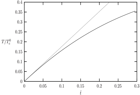
FIG. 1.: $a=(\bar{q}-1)/2t$ from the leading low temperature approximation Eq.(11) (dashed-dotted line), the low temperature expansion Eq. (15) (dotted line) and the full numerical calculation (full line), as a function of $\bar{t}=t/\bar{q}$. The lower panel gives the relation between $\bar{t}$ and $T/T_{c0}$ (full line), the dotted line is the low temperature limiting behaviour $T/T_{c0}=\bar{t}\Delta_{0}/T_{c0}=1.76\bar{t}$.

III FOURTH ORDER TERM

A Leading behaviour

The second order term in the free energy gives the same transition line for all the combinations of plane waves. The selection among the various possible order parameters will be made by the fourth order term in the free energy expansion, as pointed out by Larkin and Ovchinnikov. The selected state will correspond to the lowest fourth order term. So we turn now to this fourth order term. Its general expression is given by Eq.(2) with [2] :

$$N_{0}\Omega_{4}({{\bf q}}_{1},{{\bf q}}_{2},{{\bf q}}_{3},{{\bf q}}_{4},\bar{\mu},T)=T\sum_{n,k}\bar{G}({\bf k})G({\bf k}+{\bf q}_{1})\bar{G}({\bf k}+{\bf q}_{1}-{\bf q}_{4})G({\bf k}+{\bf q}_{2})$$ (16)

where we have used already momentum conservation ${\bf q}_{1}+{\bf q}_{3}={\bf q}_{2}+{\bf q}_{4}$. Since all the wavevectors ${\bf q}_{i}$ have the same modulus given by Eq.(11), this momentum conservation implies in our 2D situation either [2] ${\bf q}_{1}={\bf q}_{2}$ together with ${\bf q}_{3}={\bf q}_{4}$, or equivalently ${\bf q}_{1}={\bf q}_{4}$ together with ${\bf q}_{3}={\bf q}_{2}$. Moreover one has the additional possibility ${\bf q}_{1}=-{\bf q}_{3}$ together with ${\bf q}_{2}=-{\bf q}_{4}$. The two first possibilities lead to a same coefficient called $J(\alpha_{{\bf q}_{1},{\bf q}_{3}})$ by LO where $\alpha_{{\bf q}_{1},{\bf q}_{3}}$ is the angle between ${\bf q}_{1}$ and ${\bf q}_{3}$. Similarly the last possibility leads to a coefficient $\tilde{J}(\alpha_{{\bf q}_{1},{\bf q}_{2}})$. Explicitely the fourth order term in the free energy (last term of the r.h.s. of Eq.(2)) becomes [2] :

$$\frac{1}{2}\sum_{i,j}(2-\delta_{{\bf q}_{i},{\bf q}_{j}})|\Delta_{{\bf q}_{i}}|^{2}|\Delta_{{\bf q}_{j}}|^{2}J(\alpha_{{\bf q}_{i},{\bf q}_{j}})+(1-\delta_{{\bf q}_{i},{\bf q}_{j}}-\delta_{{\bf q}_{i},-{\bf q}_{j}})\Delta_{{\bf q}_{i}}\Delta_{-{\bf q}_{i}}\Delta^{*}_{{\bf q}_{j}}\Delta^{*}_{-{\bf q}_{j}}\tilde{J}(\alpha_{{\bf q}_{i},{\bf q}_{j}})$$ (17)

with, after a change of variable in the summation:

$$N_{0}J(\alpha_{{\bf q}_{1},{\bf q}_{2}})=T\sum_{n,k}\bar{G}({\bf k}+{\bf q}_{1})\bar{G}({\bf k}+{\bf q}_{2})G^{2}({\bf k})$$ (18)

and

$$N_{0}\tilde{J}(\alpha_{{\bf q}_{1},{\bf q}_{2}})=T\sum_{n,k}\bar{G}({\bf k})\bar{G}({\bf k}+{\bf q}_{1}+{\bf q}_{2})G({\bf k}+{\bf q}_{1})G({\bf k}+{\bf q}_{2})$$ (19)

When the $\xi_{{\bf k}}$ integration is performed, taking into account $\xi_{{\bf k}+{\bf q}}\approx\xi_{{\bf k}}+{\bf k}.{\bf q}/m$ since $q\ll k_{F}$, one finds:

$$J(\alpha_{{\bf q}_{1},{\bf q}_{2}})=4\pi T\>{\rm Im}\sum_{n=0}^{\infty}<\frac{1}{(2i\bar{\omega}_{n}+{\bf k}.{\bf q}_{1}/m)^{2}(2i\bar{\omega}_{n}+{\bf k}.{\bf q}_{2}/m)}+1\leftrightarrow 2>$$ (20)

where the bracket means the angular average, and similarly:

$$\tilde{J}(\alpha_{{\bf q}_{1},{\bf q}_{2}})=-16\pi T\>{\rm Im}\sum_{n=0}^{\infty}<\frac{i\bar{\omega}_{n}}{[(2i\bar{\omega}_{n})^{2}-({\bf k}.{\bf q}_{1}/m)^{2}].[(2i\bar{\omega}_{n})^{2}-({\bf k}.{\bf q}_{2}/m)^{2}]}>$$ (21)

on which it is clear that $\tilde{J}(\pi-\alpha)=\tilde{J}(\alpha)$.

Let us first consider $J(\alpha)$. As in the preceding section when going from Eq.(6) to Eq.(8), it is more convenient to transform the sum over Matsubara frequencies into an integral on the real frequency axis. When one furthermore performs a by parts integration over the frequency $\omega$, one gets from Eq.(20):

$$4\bar{\mu}^{2}J(\alpha)=-{\rm Re}\int_{-\infty}^{\infty}\!d\omega\>\frac{1}{\cosh^{2}(\omega/2T)}\int_{0}^{2\pi}\!\frac{d\theta}{2\pi}\frac{1}{[\bar{q}\cos(\theta-\alpha/2)-(1+\omega/\bar{\mu})].[\bar{q}\cos(\theta+\alpha/2)-(1+\omega/\bar{\mu})]}$$ (22)

where as above $\bar{q}=qk_{F}/2m\bar{\mu}$ and the integration contour runs again infinitesimally above the real $\omega$ axis. Here in the angular integration we have taken the reference axis bisecting the angle between ${\bf q}_{1}$ and ${\bf q}_{2}$. This angular integration is performed by residues, taking $\exp(i\theta)$ as a variable. For $Y=(1+\omega/\bar{\mu})/\bar{q}$ this leads to:

$$\int_{0}^{2\pi}\!\frac{d\theta}{2\pi}\frac{1}{[\cos(\theta-\alpha/2)-Y].[\cos(\theta+\alpha/2)-Y]}=\frac{Y}{(Y^{2}-\cos^{2}(\alpha/2))\sqrt{Y^{2}-1}}$$ (23)

where the cut in the determination of the square root has to be taken on the positive real axis, as it is clear when one considers the case of very large $|Y|$. When this result is inserted in Eq.(22) and $Y$ is taken as new variable, one finds, introducing again the reduced temperature $t=T/\bar{\mu}$:

$$16t\bar{\mu}^{2}\bar{q}J(\alpha)=-{\rm Re}\int_{-\infty}^{\infty}\!dY\>\frac{1}{\cosh^{2}((\bar{q}Y-1)/2t)}\frac{Y}{(Y^{2}-Y_{1}^{2})\sqrt{Y^{2}-1}}$$ (24)

with $Y_{1}=\cos(\alpha/2)$.

Up to now we have made no approximation in our calculation and the result is valid at any temperature. Let us now focus on the low temperature regime $t\ll 1$. Because of the factor $\cosh^{-2}((\bar{q}Y-1)/2t)$, only the vicinity of $Y=1$ will contribute. Moreover only the half circle contour around the pole $Y=Y_{1}$ and the range $Y>1$ contribute to the real part. In this last domain we have $(\bar{q}Y-1)/2t>(\bar{q}-1)/2t\gg 1$ from our result for $\bar{q}$ Eq.(11), so we can again simplify the hyperbolic cosine into an exponential (although this is not in practice a good approximation numerically). With the further change of variable $Y=1+tv^{2}/\bar{q}$ in the resulting integral, we find to leading order:

$$16t\bar{\mu}^{2}J(\alpha)=\frac{\pi}{\alpha}\frac{1}{\cosh^{2}[(1/4)\ln\frac{\pi}{2t}-\beta^{2}/2]}-\frac{8}{\sqrt{\pi}(1+\cos(\alpha/2))}\int_{0}^{\infty}\!dv\>\frac{\exp(-v^{2})}{v^{2}+\beta^{2}}$$ (25)

where we have substituted explicitely the result Eq.(11) for $\bar{q}$ and have set $\beta^{2}=(1-\cos(\alpha/2))/t$. The integral in this result can not be further simplified in general and is related to parabolic cylinder functions. Let us consider now some important limiting cases for this result. First we take at fixed $\alpha$ the limit $T\rightarrow 0$. This implies $\beta^{2}\rightarrow\infty$, the first term goes to zero and the integral is easily calculated in this limit, leading to:

$$J(\alpha)=-\frac{1}{4\mu^{2}}\frac{1}{\sin^{2}(\alpha/2)}$$ (26)

On the other hand if at fixed $T$ we take the limit $\alpha\rightarrow 0$, we have $\beta^{2}\rightarrow 0$. The limiting behaviour of the integral is $\pi/(2\beta)-\pi^{1/2}$ as can be obtained through a by parts integration, the dominant divergent contribution from the two terms cancels out and we are left with [19]:

$$J(\alpha)=\frac{1}{4\mu^{2}}\frac{1}{t}$$ (27)

which goes naturally to infinity for $T\rightarrow 0$. These two limits can be obtained more rapidly by making the proper simplifications from the start of the calculation Eq.(22).

The two limiting cases which we have just considered show that, at low temperature, $J(\alpha)$ has a quite remarkable behaviour. For most of the range it is negative as it can be seen from Eq.(26) and it even goes to large negative values when $\alpha$ gets very small. This tends to favor states with small angle between wavevectors, as we will see below. On the other hand for $\alpha=0$ or very small $J(\alpha)$ is positive and very large, as it results from Eq.(27). Clearly at low $T$ the interesting range is the small $\alpha$ domain where we can write $\beta=\alpha/(8t)^{1/2}$. Surprisingly $J(\alpha)$ first starts to increase strongly from its $\alpha=0$ value before going down to very negative values. This can be seen simply by looking at the specific point $\beta^{2}=(1/2)\ln(\pi/2t)$ for which the second term is negligible and which gives to dominant order $J(\alpha)=\pi/(32\mu^{2})t^{-3/2}(\ln(\pi/2t))^{-1/2}$, even more diverging for $T\rightarrow 0$ than the $T=0$ value. The integral of $J(\alpha)$ over $\alpha$ can also be analytically evaluated, and it shows that the strong positive peak at small $\alpha$ dominates over the negative contribution from the rest of the range. This quasi-singular behaviour of $J(\alpha)$ is summarized in Fig.2 where we have plotted $J(\alpha)$ for various temperatures.

We perform now the same kind of treatment for $\tilde{J}(\alpha)$. One goes again from Eq.(21) to an integration on the real frequency axis. However there is no integration by parts, and the angular average to be calculated is somewhat more complicated. It can nevertheless be performed by the same method and gives explicitely, with the same variable $Y=(1+\omega/\bar{\mu})/\bar{q}$ as above:

$$\int_{0}^{2\pi}\!\frac{d\theta}{2\pi}\frac{1}{[\cos^{2}(\theta-\alpha/2)-Y^{2}].[\cos(\theta+\alpha/2)^{2}-Y^{2}]}=\frac{1}{2Y\sqrt{Y^{2}-1}}(\frac{1}{Y^{2}-\cos^{2}(\alpha/2)}+\frac{1}{Y^{2}-\sin^{2}(\alpha/2)})$$ (28)

The second term is obtained from the first one by the change $\alpha\rightarrow\pi-\alpha$. This leads to $\tilde{J}(\alpha)=\tilde{J}_{o}(\alpha)+\tilde{J}_{o}(\pi-\alpha)$ with:

$$8\bar{\mu}^{2}\bar{q}^{2}\tilde{J}_{o}(\alpha)=-{\rm Re}\int_{-\infty}^{\infty}\!dY\>\tanh((\bar{q}Y-1)/2t)\frac{1}{\sqrt{Y^{2}-1}}\frac{1}{Y^{2}-\cos^{2}(\alpha/2)}$$ (29)

Here we have contributions coming from half circles around the poles at $Y=\pm\cos(\alpha/2)=\pm Y_{1}$ and contributions from the two domains $Y>1$ and $Y<-1$. Neglecting terms which are exponentially small in the low temperature limit, we can replace the hyperbolic tangent by $-1$ in the $Y<-1$ domain and for the $Y=-Y_{1}$ pole. Gathering similar contributions this gives:

$$8\bar{\mu}^{2}\bar{q}^{2}\tilde{J}_{o}(\alpha)=\frac{\pi}{\sin\alpha}\tanh((\bar{q}Y_{1}-1)/2t)+\int_{1}^{\infty}\!dY\>\frac{1-\tanh((\bar{q}Y-1)/2t)}{(Y^{2}-\cos^{2}(\alpha/2))\sqrt{Y^{2}-1}}+\frac{2\alpha-\pi}{\sin\alpha}$$ (30)

where we have used the fact that, without the $\tanh((\bar{q}Y-1)/2t)$ term, the integral can be performed exactly to give $(\pi-\alpha)/\sin\alpha$. We have taken advantage of this to have the factor $1-\tanh((\bar{q}Y-1)/2t)$ which is going rapidly to zero for large $Y$. This will be of use when we consider below temperature corrections. The last term in Eq.(30) disappears in the combination $\tilde{J}_{o}(\alpha)+\tilde{J}_{o}(\pi-\alpha)$, so we omit it from now on.

Looking now for the dominant contribution at low temperature, we simplify the hyperbolic tangent in the range $Y>1$ since its argument $(\bar{q}Y-1)/2t$ is large and positive. So one finds expressions which are similar to the one encountered in the calculation of $J(\alpha)$. Moreover, because of the relation $\tilde{J}(\pi-\alpha)=\tilde{J}(\alpha)$, we can restrict ourselves to the case $\alpha\leq\pi/2$. In this case the expression obtained by the replacement $\alpha\rightarrow\pi-\alpha$ is very simple since the corresponding value of $\beta^{2}=(1-\cos(\alpha/2))/t$ is always very large at low T. This leads finally to:

$$8\bar{\mu}^{2}\tilde{J}(\alpha)=-\frac{2\pi}{\sin\alpha}(1-\frac{1}{1+(2t/\pi)^{1/2}\exp(\beta^{2})})+\frac{2}{\sqrt{\pi}}\int_{0}^{\infty}\!dv\>\frac{\exp(-v^{2})}{v^{2}+\beta^{2}}$$ (31)

where we have taken into account that the second term is only significant when $\alpha$ is small, so we have made $\alpha=0$ in its prefactor.

In the limit $T\rightarrow 0$ with fixed $\alpha$, we have $\beta^{2}\rightarrow\infty$ and one gets merely:

$$\tilde{J}(\alpha)=-\frac{\pi}{4\mu^{2}}\frac{1}{\sin\alpha}$$ (32)

Again if we take $\alpha\rightarrow 0$ at fixed $T$, $\beta^{2}\rightarrow 0$, the dominant divergent contribution cancels and we find:

$$\tilde{J}(\alpha)=-\frac{1}{4\mu^{2}}$$ (33)

These two limits can be obtained again more directly. From these cases we can guess that $\tilde{J}(\alpha)$ is always negative. This is seen on Fig. 3 where $\tilde{J}(\alpha)$ has been plotted. However, in the same way as $J(\alpha)$, it has also a singular behaviour at small $\alpha$. While for $\beta\approx\alpha/(8t)^{1/2}\gg 1$ it diverges as $-\pi/(4\mu^{2}\alpha)$, it goes to the finite value $-1/(4\mu^{2})$ for $\alpha=0$. We note that the divergent behaviour in $\alpha^{-1}$ is weaker than the one in $\alpha^{-2}$ found for $J(\alpha)$ . Similarly $J(0)\gg|\tilde{J}(0)|$ at low $T$. So $J(\alpha)$ will play the dominant role and $\tilde{J}(\alpha)$ will only give a subdominant contribution.

B Temperature corrections

The expressions Eq.(24) and Eq.(31) found above respectively for $J(\alpha)$ and $\tilde{J}(\alpha)$ are the leading terms at low temperature. While containing the dominant physical behaviour, we do not expect them to be so good quantitatively at intermediate temperature. It is actually possible to improve these analytical results markedly in this respect at the price of a slight complication by including the first two terms in an expansion in powers of $\bar{t}^{1/2}$. This is the similar to what we have done at the end of section II for the second order term, and we follow here the same procedure, together with the steps we have just taken above for the calculation of $J(\alpha)$ and $\tilde{J}(\alpha)$.

We first consider first $J(\alpha)$ and start from the exact Eq.(24). Since the contribution from the domain $Y<-1$ is again exponentially small in the low temperature regime, we keep only the half circle contour around $Y_{1}$ and the $Y>1$ domain. The integral appearing in Eq.(24) can be split in two terms by:

$$\frac{Y}{Y^{2}-Y_{1}^{2}}=\frac{1}{2}\left(\frac{1}{Y-Y_{1}}+\frac{1}{Y+Y_{1}}\right).$$ (34)

Therefore $J(\alpha)$ can be written as $J(\alpha)=J_{o}(\alpha)+J_{o}(2\pi-\alpha)$ and we concentrate on the calculation of $J_{o}$. With the same notations $a=(\bar{q}-1)/2t$, $\bar{t}=t/\bar{q}$ and the change of variable $(\bar{q}Y-1)/2t=a+u^{2}$, Eq.(24) leads to:

$$32\bar{t}\bar{\mu}^{2}\bar{q}^{2}J_{o}(\alpha)=-\bar{t}^{-1/2}\int_{0}^{\infty}\frac{du}{\cosh^{2}(u^{2}+a)}\frac{1}{(u^{2}+\bar{\beta}^{2}/2)\sqrt{1+\bar{t}u^{2}}}+\frac{\pi}{\sin(\alpha/2)\cosh^{2}(a-\bar{\beta}^{2}/2)}$$ (35)

where we have set $\bar{\beta}^{2}=(1-\cos(\alpha/2))/\bar{t}$. The first term in the r.h.s. of Eq.(35) is expanded for low $t$ by $(1+\bar{t}u^{2})^{-1/2}\simeq 1-\bar{t}u^{2}/2$ and the resulting temperature correction is calculated to lowest order, replacing $a$ by $a_{0}=\ln(\pi/2\bar{t})/4$. This gives our following final expression, which has to be used together with Eq.(16) for $a$ and $\bar{q}$:

$$32\bar{t}\bar{\mu}^{2}\bar{q}^{2}J_{o}(\alpha)=-\bar{t}^{-1/2}\int_{0}^{\infty}\frac{du}{\cosh^{2}(u^{2}+a)}\frac{1}{u^{2}+\bar{\beta}^{2}/2}+\frac{\pi}{\sin(\alpha/2)\cosh^{2}(a-\bar{\beta}^{2}/2)}+\frac{2\bar{t}}{\sqrt{\pi}}\int_{0}^{\infty}dv\frac{v^{2}\exp(-v^{2})}{v^{2}+\bar{\beta}^{2}}$$ (36)

The second term in the r.h.s of this equation is only relevant for angles that are close to zero. Otherwise, it gives an exponentially small contribution in the low temperature limit. In the expression obtained by the change $\alpha\to 2\pi-\alpha$, this term is exponentially small in any case and can be forgotten. The first and the third term can be calculated more explicitly for angles $\alpha$ which are not close to zero (this is in particular the case for $J_{o}(2\pi-\alpha)$), which implies $\bar{\beta}\to+\infty$. For the first term in particular we can make use of our results in section II for the temperature expansion where similar terms were found. This leads finally in this regime to:

$$16\bar{\mu}^{2}\bar{q}^{2}J_{o}(\alpha)=-\frac{2}{1-\cos(\alpha/2)}+\bar{t}\>\frac{2-\cos\alpha/2}{(1-\cos(\alpha/2))^{2}}$$ (37)

For various temperatures, we compare in Fig. 2 these low temperature expressions with the exact calculation of $J(\alpha)$, from the direct numerical summation in Eq.(20) over Matsubara frequencies (with $\bar{q}$ obtained by the numerical minimisation of $I(q,\bar{\mu},T)$ given by Eq.(6)). We see that, at this level of accuracy, they agree remarkably well up to rather high temperatures.

FIG. 2.: $J(\alpha)$ for various values of the reduced temperature $\bar{t}=T/(\bar{q}\bar{\mu})=0.01$, $0.05$ and $0.1$. The lines are calculated using our low temperature expressions for $J(\alpha)$ and $a$, Eqs.(36) and (15), while the points correspond to the exact result numerical summation over Matsubara frequencies. The dashed line is the asymptotic behaviour for $J(\alpha)$ in the $T\to 0$ limit Eq.(26). The dashed-dotted lines are the leading order low temperature result Eq.(25)

We turn now to a similar calculation for $\tilde{J}(\alpha)$ and take up from Eq.(30). We have already pointed out that, since we can restrict ourselves to $0<\alpha<\pi/2$, the replacement $\alpha\to\pi-\alpha$ gives a value of $\bar{\beta}^{2}=(1-\cos(\alpha/2))/\bar{t}$ which is always large at low temperature. Therefore, in this replacement, the integral in Eq.(30) can be calculated to lowest order in $\bar{t}$ and gives $2\bar{t}/\cos^{2}(\alpha/2)$. In the same way in the first term the hyperbolic tangent can be replaced by -1 in this substitution. With the same change of variable as for $J(\alpha)$, we have finally:

$$8\bar{\mu}^{2}\bar{q}^{2}\tilde{J}_{o}(\alpha)=-\frac{\pi}{\sin\alpha}(1-\tanh(a-\bar{\beta}^{2}/2))+\frac{2\bar{t}}{\cos^{2}(\alpha/2)}+\bar{t}^{-1/2}\int_{0}^{\infty}du\frac{1-\tanh(u^{2}+a)}{(1+\cos(\alpha/2)+2\bar{t}u^{2})(u^{2}+\bar{\beta}^{2}/2)\sqrt{1+\bar{t}u^{2}}}$$ (38)

As for the calculation of $J(\alpha)$, we can have a more explicit result by expanding the denominator in the integral to first order in powers of $\bar{t}$ and computing the resulting temperature correction to lowest order by replacing $a$ by $a_{0}$. But we will not write the cumbersome resulting formula.

Nevertheless, as done previously for $J(\alpha)$, we compare in Fig. 3 our low temperature expressions with the exact calculation of $\tilde{J}(\alpha)$, $\bar{q}$ and $\bar{\mu}$. The discrepancy appears only above $\bar{t}\simeq 0.05$ in the vinicity of $\alpha=\pi/2$ and is mainly due to the fact that it becomes inaccurate to consider that $\beta^{2}$ is large in calculating $\tilde{J}_{o}(\pi-\alpha)$, as we have done (see above Eq.(31)). However our low temperature expressions are already sufficient to describe the cascade.

FIG. 3.: $\tilde{J}(\alpha)$ plotted for various values of the reduced temperature $\bar{t}=T/(\bar{q}\bar{\mu})=0.01$, $0.05$ and $0.1$. The lines correspond to the low temperature expressions for $\tilde{J}(\alpha)$ and $a$, Eqs. (38) and (15). while the dots show the exact results from numerical summation over Matsubara frequencies. The dashed line is the asymptotic behaviour Eq.(32).

IV Cascade of order parameter structures

A Ingredients responsible for the cascade

The second order term in the expansion of the free energy $\Omega$ gives the location of the transition $\bar{\mu}(T)$ and the optimum wavevectors modulus $\bar{q}$ entering the order parameter $\Delta({\bf r})$ but it can not distinguish between different order parameter structures, because from Eq.(2) the Fourier components $\Delta_{q}$ of the order parameter $\Delta({\bf r})$ are decoupled in the second order term. The resulting degeneracy is lifted by the fourth order term when one goes slightly into the superfluid phase. This is the basis of the analysis of Larkin and Ovchinnikov [2] and of Shimahara [15]. So to speak, the wavevectors directions are independent at the level of the second order term while the fourth order one provides an effective interaction between these directions. Since the expression Eq.(17) for the fourth order term depends only on the angle $\alpha_{n,m}$ between the wavevectors ${\bf q}_{n}$ and ${\bf q}_{m}$ through $J(\alpha_{n,m})$ and $\tilde{J}(\alpha_{n,m})$, the wavevector interaction appears therefore simply as pair interactions depending only on the relative positions of the 2D wavevectors on the circle. We note however that $\tilde{J}(\alpha_{n,m})$ corresponds to an interaction between two pairs of opposite wavevectors $({\bf q},-{\bf q})$ whereas $J(\alpha_{n,m})$ gives an interaction between two single wavevectors.

We consider now the ingredients which lead to the prediction of a cascade of transitions between order parameters with increasing number of wavevectors when the temperature goes to zero. First, since $J(\alpha)$ takes very large positive values for $\alpha$ smaller than a critical angle $\alpha_{0}$, we can consider that the angle domain $0<\alpha<\alpha_{0}$ is forbidden in order to avoid a dramatic increase of the free energy $\Omega$. To be quite specific we define $\alpha_{0}$ by $J(\alpha_{0})=0$. However we could as well take the critical angle as $\alpha_{c}$ which gives the minimum of $J(\alpha)$, since $\alpha_{0}$ and $\alpha_{c}$ are anyway very close as it can be seen on Fig.2 (we will indeed consider also $\alpha_{c}$ in the following). On the other hand it is favorable to take $\alpha$ slightly above $\alpha_{0}$ since it is the region where $J(\alpha)$ takes its most negative values. We note that the behavior of $\tilde{J}(\alpha)$ is not as strong compared to $J(\alpha)$, so we neglect $\tilde{J}(\alpha)$ in a first approximation. Next we see that $J(0)$ diverges as $1/T$ at low temperature and it is necessarily present in the free energy Eq.(17) from the terms with ${\bf q}_{n}={\bf q}_{m}$. However their unfavorable effect on $\Omega$ is lowered in relative value if one increases the number $N$ of wavevectors, since we have $N$ terms in Eq.(17) containing $J(0)$ compared to a total number of $N^{2}$ terms. Since we want to minimize $\Omega$, this leads us to increase $N$ and hence to decrease the angle between wavevectors as much as possible. Since the angle between wavevectors is bounded from below by $\alpha_{0}$, we expect for symmetry reasons that the optimum structure to have regularly spaced wavevectors with an interval angle slightly above $\alpha_{0}$. The last ingredient to predict the cascade is the fact that $\alpha_{0}$ decreases with temperature. As a result, the number $N$ of plane waves in the optimum structure increases when the temperature goes to zero. This leads to a cascade of states where the $T=0$ limit is singular. In the next sections, we present our arguments in more details.

B Study of the cascade

We begin by considering only the contribution $\Omega_{a}$ to the free energy $\Omega$ from the $J(\alpha)$ terms. Even so the full problem of finding the order parameter structure minimizing the fourth order term is not a simple one. However it is natural to assume that the wavevectors of the $N$ plane waves have a regular angular separation with an angle $2\pi/N$ between neighbouring wavevectors, so that their angular position is given on the circle by $\alpha_{n}=2n\pi/N$. Otherwise we would have a minimum corresponding to a disordered situation for the angles, which sounds quite unlikely (note that we can not collapse an angle to zero since we work at fixed $N$; we will later on minimize with respect to $N$). Then it is easy to show that the weight $w_{n}=|\Delta_{{\bf q}_{n}}|^{2}$ of the various wavevectors are all equal. Indeed the fourth order term Eq.(17) is just a quadratic form in $w_{n}$ and minimizing it is formally identical, for example, to find the lowest energy for a single particle in a tight binding Hamiltonian on a ring, with hopping matrix element $J(\alpha_{n,m})$ between site $n$ and site $m$ (except for the on-site term which is $J(0)/2$). The eigenvectors are plane waves and the eigenvalues are $J(0)/2+\sum_{n=1}^{N-1}J(\alpha_{n})\cos(n\phi_{k})$ with $\phi_{k}=2k\pi/N$ and $k=0,1,..,N-1$. Since $J(\alpha_{n})<0$ for $n\neq 0$, the lowest eigenvalue corresponds to $k=0$ which means that the weight $w_{n}$ are all equal.

Conversely if we assume from the start that the all weights $w_{n}$ are equal, our problem of finding the best $\alpha_{n}$’s is the same as the one of finding the equilibrium position of atoms on a ring with repulsive short range interaction (because $J(\alpha)$ is large and positive for small $\alpha$) and attractive long range interaction (because $J(\alpha)$ is negative for larger $\alpha$). We expect the equilibrium to correspond to a crystalline structure with regularly spaced atoms. This takes into account that $J(\alpha)$ is a long range potential (clearly this regular spacing would not be the equilibrium if we had a strongly short range potential enforcing a specific distance between our atoms). Naturally in this argument we take $N$ large enough to fill up the ring with atoms. So we come to the conclusion that the minimum energy corresponds to equally spaced wavevectors.

Finally when we minimize the total free energy Eq.(2) with respect to the weight $w_{n}$ we find the general result:

$$\frac{\Omega}{N_{0}}=-\frac{\Omega_{2}(q,\bar{\mu},T)^{2}}{G_{2}(N)}$$ (39)

where we have, in the case $\Omega=\Omega_{a}$:

$$NG_{2}(N)=2J(0)+4\sum_{n=1}^{N-1}J(\alpha_{n})$$ (40)

We note that we still have a degeneracy of the lowest energy configuration with respect to the choice of the plane waves phases.

We now take also into account in the free energy the terms containing $\tilde{J}(\alpha_{n,m})$. These terms appear when there are pairs of opposite wavevectors $({\bf q},-{\bf q})$. With our assumption of regularly spaced wavevectors, this corresponds to even $N$ - in which case we have $N/2$ pairs - whereas for odd $N$, there are no $\tilde{J}(\alpha_{n,m})$ terms in the free energy. Note that $\tilde{J}(\alpha)$ is negative for any angle $\alpha$ so that it is favorable to take pairs of opposite wavevectors. This seems to be in favor of taking $N$ even and we will indeed see that as a result states with even $N$ will be selected.

For even $N$, the total free energy is:

$$\frac{\Omega}{N_{0}}=\frac{\Omega_{a}}{N_{0}}+2\sum_{n=0}^{N/2-1}\sum_{m=0}^{N/2-1}(1-\delta_{n,m})\Delta_{n}\Delta_{-n}\Delta_{m}^{*}\Delta_{-m}^{*}\tilde{J}(\alpha_{n-m})$$ (41)

where we have used $\tilde{J}(\pi-\alpha)=\tilde{J}(\alpha)$ and $\alpha_{n,m}=2(n-m)\pi/N=\alpha_{n-m}$; $\Delta_{n}$ is a shorthand for $\Delta_{{\bf q}_{n}}$ and so on. The fact that $\tilde{J}(\alpha)$ is always negative has a direct consequence on the phases of the plane waves. In order to minimize the free energy they have to be chosen so that $\Delta_{n}\Delta_{-n}\Delta_{m}^{*}\Delta_{-m}^{*}$ is always real. Writing $\Delta_{n}=|\Delta_{n}|e^{i\phi_{n}}$, this implies that $\phi_{n}+\phi_{-n}=\Phi_{0}$ for any $n$, where $\Phi_{0}$ is a constant phase which can be chosen to be zero, since this merely corresponds to a global phase change for the order parameter. This link between phases for opposite wavevectors removes only a part of the degeneracy, since the phase $\phi_{n}=-\phi_{-n}$ can be still arbitrarily chosen. Now we see that the contribution of the $\tilde{J}(\alpha_{n,m})$ terms to the free energy is a quadratic form in $w^{\prime}_{n}=\Delta_{n}\Delta_{-n}$ with negative coefficients, and no on-site contribution. This is quite similar to what we have found for the $J(\alpha)$ terms in the preceding subsection. So the equal weight distribution, which minimizes the $J(\alpha)$ terms, gives also independently the minimum of the contribution of the $\tilde{J}(\alpha)$ terms. This means that the inclusion of these last terms in the free energy does not change the optimum structure apart from the phase link between opposite wavevectors. Finally the total minimum free energy is still given by Eq.(39), where Eq.(40) is valid for odd $N$, but has to be replaced for even N by:

$$NG_{2}(N)=2J(0)+4\sum_{n=1}^{N-1}J(\alpha_{n})+4\sum_{n=1}^{N/2-1}\tilde{J}(\alpha_{n})$$ (42)

In this last case the corresponding equilibrium order parameter is real, being a sum of cosines of the form $\Delta({\bf r})=|\Delta_{1}|\sum_{i}\cos({\bf q}_{i}.{\bf r}+\Phi_{i})$. We turn now to the minimization of the free energy with respect to $N$.

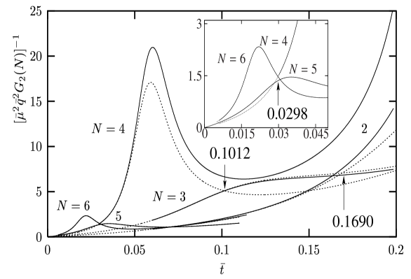
FIG. 4.: $[G_{2}]^{-1}$ as a function of the reduced temperature $\bar{t}=T/\bar{q}\bar{\mu}$, for different values of $N$. Full lines correspond to our analytical low temperature expressions from Eqs. (15), (36) and (38), while dashed lines show the exact result. They agree perfectly for $N=4,5,6$ in the $\bar{t}\leq 0.05$ domain.

C Minimization with respect to $N$.

We consider now the numerical calculation of $G_{2}(N)$ for different order parameter structures, i.e., for various values of the number of plane waves $N$. From Eq.(39) the equilibrium order parameter corresponds to the maximum $[G_{2}(N)]^{-1}$. In Fig. 4 we show for $[G_{2}(N)]^{-1}$ both our low temperature expansion and the exact evaluation of the Matsubara sum in Eqs. (20) and (21), as a function of the reduced temperature $\bar{t}$. We see that below $\bar{t}\simeq 0.05$, the low temperature analytical expressions, Eqs. (15), (36) and (38), agree remarkably well with the exact result. They are therefore completely sufficient quantitatively to study the cascade.

Fig. 5 displays the same quantity for lower temperatures, exhibiting the cascade of transitions. An interesting feature of this cascade is that an order parameter with an odd number of plane waves is never the lowest energy solution, except from the $N=3$ case, already found by Shimahara [15] . The reasons for this result will appear clearly in the next section, where we will study analytically the asymptotic regime of low temperatures.

V Low temperature asymptotic behaviour

A Minimum angle

In the low temperature limit $t\ll 1$, we can derive an explicit expansion for the value of the zero $\alpha_{0}$ of $J(\alpha)$, as well as the location $\alpha_{c}$ of its minimum. These critical angles are crucial to study the cascade since they give essentially the minimum angle between two wavevectors. In this low temperature range we have $\bar{q}\simeq 1$, so that $\bar{t}\simeq t$. As can be seen in Fig.2, $J(\alpha)$ has two extrema: a maximum for $\alpha$ around $a\simeq\beta^{2}/2$, as it is clear from the $\cosh^{-2}$ term in Eq.(25), and, for a slightly larger value of $\alpha$, a minimum at $\alpha_{c}$. The zero $\alpha_{0}$ is naturally in between. The condition $\beta^{2}/2\simeq a\simeq a_{0}=(1/4)\ln(\pi/2t)$ implies $\alpha\simeq 2\sqrt{t\ln(\pi/2t)}$. Therefore at low $t$, both $\alpha_{0}$ and $\alpha_{c}$ are in a domain where $\alpha\to 0$ and $x=\beta^{2}/2=\alpha^{2}/16t\to+\infty$. In this regime the two terms in Eq.(25) for $J(\alpha)$ simplify to give:

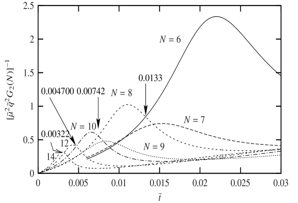
FIG. 5.: $G_{2}$ plotted for temperatures lower and values of $N$ higher than in Fig.4, using Eqs. (15), (36) and (38). For clarity we do not represent solutions of $N$ larger than $14$ but they can be easily numerically evaluated.

$$\bar{\mu}^{2}J(\alpha)\simeq\frac{\pi}{16t\alpha\cosh^{2}X}-\frac{1}{\alpha^{2}}$$ (43)

where $X=x-a_{0}$. The second term in this expression simply comes from $-1/4\sin^{2}(\alpha/2)$ which is the asymptotic limit Eq.(26) for $\bar{\mu}^{2}J(\alpha)$.

Let us first consider the calculation of $\alpha_{c}$. The first term is responsible for the strong upturn near the minimum. From the derivative of Eq.(43) $J(\alpha)$ is extremal for:

$$\cosh^{2}X=\frac{\pi}{2}\frac{x^{3/2}}{t^{1/2}}(\tanh X+\frac{4}{x})$$ (44)

The minimum we are looking for is in the domain $X>0$ and from the above equation it is found for a large value of $X$. This allows to simplify this equation into:

$$e^{x}=kx^{3/4}$$ (45)

with $k=(2\pi^{3}/t^{2})^{1/4}$. Writing this equation $x=\ln k+(3/4)\ln x$ one can generate a solution by the recurrence relation $x_{n+1}=\ln k+(3/4)\ln x_{n}$ which converges very rapidly. For example the second iteration gives:

$$x=\ln k+(3/4)\ln[\ln k+(3/4)\ln(\ln k)]$$ (46)

The corresponding result for $\alpha_{c}$ is to leading order in the low temperature limit:

$$\alpha_{c}=\left(8t\ln\frac{(2\pi^{3})^{1/2}}{t}\right)^{\frac{1}{2}}$$ (47)

but numerically this is not such a good result at low temperature and one has rather to perform a few iterations to get the correct answer. For example in Eq.(45), the exact result is $x=5.94$ for $k=100$, while $\ln k=4.60$, but the second iteration Eq. (46) gives $x=5.92$.

Then in order to find the optimum number of plane waves we notice that $J(\alpha)$ rises very rapidly below $\alpha_{c}$, so we can not have basically the angular separation $2\pi/N$ between two plane waves less than $\alpha_{c}$. Since on the other hand it is energetically favorable to take $N$ as large as possible, as long as $J(\alpha)$ is negative, we can find an asymptotic estimate of the optimum value $N_{o}$ of $N$ by taking the integer value of $2\pi/\alpha_{c}$, that is:

$$N_{o}={\rm E}\left[\frac{2\pi}{\alpha_{c}}\right]$$ (48)

Following the same procedure, we can also derive an explicit expression for the angle $\alpha_{0}$ corresponding to the zero of $J(\alpha)$. From Eq.(43), we find:

$$\cosh^{2}X=\frac{\pi\alpha}{16t}.$$ (49)

Naturally $\alpha_{0}$ is close to $\alpha_{c}$ since $J(\alpha)$ is rapidly increasing below $\alpha_{c}$. We are still in the $X>0$ domain and the solution corresponds to $X$ large. This simplifies the above equation into:

$$e^{x}=\frac{k}{\sqrt{2}}x^{1/4}$$ (50)

where $k$ has been defined previously. The corresponding recurrence relation which generates the exact solution is $x_{n+1}=\ln(k/\sqrt{2})+(1/4)\ln x_{n}$. The second iteration gives here:

$$x=\ln\frac{k}{\sqrt{2}}+\frac{1}{4}\ln\left[\ln\frac{k}{\sqrt{2}}+\frac{1}{4}\ln\left(\ln\frac{k}{\sqrt{2}}\right)\right]$$ (51)

and $\alpha_{0}$ is simply given by $\alpha_{0}=\sqrt{16tx}$. We can then make the same argument as above for $\alpha_{c}$, and write the following asymptotic estimate of the optimum value $N_{o}$:

$$N_{o}={\rm E}\left[\frac{2\pi}{\alpha_{0}}\right]$$ (52)

which will naturally be found to be quite near the above one Eq.(48), since $\alpha_{0}$ and $\alpha_{c}$ are quite close.

Naturally we can calculate numerically exactly the optimal value $N_{0}$ of $N$ as a function of the temperature, from our above results. In the same process we find also the critical temperatures where the $N_{0}$ changes. They are given by the crossings of the $G_{2}(N)$ curves for different values of $N$, as it is seen on Fig. 4 and 5. In Fig. 6 these exact critical temperatures are compared with the exact calculations of $2\pi/\alpha_{c}$ and $2\pi/\alpha_{0}$, as well as their asymptotic values. As it is seen on this figure, it happens that the optimal values of $N$ falls essentially just between $2\pi/\alpha_{c}$ and $2\pi/\alpha_{0}$ in the low temperature domain.

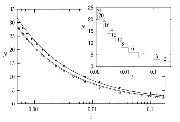
FIG. 6.: Optimal value of $N$ and locations of the critical temperatures. The dots give the temperatures where the optimal $N$ changes: the white dot is the optimal $N$ above the critical temperature whereas the black dot is the optimal $N$ below. $2\pi/\alpha_{c}$ (curves very near the white dots) and $2\pi/\alpha_{0}$ (curves very near the black dots) are also shown on this figure. The dashed lines show the exact calculations,while the solid lines are determined with the recurrence formulas below Eq. (45) and Eq. (50) with only one iteration. In the insert for clarity we only show the ”devil” staircase corresponding to the white and black dots.

B Asymptotic evaluation of $G_{2}(N)$

It can be seen on Fig. 2 that $J(\alpha)$ switches rapidly above $\alpha_{c}$ to its large angle asymptotic behaviour:

$$\bar{\mu}^{2}J(\alpha)\simeq-\frac{1}{4\sin^{2}(\alpha/2)}$$ (53)

so we may with a fair precision use this simplified expression for $J(\alpha_{n})$, with $\alpha_{n}=2\pi n/N$, to evaluate the sum in Eq.(40) for $G_{2}(N)$. At low temperature the number of plane waves N is large and the sum is dominated by the terms with small $n$ corresponding to small angles, for which we have $\sin(\alpha/2)\simeq\alpha/2$. Hence we have for the sum coming in Eq. (40) for $G_{2}(N)$:

$$\frac{4}{N}\sum_{n=1}^{N-1}\bar{\mu}^{2}J(\frac{2\pi n}{N})\simeq-\frac{8}{N}\sum_{n=1}^{N/2-1}\frac{1}{4(n\pi/N)^{2}}=-\frac{N}{3}+{\mathcal{O}}\left(\frac{1}{N}\right)$$ (54)

For even $N$, we have also to evaluate the contribution coming from the terms in Eq. (42) containing $\tilde{J}(\alpha)$. Again we can use for most angles the asymptotic expression Eq.(32) for $\tilde{J}(2\pi n/N)$. Once more the dominant contribution comes from the small $n$ terms, and the logarithmic leading behaviour is accurately given by the asymptotic expression of $\tilde{J}(\alpha)$ as:

$$\frac{4}{N}\sum_{n=1}^{N/2-1}\bar{\mu}^{2}\tilde{J}(\frac{2\pi n}{N})\simeq-\frac{2\pi}{N}\sum_{n=1}^{N/4}\frac{1}{2\pi n/N}=-\ln N+{\mathcal{O}}(1)$$ (55)

[VERIFIER le n=1]We see here explicitely that $J(\alpha)$ has a dominant role compared to $\tilde{J}(\alpha)$. Taking into account the $J(0)$ contributions, the dominant behaviour of $G_{2}(N)$ can be summarized in the limit of large plane wave number $N$ and low temperature as:

$$\bar{\mu}^{2}G_{2}(N) \simeq \frac{1}{2Nt}-\frac{N}{3}\qquad\qquad\qquad\qquad\qquad\qquad N\textrm{odd}$$ (56)

$$\bar{\mu}^{2}G_{2}(N) \simeq \frac{1}{2Nt}-\frac{N}{3}-\ln N+cte\qquad\qquad\qquad N\textrm{even}$$ (57)

These expressions correspond actually in Fig. 5 only to the rising part of $[G_{2}(N)]^{-1}$ on the low temperature side. The downturn of $[G_{2}(N)]^{-1}$ for higher temperature is due to contributions from the positive part of $J(\alpha)$ which are beyond our asymptotic approximation Eq. (53). Nevertheless we have also found above the critical temperatures for switching from a given value of $N$ to the next one. From Fig. 5 it is seen that it is enough to plug these critical temperatures into the evaluation of the rising part of $[G_{2}(N)]^{-1}$ to obtain the free energy at the transitions. When we substitute accordingly in these expressions Eq. (56) or (57) the value $N=2\pi/\alpha_{c}$ for the optimum plane wave number we have:

$$\bar{\mu}^{2}G_{2}(N)=\frac{\alpha_{c}}{4\pi t}\left(1-\frac{8\pi^{2}t}{3\alpha_{c}^{2}}\right)+{\mathcal{O}}(\ln(1/t))$$ (58)

Since $8t/\alpha_{c}^{2}\sim 1/\ln(1/t)$ from Eq.(47), we find that $G_{2}(N)$ is always positive in the low temperature range (more precisely we have $1-(8\pi^{2}t)/(3\alpha_{c}^{2})=1-\pi^{2}/6x$ which is positive as soon as $x>\pi^{2}/6$, i.e. from Eq.(45) exactly for $t<0.62$). This means that the transition stays always second order (a negative sign would have implied a first order transition and a breakdown of our fourth order expansion).

Finally it seems from Eq.(56-57) that it is favourable to have an even number of plane waves in order to take advantage of the additional $\tilde{J}$ contribution. This can be confirmed by a more careful comparison between two consecutives values of $N$. Let us assume that $N$ is odd with $N=2\pi/\alpha_{c}$ and compare $G_{2}(N)$ to $G_{2}(N-1)$. By going from $N$ to $N-1$ we gain naturally the $\tilde{J}$ term in Eq.(57), but we increase the first term due to the unfavorable of the $J(0)$ term. Nevertheless:

$$\bar{\mu}^{2}[G_{2}(N-1)-G_{2}(N)]=\frac{1}{2N(N-1)t}-\ln(N-1)+{\mathcal{O}}(1).$$ (59)

where the dominant term becomes exactly with the help of Eq.(45):

$$\bar{\mu}^{2}[G_{2}(N-1)-G_{2}(N)]=-x(1-\frac{2}{\pi^{2}})+\frac{5}{4}\ln x+\frac{1}{4}\ln\frac{32}{\pi}$$ (60)

which is always negative since its maximum, reached for $1/x_{m}=(4/5)(1-2/\pi^{2})$, is -0.107. Therefore the asymptotic evaluation of $G_{2}(N)$ shows indeed explicitely that the only order parameters which appears at low temperature are those with an even number of plane waves, in agreement with our exact numerical results.

C Phenomenological interpretation

It is interesting to compare our results to the pairing ring picture explored by Bowers and Rajagopal [20] (BR) in the three dimensional case. BR have looked at the free energy expansion at zero temperature in $3$D, extending the work of Larkin and Ovchinnikov. In the case of multiple plane waves in the order parameter, they have pointed out a simple physical interpretation of their results. Their picture is based on the Fulde and Ferrell study [1] of a single plane wave order parameter where they showed that one may separate the wavevector space in two complementary domains: the pairing region and the pair breaking region. In the case of a vanishing order parameter and considering only wavevectors at the Fermi surface, the pairing region is merely an infinitely thin circle. It is given by the intersection of the up and down spin Fermi surfaces, after shifting one of them by ${\bf q}$. The total opening angle of this circle is thereforer given by $\psi_{0}=\arccos(1/\bar{q})$. In $3$D and at $T=0$, $\bar{q}=1.1997$ which gives $\psi_{0}=67.1^{\circ}$. For a non-zero order parameter amplitude $\Delta$, the circle broadens and becomes a ring whose width is given by $\Delta/\bar{\mu}$. Therefore, the pairing region for a single plane wave is a ring drawn on the Fermi surface, whose center is on the plane wave direction ${\bf q}$ (the restriction to the Fermi surface is justified by the fact that only wavevectors close to the Fermi surface are relevant for pairing).

In the case of multiple plane waves in the order parameter, BR showed that the intersection of pairing circles from different plane waves is energetically largely unfavored, the worst case being when two circles are exactly in contact. The maximisation of the pairing regions leads naturally to increase as much as possible the plane waves number $N$ with the constraint that they are no intersecting circles. This leads to nine circles on the Fermi surface. BR rather concluded that the least energy state was the one with eight plane waves for ’regularity’ reasons. In particular, this leads to a real order parameter. We see now that our cascade in $2$D is a direct consequence of these two heuristic principles : the no-intersecting circles rule and the maximisation of plane waves.

In $2$D, the circles are replaced by pairs of points separated by the angle $\psi_{0}$, and the no-intersecting rule becomes now a no-entanglement rule between different pairs. But this is just equivalent to our above finding from Fig. 2 that there is an effective short range repulsion between different wavevectors ${\bf q}$, with indeed the worst case corresponding to the contact since the maximum of $J(\alpha)$ is just below its zero. The contact condition $a=\bar{\beta}^{2}/2$ that we have found (corresponding to the maximum of $J(\alpha)$) can be rewritten as $\cos(\alpha/2)=1/\bar{q}$ which implies $\alpha/2=\psi_{0}/2$. This is exactly the same as the contact condition of BR. Next we have found explicitely that it is indeed favorable to maximize the number of plane waves, taking the short range repulsion into account. Our cascade is due to the fact that, when the temperature goes to zero, $\psi_{0}$ also drops to zero and the pairing region for a single plane wave shrinks to a single point, corresponding to the situation where the two up and down Fermi circles are just in contact.

VI CONCLUSION

In this paper we have investigated the low temperature range for the FFLO transition in two dimensions and we have shown that the order parameter is no longer a simple $\cos({\bf q}.{\bf r})$ at the second order transition, in contrast with the situation found near the tricritical point. Instead the transition is toward more and more complex order parameters when the temperature goes to zero, which gives rise to a cascade with, in principle, an infinite number of transitions. At the transition these order parameters are in general a superposition of an even number of plane waves with equal weight and equal wavevector modulus, which corresponds to a real order parameter equal to a superposition of cosines. The directions of these wavevectors are found to be equally spaced angularly, with a spacing which goes to zero when the temperature goes to zero, which is the reason for the ever increasing number of plane waves in this limit. The singular behaviour in this limit $T=0$ is actually present in all physical quantities. It arises because, in order to obtain the lowest energy, the two Fermi circles corresponding to opposite spins come just in contact when one applies the shift corresponding to the wavevector ${\bf q}$ of the FFLO phase. This is this situation, with these two circles just touching each other, which gives rise to the singularities. Naturally this is linked to the fact that in 2D the Fermi surface is actually a line. Hence this singularity is a general feature of 2D physics and we may expect it to give rise to similar consequences in more realistic and more complex models describing actual physical systems.

Naturally in this paper we have addressed this remarkable situation in the most simple physical frame. We have considered the simplest BCS model with isotropic Fermi surface, that is a circle for our 2D case. Naturally if anisotropy is introduced in the dispersion relation of the electrons, or in the effective electron-electron interaction, or both, the physics will be more complex. In the same way we expect Fermi liquid effects [9] to bring important quantitative modifications. Similarly if we consider a quasi 2D superconductor with a magnetic field not perfectly aligned with the planes, currents will be produced and orbital contributions to the free energy will arise. However in order to have the physics right in all these complex situations, it is quite clear that one has to obtain the correct limit in the simplest possible case that we have considered in the present paper.

VII Appendix A

In this section we rederive rapidly our result Eq.(11) for the leading order of the optimal wavevector at low temperature, taking the same starting point as Bulaevskii [18].

We start from Eq.11 of Ref.[18]:

$$\ln(T_{c}/T)=\frac{1}{\pi}{\rm Re}\int_{-Pv_{F}}^{Pv_{F}}d\Omega\frac{1}{\sqrt{P^{2}v_{F}^{2}-\Omega^{2}}}[\psi(1/2+i(2\mu_{0}H+\Omega)/4\pi T))-\psi(1/2)]$$ (61)

We go to our notations by setting $H=\bar{\mu},P=q$ and introduce as above our reduced variables $\bar{q}=qv_{F}/2\bar{\mu}$ and $t=T/\bar{\mu}$. When we perform the angular integration as in Ref. [18] by setting $\Omega=Pv_{F}\cos\theta$ and introduce for the digamma function the integral representation (Eq.13 of Ref. [18]):

$$\psi(x)=\ln x-1/2x-2\int_{0}^{\infty}\frac{ydy}{(y^{2}+x^{2})(\exp(2\pi y)-1)}$$ (62)

we obtain Eq.14 of Ref. [18] (correcting some minor misprints). We can then expand the result to all orders in $t$ and show that all the terms in the expansion are zero. However rather than displaying the steps of this calculation here, it is more convenient to immediately remark that the optimal $\bar{q}$ is obtained by writing that the derivative of Eq.11 with respect to $\bar{q}$ is zero. This provides an equivalent calculation (we work on the derivative instead of working on the function), which is somewhat easier and allows us also to make in the following the direct contact with our result. This condition on the derivative, which gives the equation for the optimal $\bar{q}$, is:

$${\rm Im}\int_{0}^{\pi}\frac{d\theta}{\pi}\psi^{\prime}(1/2+i(1+\bar{q}\cos\theta)/2\pi t))=0$$ (63)

Taking the derivative of the above integral representation, we obtain a corresponding representation for $\psi^{\prime}$ on which the angular integration is easily performed (the integrals can be found in Gradstein and Ryzhik [21]). We display the result by introducing the function $f(x)=x/\sqrt{(}x^{2}-1)$ and setting $x_{0}=1/\bar{q}$ , $\epsilon=-i\pi t/\bar{q}$ and $x=x_{0}+\epsilon$. The result is:

$${\rm Re}\,[1-f(x)+\epsilon f^{\prime}(x)-\frac{\pi}{2}\int_{-\infty}^{\infty}\frac{dy}{\sinh^{2}(\pi y)}(f(x)-f(x_{0}+\epsilon(1+2iy)))]=0$$ (64)

where the integral goes from $-\infty$ to $\infty$ because we have collected two terms into one. Now we can write for the first three terms the Taylor expansion:

$$1-f(x)+\epsilon f^{\prime}(x)=1-f(x_{0})+\sum_{0}^{\infty}\frac{\epsilon^{n+1}}{n!}\frac{n}{n+1}f^{(n+1)}(x_{0})$$ (65)

When we take the real part, only the odd order derivatives of $f$ contribute because $\bar{q}$ is near $1$ with $\bar{q}>1$, which makes $x_{0}<1$ and $Ref^{(2p)}(x_{0})=0$. This gives:

$${\rm Re}\,[1-f(x)+\epsilon f^{\prime}(x)]=1+\sum_{p=1}^{\infty}\frac{\epsilon^{2p+1}}{(2p)!}\frac{2p}{2p+1}f^{(2p+1)}(x_{0})$$ (66)

Similarly we can perform the expansion in the integral and expand $(1+2iy)^{n}$ by introducing the binomial coefficients $C_{n}^{p}$. All the resulting integrals can be found in Gradstein and Ryzhik [21], and expressed in terms of Bernoulli numbers $B_{2m}$. This leads to:

$$\frac{\pi}{2}{\rm Re}\,\int_{-\infty}^{\infty}\frac{dy}{\sinh^{2}(\pi y)}[f(x)-f(x_{0}+\epsilon(1+2iy))]=\sum_{p=1}^{\infty}\frac{\epsilon^{2p+1}}{(2p+1)!}f^{(2p+1)}(x_{0})\sum_{m=1}^{p}C_{2p+1}^{2m}4^{m}B_{2m}$$ (67)

Now a remarkable identity (found for example in Gradstein and Ryzhik [21]) for Bernoulli numbers states that:

$$\sum_{m=1}^{p}C_{2p+1}^{2m}4^{m}B_{2m}=2p$$ (68)

As a result, by gathering all the terms, all the coefficients of the powers of $\epsilon$ are zero, and it is not possible to satisfy the condition that the above derivative is zero. The answer to this puzzle is that the contribution of the terms we have considered is not exactly zero, but exponentially small, which explains why we find it to be zero in a perturbative expansion. This is shown now in the following.

We start again from the above condition Eq.(64) found for the optimum wavevector. We transform the integral by shifting the integration contour toward the upper complex plane by $i/2$ for the variable $y$. First we have to take care that integrant in the above integral has no singularity for $y=0$, because proper cancellation between various terms. Hence we can also say that this integral is equal to its principal part. Next if we want a complete contour $C$, we have to add to this principal part the contribution of an infinitesimal semi-circle around $y=0$ with positive imaginary part. This contribution is easily found by residues to be equal to $-\epsilon f^{\prime}(x)$, so we have:

$${\rm Re}\,[\epsilon f^{\prime}(x)-\frac{\pi}{2}\int_{-\infty}^{\infty}\frac{dy}{\sinh^{2}(\pi y)}(f(x)-f(x_{0}+\epsilon(1+2iy)))]=-\frac{\pi}{2}{\rm Re}\,\int_{C}\frac{dy}{\sinh^{2}(\pi y)}[f(x)-f(x_{0}+\epsilon(1+2iy))]$$ (69)

Now we set $\pi y=z+i\pi/2$ and make use of $i\sinh(z+i\pi/2)=i\cosh(z)$ which gives:

$${\rm Re}\,[\epsilon f^{\prime}(x)-\frac{\pi}{2}\int_{-\infty}^{\infty}\frac{dy}{\sinh^{2}(\pi y)}(f(x)-f(x_{0}+\epsilon(1+2iy)))]=\frac{1}{2}{\rm Re}\,\int_{-\infty}^{\infty}\frac{dy}{\cosh^{2}z}(f(x)-f(x_{0}+2tz/\bar{q}))$$ (70)

where the contour runs infinitesimally below the real $z$ axis. The first term in the last integral is just equal to $f(x)$, so our equation becomes:

$${\rm Re}\,[1-\frac{1}{2}\int_{-\infty}^{\infty}\frac{dy}{\cosh^{2}(\pi y)}f(x_{0}+2tz/\bar{q})]=0$$ (71)

It is easily checked that this equation is identical to our Eq.(10). Note that the fact that the contour runs infinitesimally above or below the real axis is unimportant since we take the real part, and the contribution along the cut due to the square root is purely imaginary.

In conclusion we have obtained our basic equation for the second order term by taking the same starting point as Ref. [18]. The end of the argument to obtain Eq.(11) is naturally the same as following our Eq.(10). In particular this argument shows that the integral in the above formula is proportional to $\exp{[-(\bar{q}-1)/t]}$, so it can not be expanded in powers of $t$.

* Laboratoire associé au Centre National de la Recherche Scientifique et aux Universités Paris 6 et Paris 7.

REFERENCES

- [1] P. Fulde and R. A. Ferrell, Phys.Rev. 135, A550 (1964).
- [2] A. I. Larkin and Y. N. Ovchinnikov, ZhETF 47, 1136 (1964) [Sov. Phys. JETP 20, 762 (1965)].
- [3] See in particular R. Casalbuoni and G. Nardulli, Rev. Mod. Phys. 76, 263 (2004) for a review more particularly focused on the interest of the FFLO phases for quark matter, as might be found in neutron stars.
- [4] A. Bianchi, R. Movshovich, C. Capan, P. G. Pagliuso, and J. L. Sarrao, Phys. Rev. Lett. 91, 187004 (2003) and C. Martin, C. C. Agosta, S. W. Tozer, H. A. Radovan, E. C. Palm, T. P. Murphy, J. L. Sarrao, cond-mat/0309125, and references therein for other possible experimental observations.
- [5] H. Shimahara, Phys. Rev. B, 50, 12760 (1994).
- [6] J. Singleton, J. A. Symington, M. S. Nam, A. Ardavan, M. Kurmoo and P. Day, J. Phys. Cond. Mat. 12, L641 (2000).
- [7] M. A. Tanatar, T. Ishiguro, H. Tanaka and H. Kobayashi, Phys. Rev. B 66, 134503 (2002);
- [8] For recent papers on this question see for example U. Klein, Phys. Rev. B 69, 134518 (2004); M. Houzet and A. Buzdin, Europhys. Lett., 50, 375 (2000); K. Yang, A. H. MacDonald, cond-mat/0404580 and references therein.
- [9] H. Burkhardt and D. Rainer, Ann.Physik 3, 181 (1994).
- [10] S. Matsuo, S. Higashitani, Y. Nagato and K. Nagai, J. Phys. Soc. Japan, 67 280 (1998).
- [11] M. Houzet, Y. Meurdesoif, O. Coste and A. I. Buzdin, Physica C 316, 89 (1999).
- [12] R. Combescot and C. Mora, Eur.P.J. B 28, 397 (2002).
- [13] R. Combescot and C. Mora, cond-mat/0311042.
- [14] C. Mora and R. Combescot, to be published in Europhys. Lett.
- [15] H. Shimahara, J. Phys. Soc. Japan, 67, 736 (1998).
- [16] G. Eilenberger, Z. Phys. 182 427 (1965).
- [17] N. R. Werthamer in Superconductivity, ed. by R. D. Parks (Dekker, New-York, 1969).
- [18] L. N. Bulaevskii, ZhETF 65, 1278 (1973) [Sov. Phys. JETP 38, 634 (1974)].
- [19] More precisely this is only valid to lowest order in . To next order the divergence in in the two terms in Eq.(25) do not cancel exactly, which gives rise to the divergent behaviour seen in Fig. 2 for the dashed-dotted curve (and a similar behaviour occurs for ). Our temperature corrections eliminate this next order problem.
- [20] J. A. Bowers and K. Rajagopal, Phys. Rev. D 66 065002 (2002).
- [21] I. S. Gradshteyn and I. M. Ryzhik, Table of Integrals, Series and Products (Academic Press, 1980).