Functional renormalization group approach to zero-dimensional interacting systems

Abstract

We apply the functional renormalization group method to the calculation of dynamical properties of zero-dimensional interacting quantum systems. As case studies we discuss the anharmonic oscillator and the single impurity Anderson model. We truncate the hierarchy of flow equations such that the results are at least correct up to second order perturbation theory in the coupling. For the anharmonic oscillator energies and spectra obtained within two different functional renormalization group schemes are compared to numerically exact results, perturbation theory, and the mean field approximation. Even at large coupling the results obtained using the functional renormalization group agree quite well with the numerical exact solution. The better of the two schemes is used to calculate spectra of the single impurity Anderson model, which then are compared to the results of perturbation theory and the numerical renormalization group. For small to intermediate couplings the functional renormalization group gives results which are close to the ones obtained using the very accurate numerical renormalization group method. In particulare the low-energy scale (Kondo temperature) extracted from the functional renormalization group results shows the expected behavior.

1 Introduction

The reliable calculation of physical properties of interacting quantum mechanical systems presents a formidable task. Typically, one has to cope with the interplay of different energy-scales possibly covering several orders of magnitude even for simple situations. Approximate tools like perturbation theory, but even numerically exact techniques can usually handle only a restricted window of energy scales and are furthermore limited in their applicability by the approximations involved or the computational resources available. In addition due to the divergence of certain classes of Feynman diagrams some of the interesting many-particle problems cannot be tackled by straightforward perturbation theory.

A general scheme that is designed to handle such multitude of energy scales and competition of divergences is the renormalization group [1]. The idea of this approach is to start from high energy scales, leaving out possible infrared divergences and work one’s way down to the desired low-energy region in a systematic way. The precise definition of “systematic way” does in general depend on the problem studied.

In particular for interacting quantum mechanical many-particle systems, two different schemes attempting a unique, problem independent prescription have emerged during the past decade. One is Wegner’s flow equation technique [2], where a given Hamiltonian is diagonalized by continuous unitary transformation. From the final result one can extract detailed information about the structure of the ground state and low-lying excitations. This technique has been applied successfully to both fermionic and bosonic problems [3]. However, in general it becomes a rather cumbersome task to really calculate physical quantities, especially dynamics from correlation functions. Here, one typically has to introduce further approximations [4, 5], again tightly tailored for the problem under investigation.

The second field theoretical approach, which we want to focus on in the following, is based on a functional representation of the partition function of the system under consideration. It has become known as functional renormalization group (fRG) [6, 7, 8, 9]. A detailed description of the fRG will be given in the next section; here we make some principle remarks and discuss previous applications.

Different versions of the fRG have been developed over the last few years. One either generates an exact infinite hierarchy of coupled differential equations for the amputated connected $m$-particle Green functions of the many-body system [6, 9], or the one-particle irreducible $m$-particle vertex functions [7, 8] respectively. For explicit calculations one has to truncate the set of equations which is the major approximation involved. At what level this truncation is performed to obtain a tractable set of equations depends on the complexity of the problem. We here exclusively study the one-particle irreducible version of the fRG. It has the advantage of including self-energy corrections already in low truncation orders and being formally easily extendable to higher orders [10].

Up to now, most applications of the fRG in many-body physics concentrate on low-dimensional, interacting fermion systems where it provides a possibility to sum diverging classes of diagrams. The homogeneous two-dimensional Hubbard model [11, 12, 13], the homogeneous one-dimensional Tomonaga-Luttinger model [14], and the one-dimensional lattice model of spinless fermions with nearest neighbor interaction and local impurities [15] were investigated. The focus was put on properties of the system close to the Fermi surface, for example on the hierarchy of interactions to identify possible instabilities [11, 12, 13] or on Tomonaga-Luttinger liquid exponents [14, 15]. The frequency dependence of the vertex functions was mostly neglected [16].

In this paper we investigate the frequency dependence of the self-energy and the effective interaction. For this purpose, we study two different zero-dimensional (local) models: the quantum anharmonic oscillator and a well-known problem of solid state physics, the single impurity Anderson model (SIAM). The former has quite often been used as a “toy model” to investigate the performance of different approximation schemes of many-particle physics [17, 18]. For this problem conventional perturbation theory is regular — although it generates a generic example of an asymptotic series [17] — and one expects that compared to perturbation theory the fRG leads to a better agreement with the exact solution at larger coupling constants (“renormalization group enhanced perturbation theory”). We calculate the ground state energy and the energy of the first excited state as well as the spectral function of the propagator. Exact results for these observables can numerically be obtained quite easily.

The SIAM has a known hierarchy of energy scales, and presents a true challenge to any many-body tool due to the generation of an exponentially small energy scale, the Kondo scale, leading for example to a sharp resonance in the single-particle spectrum. No exact solutions for dynamical quantities of the model are known. We present fRG results for the one-particle spectral function of the impurity site and compare them to conventional second order perturbation theory (in the interaction $U$ of the impurity site) and Wilson’s numerical renormalization group (NRG). In both models the truncated fRG scheme, which is correct at least to second order perturbation theory in the interaction, leads to a considerable improvement compared to plain second order perturbation theory.

The paper is organized as follows. In the next section we present a detailed discussion of the fRG. The third part contains the application to the quantum anharmonic oscillator, while in the forth section we discuss the fRG for the single impurity Anderson model. A summary and outlook concludes the paper.

2 Functional renormalization group

Expressed as a functional integral the grand canonical partition function of a system of quantum mechanical particles (either fermions or bosons) interacting via a two-particle potential can be written as [19]

$$\frac{{\mathcal{Z}}}{{\mathcal{Z}}_{0}}=\frac{1}{{\mathcal{Z}}_{0}}\int{\mathcal{D}}\bar{\psi}\psi\exp{\left\{(\bar{\psi},\left[{\mathcal{G}}^{0}\right]^{-1}\psi)-S_{\rm int}\left(\{\bar{\psi}\},\{\psi\}\right)\right\}}\;,$$ (1)

with

$$S_{\rm int}\left(\{\bar{\psi}\},\{\psi\}\right)=\frac{1}{4}\sum_{k_{1}^{\prime},k_{2}^{\prime},k_{1},k_{2}}\bar{v}_{k_{1}^{\prime},k_{2}^{\prime},k_{1},k_{2}}\bar{\psi}_{k_{1}^{\prime}}\bar{\psi}_{k_{2}^{\prime}}\psi_{k_{2}}\psi_{k_{1}}\;,$$ (2)

and ${\mathcal{Z}}_{0}$ being the non-interacting partition function. Here $\psi$ and $\bar{\psi}$ denote either Grassmann (fermions) or complex (bosons) fields. The multi-indices $k_{j}^{(^{\prime})}$ stand for the quantum numbers of the one-particle basis in which the problem is considered (e.g. momenta and spin directions) and Matsubara frequencies $\omega$. We have introduced the short hand notation

$$\left(\bar{\psi},\left[{\mathcal{G}}^{0}\right]^{-1}\psi\right)=\sum_{k,k^{\prime}}\bar{\psi}_{k}\left[{\mathcal{G}}^{0}\right]^{-1}_{k,k^{\prime}}\psi_{k^{\prime}}\;,$$

with the propagator ${\mathcal{G}}^{0}$ of the related non-interacting problem given as a matrix. The anti-symmetrized (fermions) or symmetrized (bosons) matrix elements of the two-particle interaction are denoted by $\bar{v}_{k_{1}^{\prime},k_{2}^{\prime},k_{1},k_{2}}$. They contain the energy conserving factor $\delta_{\omega+\omega^{\prime},\nu+\nu^{\prime}}$ and the factor $1/\beta$, with $\beta=1/T$ being the inverse temperature. We consider units such that $\hbar=1$ and $k_{B}=1$. The generating functional of the $m$-particle Green function is given by

$${\mathcal{W}}\left(\{\bar{\eta}\},\{\eta\}\right) = \frac{1}{{\mathcal{Z}}_{0}}\int{\mathcal{D}}\bar{\psi}\psi\exp\left\{\left(\bar{\psi},\left[{\mathcal{G}}^{0}\right]^{-1}\psi\right)-S_{\rm int}(\{\bar{\psi}\},\{\psi\})\right.$$ (3)

$$\left.-\left(\bar{\psi},\eta\right)-\left(\bar{\eta},\psi\right)\right\}\;,$$

with $\left(\bar{\psi},\eta\right)=\sum_{k}\bar{\psi}_{k}\eta_{k}$ and the external source fields $\eta$ and $\bar{\eta}$. From this the generating functional of the connected $m$-particle Green function follows as

$${\mathcal{W}}^{c}\left(\{\bar{\eta}\},\{\eta\}\right)=\ln{\left[{\mathcal{W}}\left(\{\bar{\eta}\},\{\eta\}\right)\right]}\;.$$ (4)

The (connected) $m$-particle Green function $G_{m}^{(c)}$ can be obtained by taking functional derivatives

$$G_{m}^{(c)}\left(k_{1}^{\prime},\ldots,k_{m}^{\prime};k_{1},\ldots,k_{m}\right)=\left.\frac{\delta^{m}}{\delta\bar{\eta}_{k_{1}^{\prime}}\ldots\delta\bar{\eta}_{k_{m}^{\prime}}}\frac{\delta^{m}}{\delta\eta_{k_{m}}\ldots\delta\eta_{k_{1}}}{\mathcal{W}}^{(c)}\left(\{\bar{\eta}\},\{\eta\}\right)\right|_{\eta=0=\bar{\eta}}\;.$$ (5)

By a Legendre transformation

$$\Gamma\left(\{\bar{\phi}\},\{\phi\}\right)=-{\mathcal{W}}^{c}\left(\{\bar{\eta}\},\{\eta\}\right)-\left(\bar{\phi},\eta\right)-\left(\bar{\eta},\phi\right)+\left(\bar{\phi},\left[{\mathcal{G}}^{0}\right]^{-1}\phi\right)\;,$$ (6)

the generating functional of the one-particle irreducible vertex functions $\gamma_{m}$, with external source fields $\phi$ and $\bar{\phi}$ and

$$\gamma_{m}\left(k_{1}^{\prime},\ldots,k_{m}^{\prime};k_{1},\ldots,k_{m}\right) = \left.\frac{\delta^{m}}{\delta\bar{\phi}_{k_{1}^{\prime}}\ldots\delta\bar{\phi}_{k_{m}^{\prime}}}\frac{\delta^{m}}{\delta\phi_{k_{m}}\ldots\delta\phi_{k_{1}}}\Gamma\left(\{\bar{\phi}\},\{\phi\}\right)\right|_{\phi=0=\bar{\phi}}\;,$$ (7)

is obtained. Note that in contrast to the usual definition [19] of $\Gamma$ we have added a term $\left(\bar{\phi},\left[{\mathcal{G}}^{0}\right]^{-1}\phi\right)$ in Eq. (6) for convenience (see below). The relation between the $G_{m}^{(c)}$ and $\gamma_{m}$ can be found in text books [19]. The 0-particle vertex $\gamma_{0}$ provides the interacting part of the grand canonical potential $\Omega$

$$\Omega=-T\ln{\mathcal{Z}}=T\gamma_{0}-T\ln{\mathcal{Z}}_{0}\;.$$

For the 1-particle Green function we obtain

$$G_{1}(k^{\prime};k)=G_{1}^{c}(k^{\prime};k)=-\zeta{\mathcal{G}}_{k^{\prime},k}=\left[\gamma_{1}-\zeta\left[{\mathcal{G}}^{0}\right]^{-1}\right]^{-1}_{k^{\prime},k}\;,$$

where

$${\mathcal{G}}_{k^{\prime},k}=\left[\left[{\mathcal{G}}^{0}\right]^{-1}-\Sigma\right]^{-1}_{k^{\prime},k}\;,$$

with the self-energy $\Sigma$, and $\zeta=-1$ for fermions or $\zeta=1$ for bosons, respectively. This implies the relation $\Sigma=\zeta\gamma_{1}$. The 2-particle vertex $\gamma_{2}$ is usually referred to as the effective interaction. For $m\geq 3$, the $m$-particle interaction $\gamma_{m}$ has diagrammatic contributions starting at $m$-th order in the two-particle interaction.

In Eqs. (1) and (3) we replace the non-interacting propagator by a propagator ${\mathcal{G}}^{0,\Lambda}$ depending on a cutoff $\Lambda$ and ${\mathcal{Z}}_{0}$ by ${\mathcal{Z}}_{0}^{\Lambda}$ determined using ${\mathcal{G}}^{0,\Lambda}$. The boundary conditions for the cutoff $\Lambda\in[\Lambda_{0},0]$ are taken as

$${\mathcal{G}}^{0,\Lambda_{0}}=0\;\;\;,\;\;\;{\mathcal{G}}^{0,\Lambda=0}={\mathcal{G}}^{0}\;,$$ (8)

i.e. at the starting point $\Lambda=\Lambda_{0}$ no degrees of freedom are “turned on” while at $\Lambda=0$ the cutoff independent problem is recovered. In our applications we use a sharp Matsubara frequency cutoff with

$${\mathcal{G}}^{0,\Lambda}=\Theta\left(|\omega|-\Lambda\right){\mathcal{G}}^{0}$$ (9)

and consider $\Lambda_{0}\to\infty$ [15]. Through ${\mathcal{G}}^{0,\Lambda}$ the quantities defined in Eqs. (1) to (7) acquire a $\Lambda$-dependence. One now derives a functional differential equation for $\Gamma^{\Lambda}$. From this, by expanding in powers of the external sources, a set of coupled differential equations for the $\gamma_{m}^{\Lambda}$ is obtained.

As a first step we differentiate ${\mathcal{W}}^{c,\Lambda}$ with respect to $\Lambda$, which after straightforward algebra leads to

$$\frac{d}{d\Lambda}{\mathcal{W}}^{c,\Lambda} = \zeta\mbox{ Tr}\,\left({\mathcal{Q}}^{\Lambda}{\mathcal{G}}^{0,\Lambda}\right)+\mbox{Tr}\,\left({\mathcal{Q}}^{\Lambda}\frac{\delta^{2}{\mathcal{W}}^{c,\Lambda}}{\delta\bar{\eta}\delta\eta}\right)+\zeta\left(\frac{\delta{\mathcal{W}}^{c,\Lambda}}{\delta\eta},{\mathcal{Q}}^{\Lambda}\frac{\delta{\mathcal{W}}^{c,\Lambda}}{\delta\bar{\eta}}\right)\;,$$ (10)

with

$${\mathcal{Q}}^{\Lambda}=\frac{d}{d\Lambda}\left[{\mathcal{G}}^{0,\Lambda}\right]^{-1}\;.$$ (11)

Considering $\phi$ and $\bar{\phi}$ as the fundamental variables we obtain from Eq. (6)

$$\frac{d}{d\Lambda}\Gamma^{\Lambda}\left(\{\bar{\phi}\},\{\phi\}\right)=-\frac{d}{d\Lambda}{\mathcal{W}}^{c,\Lambda}\left(\{\bar{\eta}^{\Lambda}\},\{\eta^{\Lambda}\}\right)-\left(\bar{\phi},\frac{d}{d\Lambda}\eta^{\Lambda}\right)-\left(\frac{d}{d\Lambda}{\bar{\eta}}^{\Lambda},\phi\right)+\left(\bar{\phi},{\mathcal{Q}}^{\Lambda}\phi\right)\;.$$

Applying the chain rule and using Eq. (10) this leads to

$$\frac{d}{d\Lambda}\Gamma^{\Lambda}=-\zeta\mbox{ Tr}\,\left({\mathcal{Q}}^{\Lambda}{\mathcal{G}}^{0,\Lambda}\right)-\mbox{Tr}\,\left({\mathcal{Q}}^{\Lambda}\frac{\delta^{2}{\mathcal{W}}^{c,\Lambda}}{\delta\bar{\eta}^{\Lambda}\delta\eta^{\Lambda}}\right)\;.$$

The last term in Eq.  (6) is exactly cancelled, which a posteriori justifies its inclusion. Using the well known relation [19] between the second functional derivatives of $\Gamma$ and ${\mathcal{W}}^{c}$ we obtain the functional differential equation

$$\frac{d}{d\Lambda}\Gamma^{\Lambda}=-\zeta\mbox{ Tr}\,\left({\mathcal{Q}}^{\Lambda}{\mathcal{G}}^{0,\Lambda}\right)-\mbox{Tr}\,\left({\mathcal{Q}}^{\Lambda}{\mathcal{V}}_{\bar{\phi},\phi}^{1,1}(\Gamma^{\Lambda},{\mathcal{G}}^{0,\Lambda})\right)\;,$$ (12)

where ${\mathcal{V}}_{\bar{\phi},\phi}^{1,1}$ stand for the upper left block of the matrix

$${\mathcal{V}}_{\bar{\phi},\phi}(\Gamma^{\Lambda},{\mathcal{G}}^{\Lambda})=\left(\begin{array}[]{cc}\frac{\delta^{2}\Gamma^{\Lambda}}{\delta\bar{\phi}\delta\phi}-\zeta\left[{\mathcal{G}}^{0,\Lambda}\right]^{-1}&\frac{\delta^{2}\Gamma^{\Lambda}}{\delta\bar{\phi}\delta\bar{\phi}}\\ \frac{\delta^{2}\Gamma^{\Lambda}}{\delta\phi\delta\phi}&\frac{\delta^{2}\Gamma^{\Lambda}}{\delta\phi\delta\bar{\phi}}-\left[\left[{\mathcal{G}}^{0,\Lambda}\right]^{-1}\right]^{t}\end{array}\right)^{-1}$$ (15)

and the upper index $t$ denotes the transposed matrix. To obtain differential equations for the $\gamma_{m}^{\Lambda}$ which include self-energy corrections we express ${\mathcal{V}}_{\bar{\phi},\phi}$ in terms of ${\mathcal{G}}^{\Lambda}$ instead of ${\mathcal{G}}^{\Lambda,0}$. This is achieved by defining

$${\mathcal{U}}_{\bar{\phi},\phi}=\frac{\delta^{2}\Gamma^{\Lambda}}{\delta\bar{\phi}\delta\phi}-\gamma_{1}^{\Lambda}$$

and using

$${\mathcal{G}}^{\Lambda}=\left[\left[{\mathcal{G}}^{0,\Lambda}\right]^{-1}-\zeta\gamma_{1}^{\Lambda}\right]^{-1}$$ (16)

which leads to

$$\frac{d}{d\Lambda}\Gamma^{\Lambda}=-\zeta\mbox{ Tr}\,\left({\mathcal{Q}}^{\Lambda}{\mathcal{G}}^{0,\Lambda}\right)+\zeta\mbox{Tr}\,\left({\mathcal{G}}^{\Lambda}{\mathcal{Q}}^{\Lambda}\tilde{\mathcal{V}}_{\bar{\phi},\phi}^{1,1}(\Gamma^{\Lambda},{\mathcal{G}}^{\Lambda})\right)\;,$$ (17)

with

$$\tilde{\mathcal{V}}_{\bar{\phi},\phi}\left(\Gamma^{\Lambda},{\mathcal{G}}^{\Lambda}\right)=\left[{\bf 1}-\left(\begin{array}[]{cc}\zeta{\mathcal{G}}^{\Lambda}&0\\ 0&\left[{\mathcal{G}}^{\Lambda}\right]^{t}\end{array}\right)\left(\begin{array}[]{cc}{\mathcal{U}}_{\bar{\phi},\phi}&\frac{\delta^{2}\Gamma^{\Lambda}}{\delta\bar{\phi}\delta\bar{\phi}}\\ \frac{\delta^{2}\Gamma^{\Lambda}}{\delta\phi\delta\phi}&\zeta{\mathcal{U}}^{t}_{\bar{\phi},\phi}\end{array}\right)\right]^{-1}\;.$$ (22)

For later applications it is important to note that ${\mathcal{U}}_{\bar{\phi},\phi}$ as well as $\frac{\delta^{2}\Gamma^{\Lambda}}{\delta\bar{\phi}\delta\bar{\phi}}$ and $\frac{\delta^{2}\Gamma^{\Lambda}}{\delta\phi\delta\phi}$ are at least quadratic in the external sources. The initial condition for the exact functional differential equation (17) can either be obtained by lengthy but straightforward algebra not presented here, or by the following simple argument: at $\Lambda=\Lambda_{0}$, ${\mathcal{G}}^{0,\Lambda_{0}}=0$ (no degrees of freedom are “turned on”) and in a perturbative expansion of the $\gamma_{m}^{\Lambda_{0}}$ the only term which does not vanish is the bare 2-particle vertex. We thus find

$$\Gamma^{\Lambda_{0}}\left(\{\bar{\phi}\},\left\{\phi\right\}\right)=S_{\rm int}\left(\{\bar{\phi}\},\{\phi\}\right)\;.$$ (23)

An exact infinite hierarchy of flow equations for the $\gamma_{m}^{\Lambda}$ can be obtained by expanding Eq. (22) in a geometric series and $\Gamma^{\Lambda}$ in the external sources

$$\Gamma^{\Lambda}\left(\{\bar{\phi}\},\{\phi\}\right)=\sum_{m=0}^{\infty}\frac{\zeta^{m}}{(m!)^{2}}\sum_{k_{1}^{\prime},\ldots,k_{m}^{\prime}}\sum_{k_{1},\ldots,k_{m}} \gamma_{m}^{\Lambda}\left(k_{1}^{\prime},\ldots,k_{m}^{\prime};k_{1},\ldots,k_{m}\right)$$

$$\times\bar{\phi}_{k_{1}^{\prime}}\ldots\bar{\phi}_{k_{m}^{\prime}}\phi_{k_{m}}\ldots\phi_{k_{1}}\;.$$

The equation for $\gamma_{0}^{\Lambda}$ reads

$$\frac{d}{d\Lambda}\gamma_{0}^{\Lambda}=-\zeta\mbox{ Tr}\,\left({\mathcal{Q}}^{\Lambda}{\mathcal{G}}^{0,\Lambda}\right)+\zeta\mbox{ Tr}\,\left({\mathcal{Q}}^{\Lambda}{\mathcal{G}}^{\Lambda}\right)\;.$$ (24)

Via ${\mathcal{G}}^{\Lambda}$ the derivative of $\gamma_{0}^{\Lambda}$ couples to the one-particle self-energy. For the flow of the self-energy we obtain

$$\frac{d}{d\Lambda}\gamma_{1}^{\Lambda}(k^{\prime};k)=\zeta\frac{d}{d\Lambda}\Sigma^{\Lambda}_{k^{\prime},k}=\mbox{ Tr}\,\left({\mathcal{S}}^{\Lambda}\gamma_{2}^{\Lambda}(k^{\prime},\ldots;k,\ldots)\right)\;,$$ (25)

with the so-called single scale propagator

$${\mathcal{S}}^{\Lambda}={\mathcal{G}}^{\Lambda}{\mathcal{Q}}^{\Lambda}{\mathcal{G}}^{\Lambda}\;.$$ (26)

Here $\gamma_{2}^{\Lambda}(k^{\prime},\ldots;k,\ldots)$ is a matrix in the variables not explicitly written, i.e. $\left[\gamma_{2}^{\Lambda}(k^{\prime},\ldots;k,\ldots)\right]_{q^{\prime},q}=\gamma_{2}^{\Lambda}(k^{\prime},q^{\prime};k,q)$. Diagrammatically Eq. (25) is shown in Fig. 1. The derivative of $\gamma_{1}^{\Lambda}$ is determined by $\gamma_{1}^{\Lambda}$ and the 2-particle vertex $\gamma_{2}^{\Lambda}$. Thus an equation for $\gamma_{2}^{\Lambda}$ is required

$$\frac{d}{d\Lambda}\gamma_{2}^{\Lambda}(k_{1}^{\prime},k_{2}^{\prime};k_{1},k_{2}) = \mbox{ Tr}\,\left({\mathcal{S}}^{\Lambda}\gamma_{3}^{\Lambda}(k_{1}^{\prime},k_{2}^{\prime},\ldots;k_{1},k_{2},\ldots)\right)$$ (27)

$$+\zeta\mbox{ Tr}\,\Big{(}{\mathcal{S}}^{\Lambda}\gamma_{2}^{\Lambda}(\ldots,\ldots;k_{1},k_{2})\left[{\mathcal{G}}^{\Lambda}\right]^{t}\gamma_{2}^{\Lambda}(k_{1}^{\prime},k_{2}^{\prime};\ldots,\ldots)\Big{)}$$

$$+\zeta\mbox{ Tr}\,\Big{(}{\mathcal{S}}^{\Lambda}\gamma_{2}^{\Lambda}(k_{1}^{\prime},\ldots;k_{1},\ldots){\mathcal{G}}^{\Lambda}\gamma_{2}^{\Lambda}(k_{2}^{\prime},\ldots;k_{2},\ldots)$$

$$+\zeta\left[k_{1}^{\prime}\leftrightarrow k_{2}^{\prime}\right]+\zeta\left[k_{1}\leftrightarrow k_{2}\right]+\left[k_{1}^{\prime}\leftrightarrow k_{2}^{\prime},k_{1}\leftrightarrow k_{2}\right]\Big{)}\;.$$

The corresponding diagrammatic representation is shown in Fig. 2. The right hand side (rhs) of Eq. (27) contains $\gamma_{1}^{\Lambda}$, $\gamma_{2}^{\Lambda}$, and the 3-particle vertex $\gamma_{3}^{\Lambda}$. For $m\geq 1$ the equation for $\frac{d}{d\Lambda}\gamma_{m}^{\Lambda}$ contains $\gamma_{m^{\prime}}^{\Lambda}$ with $m^{\prime}=1,2,\ldots,m,m+1$. The initial condition for the $\gamma_{m}^{\Lambda_{0}}$ can be obtained from Eq. (23) and is given by

$$\gamma_{2}^{\Lambda_{0}}(k_{1}^{\prime},k_{2}^{\prime};k_{1},k_{2})=\bar{v}_{k_{1}^{\prime},k_{2}^{\prime},k_{1},k_{2}}\;\;\;,\;\;\;\gamma_{m}^{\Lambda_{0}}=0\;\;\mbox{for}\;\;m\neq 2\;.$$ (28)

We here refrain from explicitly presenting equations for $\frac{d}{d\Lambda}\gamma_{m}^{\Lambda}$ with $m\geq 3$ since later on the set of differential equations is truncated by setting $\gamma_{3}^{\Lambda}=\gamma_{3}^{\Lambda_{0}}=0$, which implies that vertices with $m\geq 3$ do not contribute.

Figure 1: Diagrammatic form of the flow equation for $\gamma_{1}^{\Lambda}=\zeta\Sigma^{\Lambda}$. The slashed line stands for the single scale propagator ${\mathcal{S}}^{\Lambda}$.

Figure 2: Diagrammatic form of the flow equation for $\gamma_{2}^{\Lambda}$. The slashed line stands for the single scale propagator ${\mathcal{S}}^{\Lambda}$ the unslashed line for ${\mathcal{G}}^{\Lambda}$.

Following the above systematics, a truncation scheme emerges quite naturally. If, for $m_{c}\geq 2$, the vertex $\gamma_{m_{c}+1}^{\Lambda}$ on the rhs of the coupled flow equations is replaced by its initial condition $\gamma_{m_{c}+1}^{\Lambda_{0}}=0$, a closed set of equations for $\gamma_{m}^{\Lambda}$ with $m\leq m_{c}$ follows. This set of differential equations can then be integrated over $\Lambda$ starting at $\Lambda=\Lambda_{0}$ down to $\Lambda=0$ providing approximate expressions for the $\gamma_{m}$ of the original (cutoff free) problem with $m\leq m_{c}$. Expanding $\gamma_{m}^{\Lambda}$ in terms of the bare interaction, conventional perturbation theory for the grand canonical potential, the self-energy, the effective interaction and higher order vertex functions can be recovered from an iterative treatment of the flow equations. It is easy to show that the vertex functions obtained from the truncated equations are at least correct up to order $m_{c}$ in the bare interaction.

To obtain a manageable set of equations in applications of the fRG to one- and two-dimensional quantum many-body problems [11, 12, 13, 14, 15], further approximations in addition to the above truncation scheme were necessary. In the following two sections we will avoid such additional approximations and solve the truncated fRG equations to order $m_{c}=2$ for two zero-dimensional (local) interacting many-particle problems: the quantum harmonic oscillator with a quartic perturbation and the SIAM.

Very recently a modified version of the flow equation for $\gamma_{2}^{\Lambda}$ was suggested. As we will consider the truncation order $m_{c}=2$ we here only describe this modified scheme for this order. Guided by the idea of an improved fulfillment (compared to the scheme described above) of a certain Ward identity Katanin replaced the combined propagator ${\mathcal{S}}^{\Lambda}$ in the last five terms of Eq. (27) (the first term does not contribute to order $m_{c}=2$) by $-d{\mathcal{G}}^{\Lambda}/d\Lambda$ [20]. Using

$$\frac{d{\mathcal{G}}^{\Lambda}}{d\Lambda}=-{\mathcal{S}}^{\Lambda}+{\mathcal{G}}^{\Lambda}\frac{d\Sigma^{\Lambda}}{d\Lambda}{\mathcal{G}}^{\Lambda}$$

obtained from Eq. (16) it is obvious that the terms added to Eq. (27) are at least of third order in the bare interaction. Using this modification in the order $m_{c}=2$ equations for $\gamma_{1}^{\Lambda}$ and $\gamma_{2}^{\Lambda}$ leads to the exact solution for certain exactly solvable models (reduced BCS model, interacting fermions with forward scattering only). This suggests that the replacement possibly improves the results of the truncated fRG also for other models. In the next section we show that this is indeed the case for the harmonic oscillator with a quartic perturbation. The same holds for the SIAM as discussed in Sect. 4.

3 Application to the anharmonic oscillator

In appropriate units the Hamiltonian of the harmonic oscillator with a quartic perturbation is given by

$$H=\frac{1}{2}x^{2}+\frac{1}{2}p^{2}+\frac{g}{4!}x^{4}\;,$$ (29)

with the position operator $x$, the momentum operator $p$, and the coupling constant $g$. We here focus on $T=0$ and are interested in low-lying eigenenergies $E_{n}$ as well as the (imaginary) time-ordered propagator

$${\mathcal{G}}(\tau)=\left<E_{0}\right|{\mathcal{T}}\left[x(\tau)x(0)\right]\left|E_{0}\right>\;,$$

with $\left|E_{n}\right>$ being the eigenstates of the Hamiltonian in Eq. (29). The Fourier transform of the propagator can be written as

$${\mathcal{G}}(i\omega)=\int_{-\infty}^{\infty}d\tau\,e^{i\omega\tau}{\mathcal{G}}(\tau)=\frac{1}{\left[{\mathcal{G}}^{0}(i\omega)\right]^{-1}-\Sigma(i\omega)}\;,$$

where we have introduced the self-energy $\Sigma$ and the non-interacting propagator

$${\mathcal{G}}^{0}(i\omega)=\frac{1}{\omega^{2}+1}\;.$$

In contrast to the more general notation used in the last section, propagators and the self-energy only depend on a single frequency and do no longer contain the energy conserving $\delta$-function ($T=0$) here. The propagator has the Lehmann representation

$${\mathcal{G}}(i\omega)=\frac{1}{2}\sum_{n=1}^{\infty}\left[\frac{1}{i\omega+(E_{n}-E_{0})}-\frac{1}{i\omega-(E_{n}-E_{0})}\right]\left|\left<E_{0}\right|(a+a^{{\dagger}})\left|E_{n}\right>\right|^{2}\;,$$ (30)

where $a$, $a^{\dagger}$ denote the usual raising and lowering operators. The spectral weights

$$s_{n}=\left|\left<E_{0}\right|(a+a^{{\dagger}})\left|E_{n}\right>\right|^{2}$$

and energies $E_{n}$ fulfill the f-sum rule

$$1=\sum_{n=1}^{\infty}(E_{n}-E_{0})\;s_{n}\;.$$ (31)

It turns out that for coupling constants $g\leq 50$ considered here the sums in Eqs. (30) and (31) are dominated by the first term. For this reason only the first few eigenstates and eigenenergies are required to obtain accurate (“numerically exact”) results for ${\mathcal{G}}(i\omega)$. These can quite easily be obtained by expressing $H$ in the basis of eigenstates $\left|n\right>$ of the unperturbed harmonic oscillator and numerically diagonalizing the upper left corner of the (infinite) matrix $\left<n\right|H\left|n^{\prime}\right>$ with $n,n^{\prime}\leq n_{c}$ and a sufficiently large $n_{c}$. For $g\leq 50$, $n_{c}=100$ turns out to be large enough to fulfill the sum rule Eq. (31) to very high precision.

Second order perturbation theory for the $g$-dependent part of the ground state energy yields

$$e_{0}^{(2)}=E_{0}^{(2)}-E_{0}^{0}=\frac{1}{32}\;g-\frac{7}{1536}\;g^{2}$$ (32)

and for the self-energy one obtains

$$\Sigma^{(2)}(i\omega)=-\frac{1}{4}\;g+\frac{1}{32}\;g^{2}+\frac{1}{8}\;g^{2}\frac{1}{\omega^{2}+9}\;.$$ (33)

Within the fRG approximate expressions for

$$E_{n,0}=E_{n}-E_{0}$$

and $s_{n}$ can be obtained from the poles and residues of the propagator ${\mathcal{G}}(i\omega)$. Furthermore, since Eqs. (30) and (31) are dominated by the first terms we only consider $E_{1,0}$ and $s_{1}$ [21]. Second order approximations for these quantities are given by the smallest pole of ${\mathcal{G}}^{(2)}(i\omega)=\left[\omega^{2}+1-\Sigma^{(2)}(i\omega)\right]^{-1}$ and the related residue. It is important to note that this approximation $E_{1,0}^{(2)}$ agrees with $E_{1}^{(2)}-E_{0}^{(2)}$, where $E_{1}^{(2)}$ is determined directly from Rayleigh-Schrödinger perturbation theory, only up to second order in $g$, but is closer to the exact $E_{1,0}$.

Within mean field theory, $e_{0}^{\rm MF}$ and a frequency independent $\Sigma^{\rm MF}$ are given by

$$e_{0}^{\rm MF}=\frac{1}{2}\sqrt{1+\frac{g}{2}\left<X^{2}\right>_{\rm MF}}\;-\frac{g}{8}\left<X^{2}\right>_{\rm MF}^{2}-\frac{1}{2}\;\;\;,\;\;\;\Sigma^{\rm MF}=-\frac{g}{2}\left<X^{2}\right>_{\rm MF}$$

and $\left<X^{2}\right>_{\rm MF}$ is the solution of the self-consistency equation

$$\left<X^{2}\right>_{\rm MF}=\frac{1}{2}\;\frac{1}{\sqrt{1+g\left<X^{2}\right>_{\rm MF}/2}}\;.$$

From the mean field propagator one obtains

$$E_{1,0}^{\rm MF}=\sqrt{1-\Sigma^{\rm MF}}\;\;\;,\;\;\;s_{1}^{\rm MF}=\frac{1}{2}\;\frac{1}{\sqrt{1-\Sigma^{\rm MF}}}\;.$$

The functional integral representation of the grand canonical partition function of the Hamiltonian Eq. (29) reads

$$\frac{{\mathcal{Z}}}{{\mathcal{Z}}_{0}}=\frac{1}{{\mathcal{Z}}_{0}}\int{\mathcal{D}}\,\bar{x}\,x\exp{\left\{(\bar{x},\left[{\mathcal{G}}^{0}\right]^{-1}x)/2-S_{\rm int}\left(\{\bar{x}\},\{x\}\right)\right\}}\;,$$ (34)

with

$$S_{\rm int}\left(\{\bar{x}\},\{x\}\right)=\frac{g}{\beta\,4!}\sum_{n_{1},\ldots,n_{4}}\delta_{n_{1}+n_{2}+n_{3}+n_{4},0}\;x(i\omega_{1})x(i\omega_{2})x(i\omega_{3})x(i\omega_{4})\;,$$ (35)

bosonic Matsubara frequencies $\omega_{j}=2\pi\,n_{j}/\beta$, and complex fields $\bar{x}(i\omega)=x(-i\omega)$. As outlined in the last section and using a frequency cutoff Eq. (9) flow equations for the $\gamma_{m}^{\Lambda}$ can be obtained. Here we focus on the equations in truncation order $m_{c}=2$. For $T\to 0$ and after introducing

$$e_{0}^{\Lambda}=\lim_{T\to 0}T\gamma_{0}^{\Lambda}$$

we find

$$\frac{d}{d\Lambda}e_{0}^{\Lambda}=-\frac{1}{2\pi}\ln\left[1-{\mathcal{G}}^{0}(i\Lambda)\;\Sigma^{\Lambda}(\Lambda)\right]\;,$$ (36)

with the initial condition $e_{0}^{\Lambda=\infty}=0$. At the end of the flow, $e_{0}^{\Lambda=0}$ directly provides the fRG approximation $e_{0}^{\rm fRG}$ for the $g$-dependent part of the ground state energy. The flow equation for the self-energy follows as

$$\frac{d}{d\Lambda}\Sigma^{\Lambda}(i\omega)=\frac{1}{2\pi}\;\frac{1}{\Lambda^{2}+1-\Sigma^{\Lambda}(i\omega)}\;g^{\Lambda}(i\omega,-i\omega,i\Lambda,-i\Lambda)\;,$$ (37)

with the initial condition $\Sigma^{\Lambda=\infty}=0$ and the fRG approximation for the self-energy $\Sigma^{\rm fRG}(i\omega)=\Sigma^{\Lambda=0}(i\omega)$. Here $g^{\Lambda}$ denotes the totally symmetric 2-particle vertex which, in contrast to the vertex $\gamma_{2}^{\Lambda}$ introduced in the last section, does not contain an energy conserving $\delta$-function and factors of $\beta$. It depends on only three frequencies, but the fourth will nevertheless always be included in the following. To derive Eqs. (36) and (37) one has to deal with products of delta functions $\delta(|\omega|-\Lambda)$ and terms involving step functions $\Theta(|\omega|-\Lambda)$. These seemingly ambiguous expressions are well defined and unique if the sharp cutoff is implemented as a limit of increasingly sharp broadened cutoff functions $\Theta_{\epsilon}$, with the broadening parameter $\epsilon$ tending to zero. The expressions can then be conveniently evaluated by using the following relation [8], valid for arbitrary continuous functions $f$:

$$\delta_{\epsilon}(x-\Lambda)\,f[\Theta_{\epsilon}(x-\Lambda)]\to\delta(x-\Lambda)\int_{0}^{1}f(t)\,dt\;,$$ (38)

where $\delta_{\epsilon}=-d\Theta_{\epsilon}/d\epsilon$.

For $g^{\Lambda}$ the flow equation reads

$$\frac{d}{d\Lambda}g^{\Lambda}(i\omega_{1},i\omega_{2},i\omega_{3},-i\omega_{1}-i\omega_{2}-i\omega_{3})=\frac{1}{2\pi}\int_{-\infty}^{\infty}d\,\nu\left[{\mathcal{P}}(i\nu,i\nu-i\omega_{1}-i\omega_{2})\right.$$

$$\times g^{\Lambda}(i\omega_{1},i\omega_{2},-i\nu,i\nu-i\omega_{1}-i\omega_{2})g^{\Lambda}(i\omega_{3},-i\omega_{1}-i\omega_{2}-i\omega_{3},-i\nu+i\omega_{1}+i\omega_{2},i\nu)$$

$$\left.+\left(\omega_{2}\leftrightarrow\omega_{3}\right)+\left(\omega_{2}\leftrightarrow-\omega_{1}-\omega_{2}-\omega_{3}\right)\right]$$ (39)

where ${\mathcal{P}}(i\nu,i\nu^{\prime})$ stands for two different products of propagators. In the conventional fRG scheme it is given by

$${\mathcal{P}}_{\rm con}(i\nu,i\nu^{\prime})={\mathcal{S}}^{\Lambda}(i\nu)\;{\mathcal{G}}^{\Lambda}(i\nu^{\prime})$$ (40)

while in the modified scheme [20] one obtains

$${\mathcal{P}}_{\rm mod}(i\nu,i\nu^{\prime})=-\frac{d{\mathcal{G}}^{\Lambda}(i\nu)}{d\Lambda}\;{\mathcal{G}}^{\Lambda}(i\nu^{\prime})\;.$$ (41)

To explicitly evaluate ${\mathcal{P}}(i\nu,i\nu^{\prime})$ Eq. (38) has to be used, where special care has to be taken for the case $\nu=\nu^{\prime}$. In the conventional scheme ${\mathcal{P}}_{\rm con}(i\nu,i\nu^{\prime})$ contains a factor $\delta(|\nu|-\Lambda)$ and the integral over $\nu$ in Eq. (3) can be performed analytically.

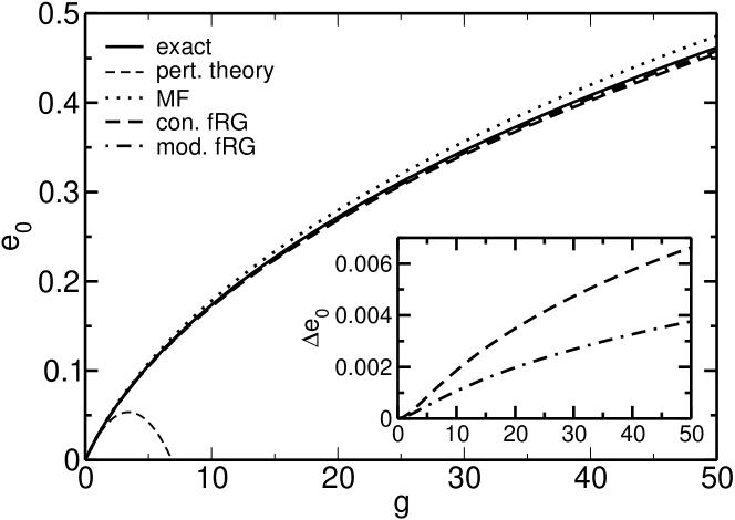
Figure 3: Coupling constant dependent part of the groundstate energy $e_{0}=E_{0}-E_{0}^{0}$ as a function of $g$. Different approximations (second order perturbation theory [thin dashed line], mean field [dotted line], conventional fRG [thick dashed line], modified fRG [dashed-dotted line]) are compared to the exact result (solid line). The inset shows the difference between the exact result and the two fRG approximations.

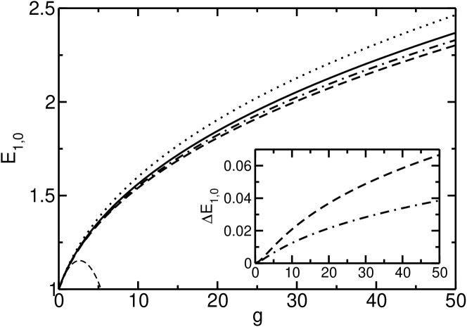
Figure 4: As in Fig. 3, but for the energy difference $E_{1,0}$ of the first excited state and the ground state.

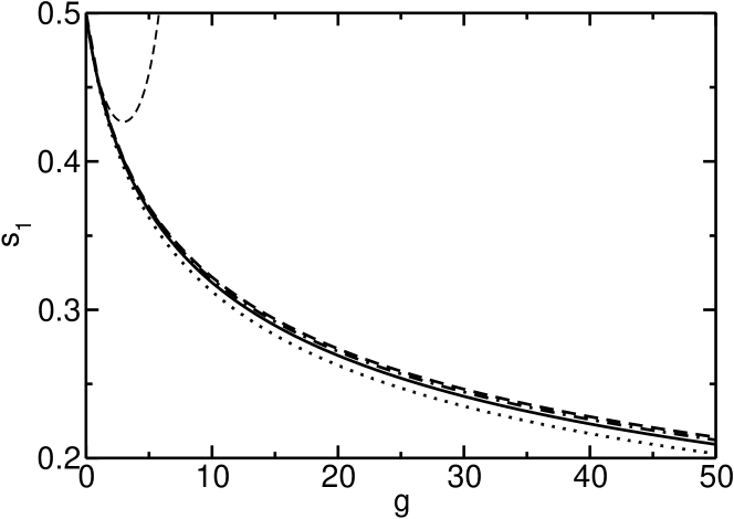
Figure 5: As in Fig. 3, but for the spectral weight $s_{1}$ of the first peak.

To numerically solve the set of differential equations (36), (37), and (3) we have discretized the frequencies (which at $T=0$ are continuous) on a linear mesh $\omega_{j}=j\delta$ with $j=-j_{0},-j_{0}+1,\ldots,j_{0}$ [22]. By increasing $j_{0}$ and decreasing $\delta$ convergence can be achieved up to the required accuracy. For our purposes $j_{0}=40$ and $\delta=0.5$ turned out to be appropriate. This leads to a set of roughly $5.3\times 10^{5}$ coupled equations. The $\Lambda$-integration is started at $\Lambda_{0}=10^{5}$ making sure that further increasing $\Lambda_{0}$ does not lead to significant changes in the results. Figs. 3 to 5 show comparisons of $e_{0}$, $E_{1,0}$, and $s_{1}$ with the different approximations considered here (second order perturbation theory, mean field, conventional fRG, modified fRG) and the exact results. Although the approximate fRGs correctly reproduce only the first two derivatives with respect to $g$ at $g=0$, they give extremely accurate results even up to $g=50$, while conventional second order perturbation theory can only be trusted for $g<1$. This provides an impressive example of the power of “renormalization group enhanced perturbation theory”. Comparing the two fRG approximations the modified scheme is roughly a factor of two closer to the exact result and thus indeed a substantial improvement [20, 23].

To avoid the problem of analytic continuation (see the next section) the results for $e_{1,0}^{\rm fRG}$ and $s_{1}^{\rm fRG}$ were obtained by fitting a function $a/(\omega^{2}+b^{2})$ with $a$ and $b$ as fitting parameters to ${\mathcal{G}}^{\rm fRG}(i\omega)=\left[\omega^{2}+1-\Sigma^{\rm fRG}(i\omega)\right]^{-1}$. Assuming this fitting form we have used that the spectral function is dominated by the first peak [21]. For the problem studied also mean field theory leads to fairly accurate results (but not as good as the fRG). This is related to the fact that low-lying eigenstates of the Hamiltonian in Eq. (29) can be described quite well by the eigenstates of a harmonic oscillator with a shifted frequency determined self-consistently.

4 Single-particle dynamics of the single impurity Anderson model

In contrast to the anharmonic oscillator studied in the previous section, the single impurity Anderson model [24]

$$H=\sum\limits_{\vec{k}\sigma}\epsilon_{\vec{k}}c^{\dagger}_{\vec{k}\sigma}c^{\phantom{\dagger}}_{\vec{k}\sigma}+\epsilon_{d}\sum\limits_{\sigma}d^{\dagger}_{\sigma}d^{\phantom{\dagger}}_{\sigma}+Ud^{\dagger}_{\uparrow}d^{\phantom{\dagger}}_{\uparrow}d^{\dagger}_{\downarrow}d^{\phantom{\dagger}}_{\downarrow}+\frac{V}{\sqrt{N}}\sum\limits_{\vec{k}\sigma}\left(c^{\dagger}_{\vec{k}\sigma}d^{\phantom{\dagger}}_{\sigma}+\mbox{h.c.}\right)$$ (42)

consists of two subsystems, namely a “conduction band” with continuous energy spectrum described by the first term in Eq. (42) and a localized level (typically referred to as “$d$”-state) with energy $\epsilon_{d}$ relative to the chemical potential $\mu$ of the conduction electrons. Two electrons occupying the localized level are in addition subject to a Coulomb repulsion $U>0$. Both subsystems are coupled via the hybridization in the last term. As the two-body interaction is restricted to a single level the SIAM falls into the of class of zero-dimensional interacting systems.

While this model looks rather simple, it contains all ingredients that make it a complicated many-body problem. The bare energy scales of the model are the bandwidth $W$ of the band electrons, the local energy $\epsilon_{d}$, the Coulomb repulsion $U$, and the bare level width generated by the hybridization, $\Delta_{0}=\pi V^{2}\rho_{c}(\mu)$, where $\rho_{c}(\epsilon)$ denotes the density of states of the conduction states which is assumed to be slowly varying. In the following we restrict ourselves to the particle-hole symmetric case $2\epsilon_{d}+U=2\mu=0$. As in the parameter regime $U/\Delta_{0}\gg 1$ the charge fluctuations on the $d$-level from the average value $1$ are small, it can effectively be described by a spin antiferromagnetically coupled to the conduction electron spin density [25], the so-called Kondo model [26]. This antiferromagnetic coupling leads to a screening of the local spin by the conduction electrons with a characteristic energy scale $\ln(T_{\rm K})\propto-1/\Delta_{0}$, the Kondo temperature. As is apparent from this expression, $T_{\rm K}$ depends non-analytically on $\Delta_{0}$, signalling the occurrence of infrared divergences in perturbation theories in $\Delta_{0}/U$ [27] and a severe problem for computational techniques, namely the task to resolve an exponentially small energy scale.

On the other hand, the physics in the regimes $T,\omega\gg T_{\rm K}$ and $T,\omega\ll T_{\rm K}$ is comparatively simple. For $T,\omega\gg T_{\rm K}$ it is governed by charge excitations with energies $\epsilon_{d}$ and $\epsilon_{d}+U$ with a life-time given by $1/(2\Delta_{0})$. In the other limit $T,\omega\ll T_{\rm K}$ it has been worked out using Wilson’s NRG [28] that the system can again be described by a Hamiltonian of the form Eq. (42), but with $U\to U^{\ast}=0$, $\epsilon_{d}\to\epsilon_{d}^{\ast}=0$ and $\Delta_{0}$ replaced by $\Delta_{0}^{\ast}\sim T_{\rm K}$. This regime has been coined “local Fermi liquid” by Nozières [27]. This effective description yields a narrow resonance at the chemical potential in the spectral function of the $d$-Green function which in the symmetric case takes the form

$$G_{dd}(i\nu)=\frac{1}{i\nu-\Delta(i\nu)-\tilde{\Sigma}(i\nu)}.$$ (43)

Here $\Delta(i\nu)=V^{2}\int d\epsilon\rho_{c}(\epsilon)/(i\nu-\epsilon)$ and $\tilde{\Sigma}$ denotes all self-energy contributions of second and higher order in $U$. As a special feature of the symmetric case, already the approximation to only keep the second order self-energy $\Sigma^{(2)}$ describes the qualitative behavior of the $d$-spectral function for different values of $U/\Delta_{0}$ correctly [27]. For $U/\Delta_{0}\ll 1$ there is a Lorentzian peak at the chemical potential with a width differing little from $\Delta_{0}$. For $U/\Delta_{0}\gg 1$ most of the spectral weight is in the high energy peaks near $\pm U/2$ with a narrow resonance at $\mu=0$. Quantitatively the width and shape of this Kondo (or Abrikosov-Suhl) resonance is described poorly using $\Sigma^{(2)}$, vanishing only $\sim\Delta_{0}/U$. From the results of Sect. 3 one expects that the application of the functional renormalization group to the SIAM leads to improvements over the direct perturbational description of the Kondo resonance. For the SIAM the fRG results can be compared to the outcome of NRG calculations [1, 28]. An important aspect of the treatment of the SIAM with the fRG is that, while the numerical effort of the NRG method increases exponentially with the number of impurity degrees of freedom, e.g. in case of additional orbital degrees of freedom or for a system of many magnetic impurities, the increase in computational resources necessary in the fRG approach described below is governed at most by a power-law.

The starting point of our fRG approach are again Eqs. (25) and (27) . We also use $m_{c}=2$, i.e. we replace the 3-particle-vertex by its initial condition $\gamma_{3}^{\Lambda}=0$, and consider $T=0$ only. We again use the frequency cutoff described in Eq. (9) and because we presently concentrate on spectral properties only flow equations for the self-energy and for the 2-particle-vertex (and not the ground state energy) will be derived. Note that the calculation of two-particle properties is possible within the same scheme without further difficulties [12] and will be discussed in a forthcoming publication.

For the SIAM all Green functions $G_{i,j}$ different from $G_{dd}$ can be expressed in terms of $G_{dd}$ and Green functions of the non-interacting system. For the calculation of $G_{dd}$ the multi-index $k$ is replaced by a spin-index $\sigma$ and a frequency $\nu$. The 2-particle-vertex can then be written as

$${\gamma}_{2}^{\Lambda}(k_{1}^{\prime},k_{2}^{\prime};k_{1},k_{2})={\delta(\nu_{1}+\nu_{2}-\nu_{1}^{\prime}-\nu_{2}^{\prime})}$$ (44)

$$\times\Bigl{\{}\displaystyle\delta_{\sigma_{1},\sigma_{1}^{\prime}}\delta_{\sigma_{2},\sigma_{2}^{\prime}}\ \mathcal{U}^{\Lambda}(i\nu_{1}^{\prime},i\nu_{2}^{\prime};i\nu_{1},i\nu_{2})-\displaystyle\delta_{\sigma_{1},\sigma_{2}^{\prime}}\delta_{\sigma_{2},\sigma_{1}^{\prime}}\ \mathcal{U}^{\Lambda}(i\nu_{2}^{\prime},i\nu_{1}^{\prime};i\nu_{1},i\nu_{2})\Bigr{\}}.$$

This can be used to perform the sum over the spins in Eq. (25) and we find for the self-energy

$$\frac{d}{d\Lambda}{\Sigma^{\Lambda}(i\nu)}=-\frac{1}{2\pi}\int_{-\infty}^{\infty}d\nu^{\prime}{\mathcal{S}^{\Lambda}(i\nu^{\prime})}\Bigl{[}2\,\mathcal{U}^{\Lambda}(i\nu,i\nu^{\prime};i\nu,i\nu^{\prime})-\mathcal{U}^{\Lambda}(i\nu^{\prime},i\nu;i\nu,i\nu^{\prime})\Bigr{]}.$$ (45)

In order to derive a flow equation for $\mathcal{U}^{\Lambda}(i\nu_{1}^{\prime},i\nu_{2}^{\prime};i\nu_{1},i\nu_{2})$, with $\nu_{2}=\nu_{1}^{\prime}+\nu_{2}^{\prime}-\nu_{1}$, the spin-sum in Eq. (27) has to be performed as well. This leads to the lengthy expression Eq. (60), presented in Appendix A.

The initial values are given by $\Sigma^{\Lambda=\infty}(i\nu)=0$ and $\mathcal{U}^{\Lambda=\infty}(i\nu_{1}^{\prime},i\nu_{2}^{\prime};i\nu_{1},i\nu_{2})=U$. In the numerical solution of these flow equations we start integrating at finite $\Lambda_{0}\gg\max(U,\Delta_{0})$. The integration from $\Lambda=\infty$ to $\Lambda_{0}$ can be performed analytically. Up to corrections of order $\Lambda_{0}^{-1}$ the new initial conditions are $\Sigma^{\Lambda_{0}}(i\nu)=U/2$ and $\mathcal{U}^{\Lambda_{0}}(i\nu_{1}^{\prime},i\nu_{2}^{\prime};i\nu_{1},i\nu_{2})=U$.

$\mathcal{S}^{\Lambda}(i\nu)$ and $\mathcal{P}_{\rm con}^{\Lambda}(i\nu,i\nu^{\prime})=\mathcal{S}^{\Lambda}(i\nu)\mathcal{G}^{\Lambda}(i\nu^{\prime})$ are calculated the same way as for the anharmonic oscillator using Eq. (38), and are given by

$${\mathcal{S}^{\Lambda}(i\nu)}\to{\delta(|\nu|-\Lambda)}\frac{1}{\left[{\mathcal{G}^{0}(i\nu)}\right]^{-1}-{\Sigma^{\Lambda}(i\nu)}}\;,$$ (46)

with $\left[{\mathcal{G}^{0}(i\nu)}\right]^{-1}=i\nu-\Delta(i\nu)-\epsilon_{d}$ and

$$\mathcal{P}_{\rm con}^{\Lambda}(i\nu,i\nu^{\prime})\to{\delta(|\nu|-\Lambda)}\frac{1}{\left[{\mathcal{G}^{0}(i\nu)}\right]^{-1}-{\Sigma^{\Lambda}(i\nu)}}\frac{{\Theta(|\nu^{\prime}|-\Lambda)}}{\left[{\mathcal{G}^{0}(i\nu^{\prime})}\right]^{-1}-{\Sigma^{\Lambda}(i\nu^{\prime})}}$$ (47)

with $\Theta(0)=1/2$. In our calculations we use the limit of an infinite bandwidth, i.e. $\Delta(i\nu)\to-i\,{\rm sign}(\nu)\,\Delta_{0}$. The results of second order perturbation theory for the self-energy can be recovered by replacing the self-energy on the rhs of Eqs. (45) and (60) and $\mathcal{U}^{\Lambda}$ on the rhs of Eq. (60) by their initial values. It turns out that the fRG version using $\mathcal{P}_{\rm con}^{\Lambda}$ gives good results for $U/\Delta_{0}<3$, but fails to provide the expected improvement compared to the use of $\Sigma^{(2)}$ for $U/\Delta_{0}>3$. This will be discussed in more detail in a forthcoming publication. For this reason we follow [20] and replace $\mathcal{P}^{\Lambda}_{\rm con}(i\nu,i\nu^{\prime})$ by $\mathcal{P}^{\Lambda}_{\rm mod}(i\nu,i\nu^{\prime})=-\mathcal{G}^{\Lambda}(i\nu^{\prime})\displaystyle\frac{d}{d\Lambda}\mathcal{G}^{\Lambda}(i\nu)$ in Eq. (60). Applying Eq. (38) yields

$$\begin{array}[]{lll}-{\mathcal{G}^{\Lambda}(i\nu^{\prime})}\displaystyle\frac{d}{d\Lambda}{\mathcal{G}^{\Lambda}(i\nu)}&\to&\displaystyle{\delta(|\nu|-\Lambda)}\frac{1}{\left[{\mathcal{G}^{0}(i\nu)}\right]^{-1}-{\Sigma^{\Lambda}(i\nu)}}\frac{{\Theta(|\nu^{\prime}|-\Lambda)}}{\left[{\mathcal{G}^{0}(i\nu^{\prime})}\right]^{-1}-{\Sigma^{\Lambda}(i\nu^{\prime})}}\\[22.76219pt] &-&\displaystyle\frac{d}{d\Lambda}{\Sigma^{\Lambda}(i\nu)}~{}\frac{{\Theta(|\nu|-\Lambda)}}{[\left[{\mathcal{G}^{0}(i\nu)}\right]^{-1}-{\Sigma^{\Lambda}(i\nu)}]^{2}}\frac{{\Theta(|\nu^{\prime}|-\Lambda)}}{\left[{\mathcal{G}^{0}(i\nu^{\prime})}\right]^{-1}-{\Sigma^{\Lambda}(i\nu^{\prime})}}.\end{array}$$ (48)

For the integration of the $T=0$-flow equations the continuous frequencies again have to be discretized. However, in contrast to the anharmonic oscillator it is not sufficient to work with a linear mesh. Because for $U/\Delta_{0}\gg 1$ the Kondo resonance is visible only on an exponentially small energy scale around the Fermi level, we use a combination of a linear and a logarithmic mesh. This enables us to recover both, the high energy as well as the low-energy physics keeping the number of frequencies to a manageable size. The numerical effort grows with the third power of the number of frequencies in the conventional version and with almost the forth power using the modified version, due to the absence of a $\delta$-function in the last term of Eq. (48).

In the fRG one naturally obtains the self-energy for imaginary frequencies. In order to calculate spectral functions, an analytic continuation to the real axis is necessary, which is known to be an ill-posed problem. Since the results from fRG are not subject to statistical errors or noise as for example quantum Monte Carlo data, we have applied the method of Padé approximation [29] to obtain $\Sigma(z)$ from $\Sigma(i\nu)$. We find that especially the low-energy part of the spectral function which contains the Kondo resonance can be reliably extracted if sufficiently many frequencies close to the Fermi level are used (see below).

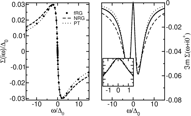
Figure 6: Left panel: $\Sigma(i\omega)$ from fRG for $U=\Delta_{0}$ (circles) compared to NRG (dashed line) and second order perturbation theory (dotted line).
Right panel: $\Im m\Sigma(\omega+i0^{+})$ for fRG obtained from Padé approximants for the data in left panel. The inset shows an enlarged view around $\omega=0$.

As an example, we present in Fig. 6 the calculated $\Sigma(i\omega)$ (left panel) and the corresponding $\Im m\Sigma(\omega+i0^{+})$ from the Padé approximation (right panel) for $U/\Delta_{0}=1$. The dashed and dotted lines represent results from NRG and second order perturbation theory, respectively. The inset in the right panel shows an enlarged view of the region around $\omega=0$. Apparently, the Padé approximation to the fRG provides reliable results, in particular around $\omega=0$, and recovers the perturbation theory as expected for such small value of $U$. Discrepancies to NRG for large $\omega$ can be traced to broadening effects in the NRG.

The true test for the method however is a comparison of the self-energy to NRG results for larger values of $U$ and in particular the behavior on low-energy scales. Such a comparison is presented in Fig. 7 for $U/\Delta_{0}=1$, $5$, and $10$. For $U/\Delta_{0}=5$ the fRG results are still in excellent agreement with the NRG data while second order perturbation theory already deviates. For $U=10\Delta_{0}$ we observe a significant dependency of the general structures and also of the slope at $\omega\to 0$ on details of the discretization mesh. It seems necessary to have an extremely fine resolution around $\omega\to 0$ and a sufficient resolution around $\omega\approx U/2$. With an exponentially vanishing low-energy scale these constraints are hard to fulfill with both linear and logarithmic meshes keeping the number of flow equations to a manageable size. The bottom left pannel contains the best fRG data we were able to obtain so far. A more extended discussion of this issue will be presented in a forthcoming publication.

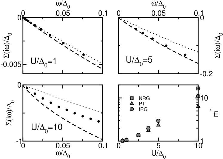
Figure 7: $\Sigma(i\omega)$ from fRG (circles) for $U/\Delta_{0}=1$, $5$ and $10$ compared to NRG (dashed line) and second order perturbation theory (dotted line).
Bottom right: Effective mass $m^{\ast}$ from fRG (circles), NRG (squares) and second order perturbation theory (triangles).

In addition to the self-energy the effective mass $m^{\ast}$ obtained from

$$m^{\ast}=1+\lim_{\omega\searrow 0}\frac{\Im m\Sigma(i\omega)}{\omega}$$

as a function of $U$ is depicted, in the bottom right panel of Fig.  7. This quantity is directly related to the Kondo temperature [27]. Compared to perturbation theory the effective mass is much closer to the very accurate values determined from the NRG.

The evolution of the spectral function of the $d$-level, $\rho_{d}(\omega)=-\frac{1}{\pi}\Im mG_{d}(\omega+i0^{+})$ for the above values of $U$ is collected in Fig. 8. The inset shows a comparison to NRG and perturbation theory for the region around $\omega=0$ at $U/\Delta_{0}=10$. One can see very nicely the development of the sharp resonance in the spectrum and the formation of the Hubbard bands with increasing $U$.

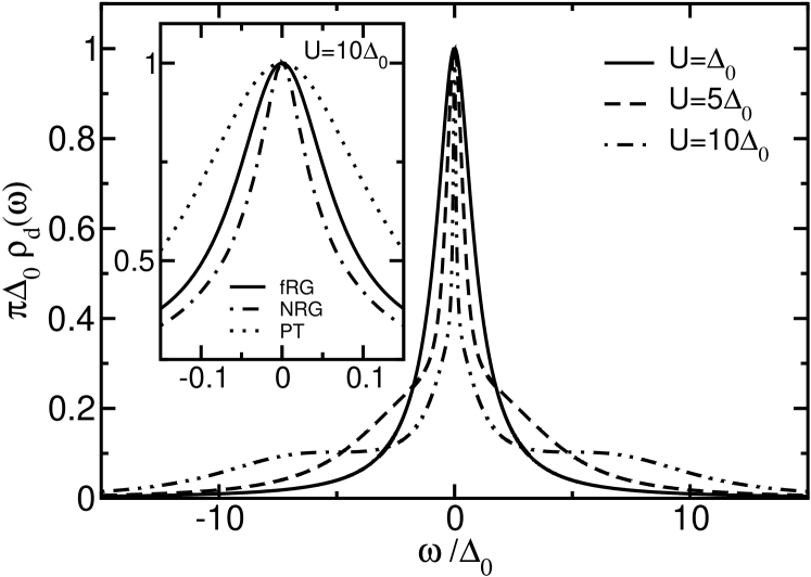
Figure 8: The evolution of the fRG spectral function for the $d$-level for the values of $U$ in Fig. 7. The inset shows a comparison to NRG for $U/\Delta_{0}=10$ for the region around $\omega=0$.

Due to the insufficient resolution at larger $\omega$ in the calculation for $U/\Delta_{0}=10$, the Hubbard bands come out too broad here. We believe that an improved discretization of the energy mesh in the solution of the flow equations will remedy that particular problem. The important region around $\omega=0$ on the other hand is captured rather well by the fRG. It is in particular noteworthy that the functional form at low frequencies (see the inset) apparently does not follow a Lorentzian but rather, like the NRG, the more complex scaling form with logarithmic tails predicted by Logan et al. [30].

5 Summary and outlook

We have presented an application of the functional renormalization group technique to solve for the dynamics of zero-dimensional interacting quantum problems. As particular examples, we discussed the anharmonic oscillator and the single impurity Anderson model. In both cases the fRG proved to be a substantial improvement over conventional low-order perturbation theory and rather close to the very accurate results obtained numerically.

We also investigated the differences between conventional fRG and a modification suggested by Katanin [20], which should improve the accuracy of the method further. That this is indeed true was shown directly for the anharmonic oscillator. For the single impurity Anderson model it was actually necessary to use this modified version to obtain sensible results for values $U/\Delta_{0}>3$.

An important aspect of the fRG is that an extension of the SIAM to more complex systems, like e.g. orbital degrees of freedom or systems of coupled impurities is straightforward. This is in principle also true for Wilson’s NRG. In the latter, however, the exponentially increasing Hilbert space renders a practical application quickly impossible. For the fRG, on the other hand, the major modification will be an increase of the number of equations, which means that the numerical effort will increase at most with a power-law. This feature makes the fRG a possible method to study features of complex impurity systems and in particular a potential “impurity solver” for mean-field theories of interacting lattice models like the Hubbard model in the framework of the dynamical mean-field theory [31] or the dynamical cluster approximation [32]. Furthermore, as it becomes clear from the anharmonic oscillator, the fRG is of equal complexity for bosonic and fermionic systems. This makes opens the possibility to study combinations of such degrees of freedom in impurity models. A question which can be addressed using the fRG is the influence of phonons or magnetic fluctuations on low energy scales. Within the dynamical mean-field theory the metal-insulator transition in the presence of phonons (Kondo volume collapse [33]) as well as the problem of non-Fermi liquid formation in for example CeCu_6-xAu_x [34] can be studied.

Appendix A

Depending on the specific parameterization of the 2-particle-vertex flow equations for the relevant frequency dependent parts of the vertex and for the self-energy can be derived by using the spin conservation on the vertex when the sum over spins in Eq. (27) is performed. For the form of the the vertex given in Eq. (44) the corresponding flow equation for the self-energy is given by Eq. (45), and the equation for the frequency dependent part of the vertex $\mathcal{U}^{\Lambda}(i\nu_{1}^{\prime},i\nu_{2}^{\prime};\nu_{1},i\nu_{2})$ with $\nu_{2}=\nu_{1}^{\prime}+\nu_{2}^{\prime}-\nu_{1}$ reads

$$\frac{d}{d\Lambda}\mathcal{U}^{\Lambda}\begin{array}[t]{l}\!\!\!\displaystyle(i\nu_{1}^{\prime},i\nu_{2}^{\prime};i\nu_{1},i\nu_{2})=-\frac{1}{2\pi}\int_{-\infty}^{\infty}d\nu\displaystyle\Biggl{[}\mathcal{P}^{\Lambda}(i\nu,i\nu_{1}+i\nu_{2}-i\nu)\\[14.22636pt] \Bigl{(}-\mathcal{U}^{\Lambda}(i\nu,i\nu_{1}+i\nu_{2}-i\nu;i\nu_{1},i\nu_{2})\mathcal{U}^{\Lambda}(i\nu_{2}^{\prime},i\nu_{1}^{\prime};i\nu_{1}+i\nu_{2}-i\nu,i\nu)\\[14.22636pt] -\mathcal{U}^{\Lambda}(i\nu_{1}+i\nu_{2}-i\nu,i\nu;i\nu_{1},i\nu_{2})\mathcal{U}^{\Lambda}(i\nu_{1}^{\prime},i\nu_{2}^{\prime};i\nu_{1}+i\nu_{2}-i\nu,i\nu)\Bigr{)}\\[14.22636pt] \displaystyle+\biggl{\{}\mathcal{P}^{\Lambda}(i\nu,-i\nu_{1}+i\nu_{1}^{\prime}+i\nu)\\[14.22636pt] \Bigl{(}2\,\mathcal{U}^{\Lambda}(i\nu_{1}^{\prime},i\nu;i\nu_{1},-i\nu_{1}+i\nu_{1}^{\prime}+i\nu)\mathcal{U}^{\Lambda}(i\nu_{2}^{\prime},-i\nu_{1}+i\nu_{1}^{\prime}+i\nu;i\nu_{2},i\nu)\\[14.22636pt] -\mathcal{U}^{\Lambda}(i\nu_{1}^{\prime},i\nu;i\nu_{1},-i\nu_{1}+i\nu_{1}^{\prime}+i\nu)\mathcal{U}^{\Lambda}(-i\nu_{1}+i\nu_{1}^{\prime}+i\nu,i\nu_{2}^{\prime};i\nu_{2},i\nu)\\[14.22636pt] -\mathcal{U}^{\Lambda}(i\nu,i\nu_{1}^{\prime};i\nu_{1},-i\nu_{1}+i\nu_{1}^{\prime}+i\nu)\mathcal{U}^{\Lambda}(i\nu_{2}^{\prime},-i\nu_{1}+i\nu_{1}^{\prime}+i\nu;i\nu_{2},i\nu)\Bigr{)}\\[14.22636pt] +(1^{\prime}\leftrightarrow 2^{\prime};1\leftrightarrow 2)\biggr{\}}\\[14.22636pt] \displaystyle-\biggl{\{}\mathcal{P}^{\Lambda}(i\nu,-i\nu_{1}+i\nu_{2}^{\prime}+i\nu)\\[14.22636pt] \mathcal{U}^{\Lambda}(i\nu,i\nu_{2}^{\prime};i\nu_{1},-i\nu_{1}+i\nu_{2}^{\prime}+i\nu)\mathcal{U}^{\Lambda}(-i\nu_{1}+i\nu_{2}^{\prime}+i\nu,i\nu_{1}^{\prime};i\nu_{2},i\nu)\\[14.22636pt] +(1^{\prime}\leftrightarrow 2^{\prime};1\leftrightarrow 2)\biggr{\}}\Biggr{]}\;.\end{array}$$ (60)

Again $\mathcal{P}$ stands either for ${\mathcal{P}}_{\rm con}$ or ${\mathcal{P}}_{\rm mod}$.

Two other possible parameterizations of the 2-particle vertex are

$${\gamma}_{2}^{\Lambda}(\xi_{1}^{\prime},\xi_{2}^{\prime};\xi_{1},\xi_{2}) = \begin{array}[t]{l}{\delta(\nu_{1}+\nu_{2}-\nu_{1}^{\prime}-\nu_{2}^{\prime})}\displaystyle\Bigl{\{}\delta_{\sigma_{1},\sigma_{2}}\delta_{\sigma_{1}^{\prime},\sigma_{2}^{\prime}}\delta_{\sigma_{1},\sigma_{1}^{\prime}}\ \mathcal{U}_{p}^{\Lambda}(i\nu_{1}^{\prime},i\nu_{2}^{\prime};i\nu_{1},i\nu_{2})\\[14.22636pt] +\displaystyle\delta_{\sigma_{1},-\sigma_{2}}\delta_{\sigma_{1}^{\prime},-\sigma_{2}^{\prime}}\ \Bigl{(}\delta_{\sigma_{1},\sigma_{1}^{\prime}}\mathcal{U}_{a}^{\Lambda}(i\nu_{1}^{\prime},i\nu_{2}^{\prime};i\nu_{1},i\nu_{2})-\delta_{\sigma_{1},-\sigma_{1}^{\prime}}\mathcal{U}_{a}^{\Lambda}(i\nu_{2}^{\prime},i\nu_{1}^{\prime};i\nu_{1},i\nu_{2})\Bigr{)}\Bigr{\}}.\end{array}$$

and

$${\gamma}_{2}^{\Lambda}(\xi_{1}^{\prime},\xi_{2}^{\prime};\xi_{1},\xi_{2})={\delta(\nu_{1}+\nu_{2}-\nu_{1}^{\prime}-\nu_{2}^{\prime})}\Bigl{\{}\begin{array}[t]{l}\displaystyle S_{\sigma_{1}^{\prime},\sigma_{2}^{\prime};\sigma_{1},\sigma_{2}}\ \mathcal{U}_{S}^{\Lambda}(i\nu_{1}^{\prime},i\nu_{2}^{\prime};i\nu_{1},i\nu_{2})\\[14.22636pt] +\displaystyle T_{\sigma_{1}^{\prime},\sigma_{2}^{\prime};\sigma_{1},\sigma_{2}}\ \mathcal{U}_{T}^{\Lambda}(i\nu_{1}^{\prime},i\nu_{2}^{\prime};i\nu_{1},i\nu_{2})\Bigr{\}}\end{array}$$

with

$$S_{\sigma_{1}^{\prime},\sigma_{2}^{\prime};\sigma_{1},\sigma_{2}}=\frac{1}{2}\left(\delta_{\sigma_{1},\sigma_{1}^{\prime}}\delta_{\sigma_{2},\sigma_{2}^{\prime}}-\delta_{\sigma_{1},\sigma_{2}^{\prime}}\delta_{\sigma_{2},\sigma_{2}^{\prime}}\right);\ T_{\sigma_{1}^{\prime},\sigma_{2}^{\prime};\sigma_{1},\sigma_{2}}=\frac{1}{2}\left(\delta_{\sigma_{1},\sigma_{1}^{\prime}}\delta_{\sigma_{2},\sigma_{2}^{\prime}}+\delta_{\sigma_{1},\sigma_{2}^{\prime}}\delta_{\sigma_{2},\sigma_{2}^{\prime}}\right)\;.$$

Both these parameterizations lead to different set of flow equations for the self-energy and to two sets of flow equations for the frequency dependent functions $\mathcal{U}_{p}^{\Lambda}$ and $\mathcal{U}_{a}^{\Lambda}$ for the first and $\mathcal{U}_{S}^{\Lambda}$ and $\mathcal{U}_{T}^{\Lambda}$ for the second (compared to one set for the parameterization Eq. (44)) implying an increased numerical effort. They are usefull to further investigate the processes occurring during the integration of the flow equations. This way we are able to distinguish the behavior of different channels of the interaction.

References

References

• [1] K.G. Wilson, Rev. Mod. Phys. 47, 773 (1975).
• [2] S.D. Glazek and P.B. Wiegmann, Phys. Rev. D 48, 5863 (1993); F. Wegner, Ann. Physik (Leipzig) 3, 77 (1994).
• [3] P. Lenz and F. Wegner, Nucl. Phys. B[FS] 482, 693 (1996); A. Mielke, Europhys. Lett. 40, 195 (1997); M. Ragwitz and F. Wegner, Eur. Phys. J. B 8, 9 (1999).
• [4] G.S. Uhrig, Phys. Rev. B 57, R14004 (1998); C. Knetter and G.S. Uhrig, Eur. Phys. J. B 13, 209 (2000).
• [5] S. Kehrein and A. Mielke, Ann. Phys. (New York) 252, 1 (1996); C. Slezak, S. Kehrein, Th. Pruschke and M. Jarrell, Phys. Rev. B 67, 184408 (2003).
• [6] J. Polchinski, Nucl. Phys. B 231, 269 (1984).
• [7] C. Wetterich, Phys. Lett. B 301, 90 (1993).
• [8] T.R. Morris, Int. J. Mod. Phys. A 9, 2411 (1994).
• [9] M. Salmhofer, Renormalization (Springer, Berlin, 1998).
• [10] As an even simpler “toy model” we have studied the classical anharmonic oscillator. Besides the one-particle irreducible version for this model we have also investigated the fRG schemes using amputated connected Green functions [6] and Wick ordered amputated connected Green functions [9]. Comparing results within the same order of truncation the irreducible scheme always led to the best results.
• [11] D. Zanchi and H.J. Schulz, Phys. Rev. B 61, 13609 (2000).
• [12] C.J. Halboth and W. Metzner, Phys. Rev. B 61, 7364 (2000).
• [13] C. Honerkamp, M. Salmhofer, N. Furukawa, and T.M. Rice, Phys. Rev. B 63, 035109 (2001).
• [14] T. Busche, L. Bartosch, and P. Kopietz, J. Phys.: Condens. Matter 14, 8513 (2002).
• [15] V. Meden, W. Metzner, U. Schollwöck, and K. Schönhammer, Phys. Rev. B 65, 045318 (2002); J. Low Temp. Phys. 126, 1147 (2002); S. Andergassen, T. Enss, V. Meden, W. Metzner, U. Schollwöck, and K. Schönhammer, cond-mat/0403517.
• [16] Certain aspects of the frequency dependence were taken into account in Ref. [14] and: C. Honerkamp and M. Salmhofer, Phys. Rev. B 67, 174504 (2003).
• [17] e.g. see C.M. Bender and T.T. Wu, Phys. Rev. 184, 1231 (1969); C.M. Bender and T.T. Wu, Phys. Rev. Lett. 27, 461 (1971); W. Janke and H. Kleinert, ibid. 75, 2787 (1995); E.J. Weniger, ibid. 77, 2859 (1996); C.M. Bender and L.M.A. Bettencourt, ibid. 77, 4114 (1996); T. Hatsuda, T. Kunihiro, and T. Tanaka, ibid. 78, 3229 (1997); Y. Meurice, ibid. 88, 141601 (2002) and references therein.
• [18] The problem has also been studied using Wegner’s flow equation technique; G. Uhrig, private communication.
• [19] J.W. Negele and H. Orland, Quantum Many-Particle Physics (Addison-Wesley, 1988).
• [20] A.A. Katanin, cond-mat/0402602.
• [21] For symmetry reasons the $s_{n}$ with even $n$ vanish. For the $g$ considered here the exact spectral weight $s_{3}$ is roughly three orders of magnitude smaller than $s_{1}$. Thus extracting more than $s_{1}^{\rm fRG}$ and $E_{1,0}^{\rm fRG}$ is beyond the accuracy of our numerical treatment of the flow equations.
• [22] This discretization is not equivalent to considering finite temperatures. Although the fRG method is set up for arbitrary $T$ (see Sect. 2) in most applications calculations were performed at $T=0$. Using a smooth frequency cutoff fRG results for finite $T$ for the problem of resonant tunneling in a Luttinger liquid are presented in: V. Meden, T. Enss, S. Andergassen, W. Metzner, and K. Schönhammer, cond-mat/0403655.
• [23] Also for the classical anharmonic oscillator compared to the conventional scheme the modified fRG [20] leads to better agreement with the exact result.
• [24] P.W. Anderson, Phys. Rev. 124, 41 (1961).
• [25] R. Schrieffer and P.A. Wolff, Phys. Rev. 149, 491 (1966).
• [26] J. Kondo, Prog. Theo. Phys. 32, 37 (1964).
• [27] A.C. Hewson in D. Edwards and D. Melville, eds., The Kondo Problem to Heavy Fermions (Cambridge University Press, 1993).
• [28] H.R. Krishnamurthy, J.W. Wilkins and K.G. Wilson, Phys. Rev. B21, 1003 (1980).
• [29] W.H. Press et al., Numerical Recipes in C (Cambridge University Press, 1993).
• [30] D. Logan and M. Glossop, J. Phys.: Condens. Matter 12, 985 (2000).
• [31] Th. Pruschke, M. Jarrell, and J.K. Freericks, Adv. in Phys. 44, 187 (1995); A. Georges, G. Kotliar, W. Krauth, and M.J. Rozenberg, Rev. Mod. Phys. 68, 13 (1996).
• [32] Th. Maier, M. Jarrell, Th. Pruschke, and M. Hettler, cond-mat/0404055 (2004).
• [33] J. W. Allen and R. M. Martin, Phys. Rev. Lett. 49, 1106, (1982); J. W. Allen and L. Z. Liu, Phys. Rev. B 46, 5047, (1992); M. Lavagna et al., Phys. Lett. 90A, 210 (1982).
• [34] J.L. Smith and Q. Si, Phys. Rev. B 61, 5184 (2000).