Numerical Contractor Renormalization Method for Quantum Spin Models

Abstract

We demonstrate the utility of the numerical Contractor Renormalization (CORE) method for quantum spin systems by studying one and two dimensional model cases. Our approach consists of two steps: (i) building an effective Hamiltonian with longer ranged interactions up to a certain cut-off using the CORE algorithm and (ii) solving this new model numerically on finite clusters by exact diagonalization and performing finite-size extrapolations to obtain results in the thermodynamic limit. This approach, giving complementary information to analytical treatments of the CORE Hamiltonian, can be used as a semi-quantitative numerical method. For ladder type geometries, we explicitely check the accuracy of the effective models by increasing the range of the effective interactions until reaching convergence. Our results in the perturbative regime and also away from it are in good agreement with previously established results. In two dimensions we consider the plaquette lattice and the kagomé lattice as non-trivial test cases for the numerical CORE method. As it becomes more difficult to extend the range of the effective interactions in two dimensions, we propose diagnostic tools (such as the density matrix of the local building block) to ascertain the validity of the basis truncation. On the plaquette lattice we have an excellent description of the system in both the disordered and the ordered phases, thereby showing that the CORE method is able to resolve quantum phase transitions. On the kagomé lattice we find that the previously proposed twofold degenerate $S=1/2$ basis can account for a large number of phenomena of the spin $1/2$ kagomé system. For spin $3/2$ however this basis does not seem to be sufficient anymore. In general we are able to simulate system sizes which correspond to an $8\times 8$ lattice for the plaquette lattice or a 48-site kagomé lattice, which are beyond the possibilities of a standard exact diagonalization approach.

Low-dimensional quantum magnets are at the heart of current interest in strongly correlated electron systems. These systems are driven by strong correlations and large quantum fluctuations - especially when frustration comes into play - and can exhibit various unconventional phases and quantum phase transitions.

One of the major difficulties in trying to understand these systems is that strong correlations often generate highly non trivial low-energy physics. Not only the groundstate of such models is generally not known but also the low-energy degrees of freedom can not be identified easily. Moreover, among the techniques available to investigate these systems, not many have the required level of generality to provide a systematic way to derive low-energy effective Hamiltonians.

Recently the Contractor Renormalization (CORE) method has been introduced by Morningstar and Weinstein weinstein96 . The key idea of the approach is to derive an effective Hamiltonian acting on a truncated local basis set, so as to exactly reproduce the low energy spectrum. In principle the method is exact in the low energy subspace, but only at the expense of having a priori long range interactions. The method becomes most useful when one can significantly truncate a local basis set and still restrict oneself to short range effective interactions. This however depends on the system under consideration and has to be checked systematically. Since its inception the CORE method has been mostly used as an analytical method to study strongly correlated systems weinstein01 ; core-bosonfermion ; core-pyrochlore . Some first steps in using the CORE approach and related ideas in a numerical framework have also been undertaken shepard97 ; dynamicCORE ; core-tJladder ; malrieu .

The purpose of the present paper is to explore the numerical CORE method as a complementary approach to more analytical CORE procedures, and to systematically discuss its performance in a variety of low dimensional quantum magnets, both frustrated and unfrustrated. The approach consists basically of numerical exact diagonalizations of the effective Hamiltonians. In this way a large number of interesting quantities are accessible, which otherwise would be hard to obtain. Furthermore we discuss some criteria and tools useful to estimate the quality of the CORE approach.

The outline of the paper is as follows: In the first section we will review the CORE algorithm in general and discuss some particularities in a numerical CORE approach, both at the level of the calculation of the effective Hamiltonians and the subsequent simulations.

In section II we move to the first applications on one-dimensional (1D) systems: the well known two-leg spin ladder and the 3-leg spin ladder with periodic boundary conditions in the transverse direction (3-leg torus). Both systems exhibit generically a finite spin gap and a finite magnetic correlation length. We will show that the numerical CORE method is able to get rather accurate estimates of the groundstate energy and the spin gap by successively increasing the range of the effective interactions.

In section III we discuss two-dimensional (2D) systems. As in 2D a long ranged cluster expansion of the interactions is difficult to achieve on small clusters, we will discuss some techniques to analyze the quality of the basis truncation. We illustrate these issues on two model systems, the plaquette lattice and the kagomé lattice. The plaquette lattice is of particular interest as it exhibits a quantum phase transition from a disordered plaquette state to a long range ordered Néel antiferromagnet, which cannot be reached by a perturbative approach. We show that a range-two effective model captures many aspects of the physics over the whole range of parameters. The kagomé lattice on the other hand is a highly frustrated lattice built of corner-sharing triangles. For spin $1/2$ it has been studied both numerically and analytically and it is one best-known candidate systems for a spin liquid groundstate. A very peculiar property is the exponentially large number of low-energy singlets in the magnetic gap. We show that already a basic range two CORE approach is able to devise an effective model which exhibits the same exotic low-energy physics. For higher half-integer spin, i.e. $S=3/2$, this simple effective Hamiltonian breaks down; we analyze how to detect this, and discuss some ways to improve the results.

In the last section we conclude and give some perspectives. Finally three appendices are devoted to (i) the density matrix of local building block, (ii) the calculation of observables by energy considerations and (iii) some general remarks on effective Hamiltonians coupling antiferromagnetic half-integer spin triangles.

I CORE Algorithm

The Contractor Renormalization (CORE) method has been proposed by Morningstar and Weinstein in the context of general Hamiltonian lattice models weinstein96 . Later Weinstein applied this method with success to various spin chain models weinstein01 . For a review of the method we refer the reader to these original papers weinstein96 ; weinstein01 and also to a pedagogical article by Altman and Auerbach core-bosonfermion which includes many details. Here, we summarize the basic steps before discussing some technical aspects which are relevant in our numerical approach.

CORE Algorithm :

• Choose a small cluster (e.g. rung, plaquette, triangle, etc) and diagonalize it. Keep $M$ suitably chosen low-energy states.

• Diagonalize the full Hamiltonian $H$ on a connected graph consisting of $N_{c}$ clusters and obtain its low-energy states $|n\rangle$ with energies $\varepsilon_{n}$.

• The eigenstates $|n\rangle$ are projected on the tensor product space of the states kept and Gram-Schmidt orthonormalized in order to get a basis $|\psi_{n}\rangle$ of dimension $M^{N_{c}}$. As it may happen that some of the eigenstates have zero or very small projection, or vanish after the orthogonalization it might be necessary to obtain more than just $M^{N_{c}}$ exact eigenstates.

• Next, the effective Hamiltonian for this graph is built as

  $$h_{N_{c}}=\sum_{n=1}^{M^{N_{c}}}\varepsilon_{n}|\psi_{n}\rangle\langle\psi_{n}|.$$ (1)

• The connected range-$N_{c}$ interactions $h^{\rm conn}_{N_{c}}$ are determined by substracting the contributions of all connected subclusters.

• Finally, the effective Hamiltonian is given by a cluster expansion as

  $$H^{\mbox{\tiny CORE}}=\sum_{i}h_{i}+\sum_{\langle ij\rangle}h_{ij}+\sum_{\langle ijk\rangle}h_{ijk}+\cdots$$ (2)

This effective Hamiltonian exactly reproduces the low-energy physics provided the expansion goes to infinity. However, if the interactions are short-range in the starting Hamiltonian, we can expect that these operators will become smaller and smaller, at least in certain situations. In the following, we will truncate at range $r$ and verify the convergence in several cases. This convergence naturally depends on the number $M$ of low-lying states that are kept on a basic block. In order to describe quantitatively how “good” these states are, we introduce the density matrix in section III.

When the number of blocks increases, a full diagonalization is not always easy and one is tempted to use a Lanczos algorithm in order to compute the low-lying eigenstates. In that case, one has to be very careful to resolve the correct degeneracies, which is known to be a difficult task in the Lanczos framework. In practice such degeneracies arise when the cluster to be diagonalized is highly symmetric. If the degeneracies are ignored, often a wrong effective Hamiltonian with broken SU(2) symmetry is obtained. As a consequence we recommend to use specialized LAPACK routines whenever possible.

In the present work we investigate mainly SU(2) invariant Heisenberg models described by the usual Hamiltonian

$$H=\sum_{\langle ij\rangle}J_{ij}\vec{S}_{i}\cdot\vec{S}_{j}$$ (3)

where the exchange constants $J_{ij}$ will be limited to short-range distances in the following. As a consequence of the SU(2) symmetry, the total spin of all states is a good quantum number. This also has some effects when calculating the effective Hamiltonian. It is possible to have situations where a low energy state has a non-zero overlap with the tensor product basis, but gets eliminated by the orthogonalization procedure because one has already exhausted all the states in one particular total spin sector by projecting states with lower energy.

Once an effective Hamiltonian has been obtained, it is still a formidable task to determine its properties. Within the CORE method different routes have been taken in the past. In their pioneering papers Morningstar and Weinstein have chosen to iteratively apply the CORE method on the preceding effective Hamiltonian in order to flow to a fixed point and then to analyze the fixed point. A different approach has been taken in Refs. [core-bosonfermion, ; core-pyrochlore, ]: There the effective Hamiltonian after one or two iterations has been analyzed with mean-field like methods and interesting results have been obtained. Yet another approach - and the one we will pursue in this paper - consists of a single CORE step to obtain the effective Hamiltonian, followed by a numerical simulation thereof. This approach has been explored in a few previous studies shepard97 ; dynamicCORE ; core-tJladder . The numerical technique we employ is the Exact Diagonalization (ED) method based on the Lanczos algorithm. This technique has easily access to many observables and profits from the symmetries and conservation laws in the problem, i.e. total momentum and the total $S^{z}$ component. Using a parallelized program we can treat matrix problems of dimensions up to $\sim 50$ millions, however the matrices contain significantly more matrix elements than the ones of the microscopic Hamiltonian we start with.

II Ladder geometries

In this section, we describe results obtained on ladder systems with 2 and 3 legs respectively.

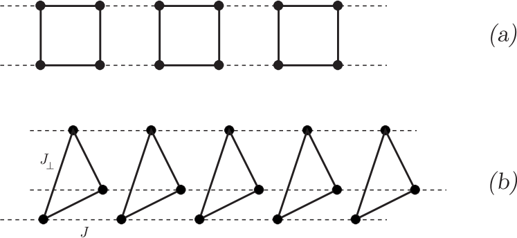
Figure 1: (a) 2-leg ladder. Basic block is a $2\times 2$ plaquette. (b) 3-leg torus with rung coupling $J_{\perp}$ and inter-rung coupling $J_{\parallel}$.

We want to build an effective model that is valid from a perturbative regime to the isotropic case $J_{ij}=J=1$. We have chosen periodic boundary conditions (PBC) along the chains in order to improve the convergence to the thermodynamic limit.

II.1 Two-leg Heisenberg ladder

The 2-leg Heisenberg ladder has been intensively studied and is known to exhibit a spin gap for all couplings 2leg ; 2legdata .

In order to apply our algorithm, we select a $2\times 2$ plaquette as the basic unit (see Fig. 1 (a)). The truncated subspace is formed by the singlet ground-state (GS) and the lowest triplet state.

Using the same CORE approach, Piekarewicz and Shepard have shown that quantitative results can be obtained within this restricted subspace shepard97 . Moreover, dynamical quantities can also be computed in this framework dynamicCORE .

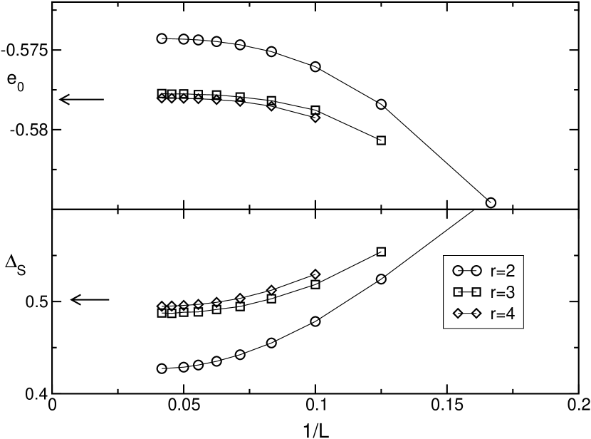
Figure 2: Ground-state energy per site and spin gap of a $2\times L$ Heisenberg ladder using CORE method with various range $r$ using PBC. For comparison, we plot the best known extrapolations 2legdata with arrows.

Since we are dealing with a simple system, we can compute the effective models including rather long-range interactions (typically, to obtain range-4 interactions, we need to compute the low-lying states on a $2\times 8$ lattice with Open Boundary Conditions which is feasible, although it requires a large numerical effort). It is desirable to compute long-range effective interactions since we wish to check how the truncation affect the physical results and how the convergence is reached.

In a second step, for each of these effective models, we perform a standard Exact Diagonalization (ED) using the Lanczos algorithm on finite clusters up to $N_{c}=12$ clusters ($N=48$ sites for the original model). The GS energy and the spin gap are shown in Fig. 2. The use of PBC allows to reduce considerably finite-size effects since we have an exponential convergence as a function of inverse length. CORE results are in perfect agreement with known results and the successive approximations converge uniformly to the exact results. For instance, the relative errors of range-4 results are $10^{-4}$ for the GS energy and $10^{-2}$ for the spin gap. This fast convergence is probably due to the rather short correlation length in an isotropic ladder (typically 3 to 4 lattice spacings xi_2leg ).

II.2 3-leg Heisenberg torus

As a second example of ladder geometry, we have studied a 3-leg Heisenberg ladder with PBC along the rungs. This property causes geometric frustration which leads to a finite spin-gap and finite dimerization for all interchain coupling $J_{\perp}$ kawano97 ; cabra98 , contrary to the open boundary condition case along the rungs, which is in the universality class of the Heisenberg chain.

Perturbation theory : The simple perturbation theory is valid when the coupling along the rung ($J_{\perp}$) is much larger than between adjacent rungs ($J_{\parallel}$). In the following, we fix $J_{\perp}=1$ as the energy unit and denote $\alpha=J_{\parallel}/J_{\perp}$.

On a single rung, the low-energy states are the following degenerate states, defined as

$$\mid\uparrow L\rangle = \frac{1}{\sqrt{3}}(\mid\uparrow\uparrow\downarrow\rangle+\omega\mid\uparrow\downarrow\uparrow\rangle+\omega^{2}\mid\downarrow\uparrow\uparrow\rangle),$$ (4)

$$\mid\downarrow L\rangle = \frac{1}{\sqrt{3}}(\mid\downarrow\downarrow\uparrow\rangle+\omega\mid\downarrow\uparrow\downarrow\rangle+\omega^{2}\mid\uparrow\downarrow\downarrow\rangle),$$

$$\mid\uparrow R\rangle = \frac{1}{\sqrt{3}}(\mid\uparrow\uparrow\downarrow\rangle+\omega^{2}\mid\uparrow\downarrow\uparrow\rangle+\omega\mid\downarrow\uparrow\uparrow\rangle),$$

$$\mid\downarrow R\rangle = \frac{1}{\sqrt{3}}(\mid\downarrow\downarrow\uparrow\rangle+\omega^{2}\mid\downarrow\uparrow\downarrow\rangle+\omega\mid\uparrow\downarrow\downarrow\rangle)$$

where $\omega=\exp(i2\pi/3)$. The indices $L$ and $R$ represent the momentum of the 3-site ring $k_{y}=2\pi/3$ and $-2\pi/3$ respectively. They define two chiral states which can be viewed as pseudo-spin states with operators $\vec{\tau}$ on each rung defined by

$$\tau^{+}\mid\cdot\,R\rangle=0\qquad\tau^{+}\mid\cdot\,L\rangle=|\cdot\,R\rangle$$

$$\tau^{-}\mid\cdot\,R\rangle=|\cdot\,L\rangle\qquad\tau^{-}\mid\cdot\,L\rangle=0$$

$$\tau^{z}\mid\cdot\,R\rangle=\frac{1}{2}\mid\cdot\,R\rangle\quad\tau^{z}\mid\cdot\,L\rangle=-\frac{1}{2}\mid\cdot\,L\rangle$$

These states have in addition a physical spin 1/2 described by $\vec{\sigma}$.

Applying the usual perturbation theory for the inter-rung coupling, one findsschulz ; kawano97

$$H_{pert}=-\frac{N}{4}+\frac{\alpha}{3}\sum_{\langle ij\rangle}\vec{\sigma}_{i}\cdot\vec{\sigma}_{j}(1+4(\tau_{i}^{+}\tau_{j}^{-}+\tau_{i}^{-}\tau_{j}^{+}))$$ (5)

where $N$ is the total number of sites.

This effective Hamiltonian has been studied with DMRG and ED techniques and it exhibits a finite spin gap $\Delta_{S}=0.28~{}J_{\parallel}$ and a dimerization of the ground state kawano97 ; cabra98 .

Here we want to use the CORE method to extend the perturbative Hamiltonian with an effective Hamiltonian in the same basis for any coupling.

CORE approach : As a basic unit, we choose a single 3-site rung. The subspace consists of the same low-energy states as for the perturbative result (Eq. (4)) which are 4-fold degenerate (2 degenerate $S=1/2$ states). We can apply our procedure to compute the effective interactions at various ranges, in order to be able to test the convergence of the method.

First, we write down the range-2 contribution under the most general form which preserves both $SU(2)$ (spin) symmetry and simultaneous translation or reflection along all the rungs :

$$H_{r=2}=Na_{0}+\sum_{\langle ij\rangle}(b_{0}\tau_{i}^{z}\tau_{j}^{z}+c_{0}(\tau_{i}^{+}\tau_{j}^{-}+\tau_{i}^{-}\tau_{j}^{+}))$$

$$+\vec{\sigma}_{i}\cdot\vec{\sigma}_{j}(a_{1}+b_{1}\tau_{i}^{z}\tau_{j}^{z}+c_{1}(\tau_{i}^{+}\tau_{j}^{-}+\tau_{i}^{-}\tau_{j}^{+}))$$ (6)

In the perturbative regime given in (5), the only non-vanishing coefficients are given by : $a_{0}=-1/4$, $a_{1}=\alpha/3$ and $c_{1}=4\alpha/3$.

The parameters of the effective Hamiltonian can be obtained and their dependence as a function of the inter-rung coupling $\alpha$ is shown in Fig. 3. We immediately see some deviations from the perturbative result since coefficients in panel (i) and (ii) are non-zero and become as important as the other terms in the isotropic limit. Surprisingly, we observe that $c_{1}$ follows its perturbative expression on the whole range of couplings whereas $a_{1}$ deviates strongly as one goes to the isotropic case but does not change sign.

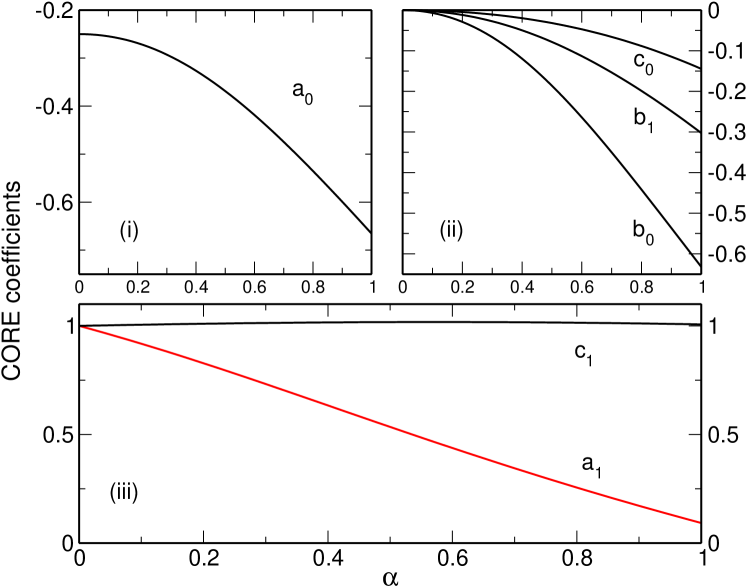
Figure 3: CORE coefficients (see Eq. 6) for two coupled triangles as a function of the inter-rung coupling $\alpha=J_{\parallel}/J_{\perp}$. The parameters were computed using range-2 CORE. The coefficients in panel (iii) have been divided by their values in the perturbative limit. They therefore all start at 1.

In order to study how the physical properties evolve as a function of $J_{\parallel}/J_{\perp}$, we have computed the GS energy and the spin gap both for a small-coupling case and in the isotropic limit, up to range 5 in the effective interactions.

Small interrung coupling : We have chosen $J_{\parallel}/J_{\perp}=0.25$ which corresponds to a case where perturbation theory should still apply. Using ED, we can solve the effective models on finite lattices and on Fig. 4, we plot the scaling of the GS energy and of the spin gap as a function of the system length $L$. Even for this rather small value of $J_{\parallel}/J_{\perp}$, our effective Hamiltonian can be considered as an improvement over the first order perturbation theory. Moreover, we observe a fast convergence with the range of interactions and already the range-3 approximation is almost indistinguishable from ED results.

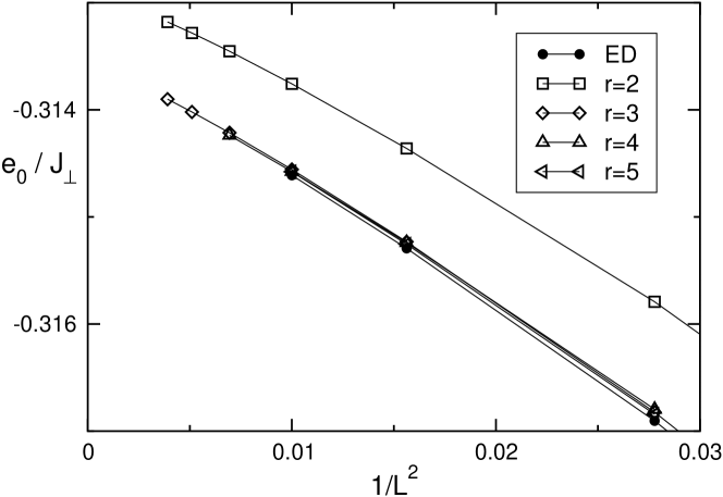
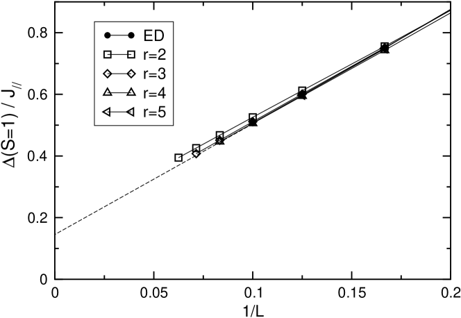
Figure 4: GS energy per site and spin gap for a $3\times L$ Heisenberg torus with $J_{\parallel}/J_{\perp}=0.25$. Results are obtained using the CORE method at various range $r$.

The estimated gap is $0.16J_{\parallel}$ and correspond to a lower bound since ultimately the gap should converge exponentially to its thermodynamic value. Our value is consistent with the DMRG one kawano97 ($\sim 0.2J_{\parallel}$), and is already reduced compared to the strong coupling result kawano97 ($\Delta_{S}=0.28J_{\parallel}$).

Isotropic case : We apply the same procedure in the isotropic limit. As expected, the convergence with the range of interactions is much slower than in the perturbative regime. We show on Fig. 5 that indeed the ground state energy converges slowly and oscillates around the correct value. These oscillations come from the fact that, in order to compute range-$r$ interactions, one has to study alternatively clusters with an even or odd number of sites. Since this system has a tendency to form dimers on nearest-neighbour bonds, it is better to compute clusters with an even number of sites.

For the spin gap, we find accurate results even with limited range interactions. In particular, we find that frustration induces a finite spin gap $\simeq 0.11~{}J_{\parallel}$ in that system. As in the previous case, this is a lower bound which is in perfect agreement with DMRG study kawano97 .

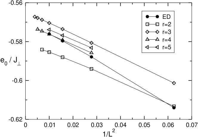
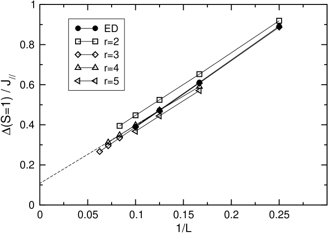
Figure 5: Same as Fig. 4 for the isotropic case $J_{\parallel}=J_{\perp}=1$.

Moreover, we find that the singlet gap vanishes in the thermodynamic limit as $1/L^{2}$ (data not shown). This singlet state at momentum $\pi$ along the chains corresponds to the state built in the generalized Lieb-Schultz-Mattis argument LSM . Here, the physical picture is a two-fold degenerate GS due to the appearance of spontaneous dimerization.

Spinon dispersion relation for the spin tube : One of the advantages of this method is to be able to get information on some quantum numbers (number of particles, magnetization, momentum…) For example, the effective Hamiltonian $H_{\rm eff}$ still commutes with translations along the legs, with the total $S^{tot}_{z}$ and $\tau_{z}$ so that we can work in a given momentum sector $(k_{x},k_{y})$ with a fixed magnetization $S^{tot}_{z}$. By computing the energy in each sector, we can compute the dispersion relation.

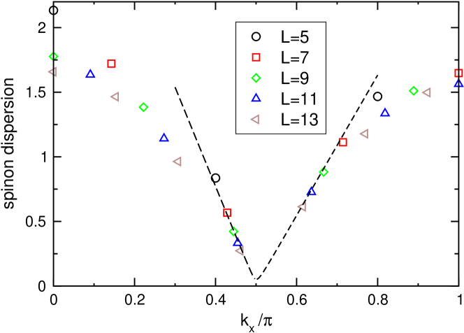
Figure 6: Spinon dispersion relation (see text) as a function of longitudinal momentum (in units of $\pi$). We only plot the lowest branch corresponding to $k_{y}=\pm 2\pi/3$. The odd lengths run from 5 to 13. The lines are guide to the eyes for an extrapolation on both sides of $\pi/2$.

In order to try to identify if the fundamental excitation is a spinon, we compute the energy difference between the lowest $S=1/2$ state when the length is odd ($L=2p+1$) and the extrapolated GS energy obtained from the data on systems with even length $2p$ and $2p+2$. The data are taken from CORE with range-4 approximation. On Fig. 6, we plot this dispersion as a function of the longitudinal momentum, relative to the GS with $L=2p$.

We observe a dispersion compatible with a spinon-like dispersion, which is massive with a gap at $\pi/2$ $\simeq 0.05\simeq\Delta_{S}/2$. This result is consistent with a picture in which the triplet excitation $\Delta_{S}$ is made of two elementary spinons. With our precision, it seems that the spinons are not bound but we cannot exclude a small binding energy.

We have on overall agreement with results obtained in the strong interchain coupling regime cabra98 .

Therefore, with CORE method, we have both the advantage of working in the reduced subspace and not being limited to the perturbative regime. Amazingly, we have observed that for a very small effort (solving a small cluster), the effective Hamiltonian gives much better results (often less than 1% on GS energies) than perturbation theory. It also gives an easier framework to systematically improve the accuracy by including longer range interactions.

For these models, the good convergence of CORE results may be due to the fact that the GS in the isotropic limit is adiabatically connected to the perturbative one. In the following part we will therefore study 2D models where a quantum phase transition occurs as one goes from the perturbative to the isotropic regime.

III Two dimensional spin models

In this section we would like to discuss the application of the numerical CORE method to two dimensional quantum spin systems. We will present spectra and observables and also discuss a novel diagnostic tool - the density matrix of local objects - in order to justify the truncation of the local state set.

One major problem in two dimension is the more elaborate cluster expansion appearing in the CORE procedure. Especially our approach based on numerical diagonalization of the resulting CORE Hamiltonian faces problems once the CORE interaction clusters wrap around the boundary of the finite size clusters. We therefore try to keep the range of the interactions minimal, but we still demand a reasonable description of low energy properties of the system. We will therefore discuss some ways to detect under what circumstances the low-range approximations fail and why.

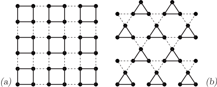
Figure 7: (a) The plaquette lattice. Full lines denote the plaquette bonds $J$, dashed lines denote the inter-plaquette coupling $J^{\prime}$. (b) The trimerized kagomé lattice. Full lines denote the up-triangle $J$ bonds, dashed lines denote the down-triangle coupling $J^{\prime}$. The standard kagomé lattice is recovered for $J^{\prime}/J=1$.

As a first example we discuss the plaquette lattice [Fig. 7 (a)], which exhibits a quantum phase transition from a gapped plaquette-singlet state with only short ranged order to a long range ordered antiferromagnetic state as a function of the interplaquette coupling KogaSigmaModelPlaquette ; KogaSeriesPlaquette ; AMLShastry ; VoigtED . We will show that the CORE method works particularly well for this model by presenting results for the excitation spectra and the order parameter. It is also a nice example of an application where the CORE method is able to correctly describe a quantum phase transition, thus going beyond an augmented perturbation scheme.

The second test case is the highly frustrated kagomé lattice [Fig. 7 (b)] with non-integer spin, which has been intensively studied for $S=1/2$ during the last few years LeungElser ; Lecheminant ; Waldtmann ; MilaPRL ; MambriniMila . Its properties are still not entirely understood, but some of the features are well accepted by now: There is no simple local order parameter detectable, neither spin order nor valence bond crystal order. There is probably a small spin gap present and most strikingly an exponentially growing number of low energy singlets emerges below the spin gap. We will discuss a convenient CORE basis truncation which has emerged from a perturbative point of view Subrahmanyam ; MilaPRL ; Raghu and consider an extension of this basis for higher non-integer spin.

III.1 Plaquette lattice

The CORE approach starts by choosing a suitable decomposition of the lattice and a subsequent local basis truncation. In the plaquette lattice the natural decomposition is directly given by the uncoupled plaquettes. Among the 16 states of an isolated plaquette we retain the lowest singlet [$K=(0,0)$] and the lowest triplet [$K=(\pi,\pi)$]. The standard argument for keeping these states relies on the fact that they are the lowest energy states in the spectrum of an isolated plaquette.

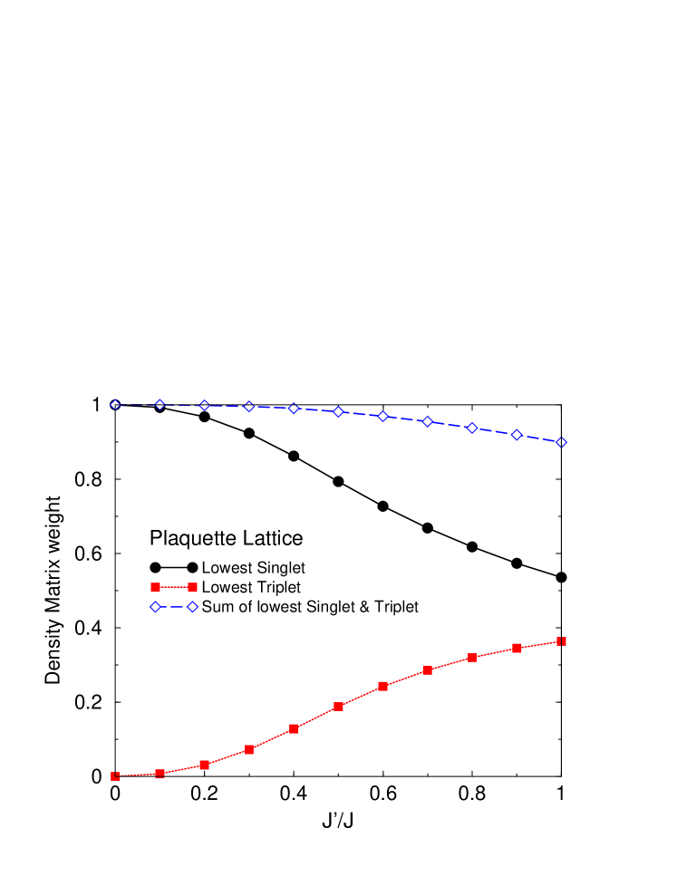
Figure 8: Density matrix weights of the two most important states on a strong ($J$-bonds) plaquette as a function of $J^{\prime}/J$. These results were obtained by ED with the original Hamiltonian on a $4\times 4$ cluster.

As discussed in appendix A, the density matrix of a plaquette in the fully interacting system gives clear indications whether the basis is suitably chosen. In Fig. 8 we show the evolution of the density matrix weights of the lowest singlet and triplet as a function of the interplaquette coupling. Even though the individual weights change significantly, the sum of both contributions remains above 90% for all $J^{\prime}/J\leq 1$. We therefore consider this a suitable choice for a successful CORE application.

A next control step consists in calculating the spectrum of two coupled plaquettes, and one monitors which states are targeted by the CORE algorithm. We show this spectrum in Fig. 9 along with the targeted states. We realize that the 16 states of our tensor product basis cover almost all the low energy levels of the coupled system. There are only two triplets just below the $S=2$ multiplet which are missed.

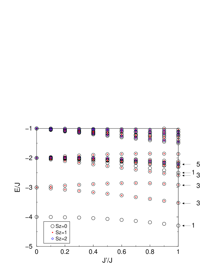
Figure 9: Low energy spectrum of two coupled plaquettes. The states targeted by the CORE algorithm are indicated by arrows together with their $SU(2)$ degeneracy.

In a first application we calculate the spin gap for different system sizes and couplings $J^{\prime}/J$. The results shown in Fig. 10 indicate a reduction of the spin gap for increasing $J^{\prime}/J$. We used a simple finite size extrapolation in $1/N$ in order to assess the closing of the gap. The extrapolation levels off to a small value for $J^{\prime}/J\geq 0.6$. The appearance of a small gap in this known gapless region is a feature already present in ED calculation of the original model VoigtED , and therefore not an artefact of our method. It is rather obvious that the triplet gap is not a very accurate tool to detect the quantum phase transition within our numerical approach. We will see later that order parameter susceptibilities are much more accurate.

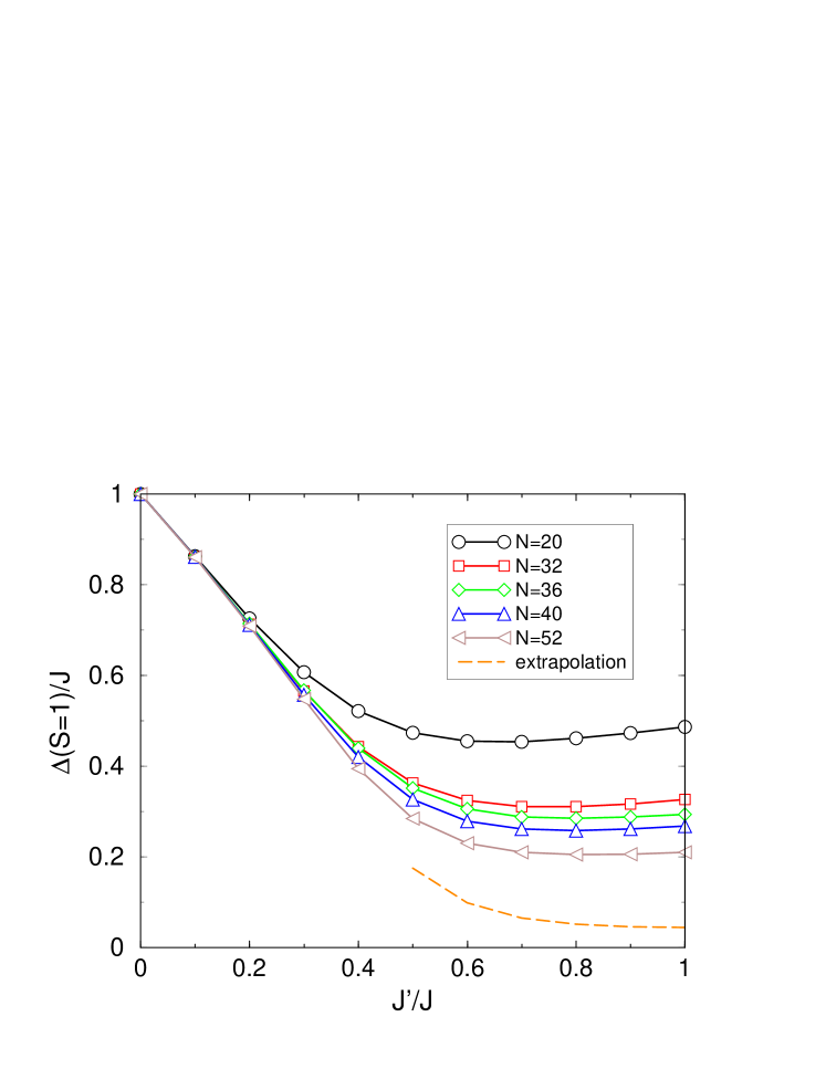
Figure 10: Triplet Gap for effective system sizes between 20 and 52 sites, as a function of the interplaquette coupling $J^{\prime}/J$. For $J^{\prime}/J\geq 0.5$ a simple extrapolation in $1/N$ is also displayed. These results compare very well with ED results on the original model [VoigtED, ].

It is well known that the square lattice $(J^{\prime}/J=1)$ is Néel ordered. One possibility to detect this order in ED is to calculate the so-called tower of excitation, i.e. the complete spectrum as a function of $S(S+1)$, $S$ being the total spin of an energy level. In the case of standard collinear Néel order a prominent feature is an alignment of the lowest level for each $S$ on a straight line, forming a so called “Quasi-Degenerate Joint States” (QDJS) ensemble TowerTriangular , which is clearly separated from the rest of the spectrum on a finite size sample. We have calculated the tower of states within the CORE approach (Fig. 11). Due to the truncated Hilbert space we cannot expect to recover the entire spectrum. Surprisingly however the CORE tower of states successfully reproduces the general features observed in ED calculations of the same model TowerEDSquare : (a) a set of QDJS with the correct degeneracy and quantum numbers (in the folded Brillouin zone); (b) a reduced number of magnon states at intermediate energies, both set of states rather well separated from the high energy part of the spectrum. While the QDJS seem not to be affected by the CORE decimation procedure, clearly some the magnon modes get eliminated by the basis truncation.

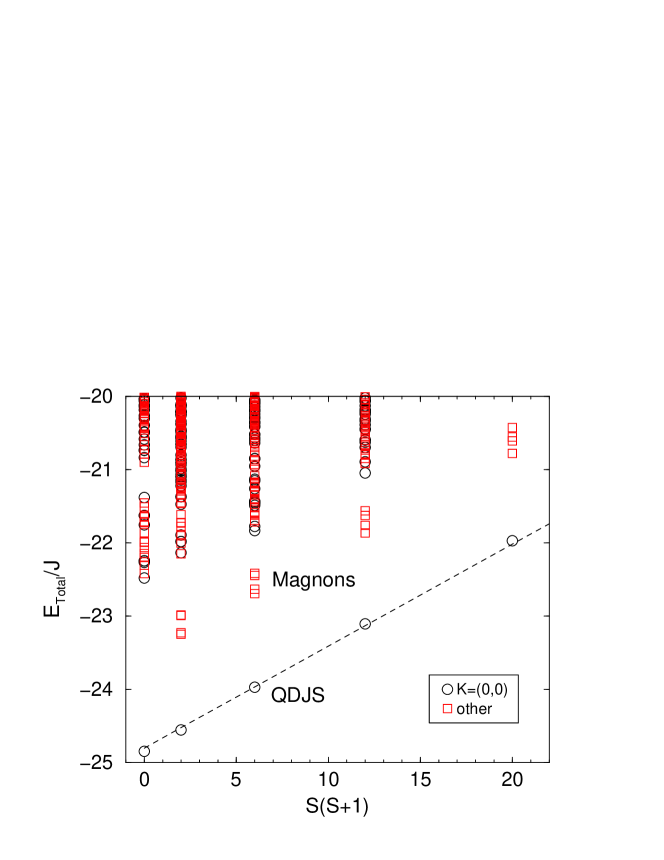
Figure 11: Tower of states obtained with a range-2 CORE Hamiltonian on an effective $N=36$ square lattice (9-site CORE cluster) in different reduced momentum sectors. The tower of states is clearly separated from the decimated magnons and the rest of the spectrum.

In order to locate the quantum phase transition from the paramagnetic, gapped regime to the Néel ordered phase, a simple way to determine the onset of long range order is desireable. We chose to directly couple the order parameter to the Hamiltonian and to calculate generalized susceptibilities by deriving the energy with respect to the external coupling. This procedure is detailed in appendix B. Its simplicity relies on the fact that only eigenvalue runs are necessary. Similar approaches have been used so far in ED and QMC calculations calandra00 ; capriotti .

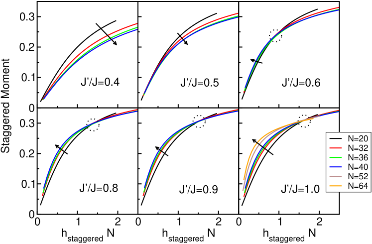
Figure 12: Staggered moment per site as a function of the rescaled applied staggered field for the plaquette lattice and different values of $J^{\prime}/J$. Circles denote the approximate crossing point of curves for different system sizes. We take the existence of this crossing as a phenomenological indication for the presence of Néel LRO. In this way the phase transition is detected between $0.5<J^{\prime}_{c}/J<0.6$, consistent with previous estimates. The arrows indicate curves for increasing system sizes.

Our results in Fig. 12 show the evolution of the staggered moment per site in a rescaled external staggered field for different inter-plaquette couplings $J^{\prime}$ and different system sizes (up to $8\times 8$ lattices). We note the appearance of an approximate crossing of the curves for different system sizes, once Néel LRO sets in. This approximate crossing relies on the fact that the slope of $m_{L}(hN)$ diverges with increasing $N$ in the ordered phase in our case capriotti . We then consider this crossing feature as an indication of the phase transition and obtain a value of the critical point $J_{c}/J=0.55\pm 0.05$. This estimate is in good agreement with previous studies using various methods KogaSeriesPlaquette ; AMLShastry ; VoigtED . We have checked the present approach by performing the same steps on the two leg ladder discussed in section II.1 and there was no long range magnetic order present, as expected.

III.2 kagomé systems with half-integer spins

In the past 10 years many efforts have been devoted to understand the low energy physics of the kagomé antiferromagnet (KAF) for spins $1/2$ LeungElser ; Lecheminant ; Waldtmann ; MilaPRL ; MambriniMila . At the theoretical level, the main motivation comes from the fact that this model is the only known example of a two-dimensional Heisenberg spin liquid. Even though many questions remain open, some very exciting low-energy properties of this system have emerged. Let us summarize them briefly: (i) the GS is a singlet ($S=0$) and has no magnetic order. Moreover no kind of more exotic ordering (dimer-dimer, chiral order, etc.) have been detected using unbiased methods; (ii) the first magnetic excitation is a triplet ($S=1$) separated from the GS by a rather small gap of order $J/20$; (iii) more surprisingly the spectrum appears as a continuum of states in all spin sectors. In particular the spin gap is filled with an exponential number of singlet excitations: ${\cal N}_{\rm singlets}\sim 1.15^{N}$; (iv) the singlet sector of the KAF can be very well reproduced by a short-range resonating valence bond approach involving only nearest-neighbor dimers.

From this point of view, the spin $1/2$ KAF with its highly unconventional low-energy physics appears to be a very sharp test of the CORE method. The case of higher half-integer spins $S=3/2,5/2\dots$ KAF is also of particular interest, since it is covered by approximative experimental realizations SCGO . Even if some properties of these experimental systems are reminiscent of the spin $1/2$ KAF theoretical support is still lacking for higher spins due to the increased complexity of these models.

In this section we discuss in detail the range-two CORE Hamiltonians for spin 1/2 and 3/2 KAF considered as a set of elementary up-triangles with couplings $J$, coupled by down-triangles with couplings $J^{\prime}$ [see Fig. 7 (b)]. The coupling ratio will be denoted by $\alpha=J^{\prime}/J$. Before going any further into the derivation of the CORE effective Hamiltonian let us start with the conventional degenerate perturbation theory results. Note that in the perturbative regime these two approaches yield the same effective Hamiltonian.

As described in Appendix C, the most general two-triangle effective Hamiltonian involving only the two spin 1/2 degrees of freedom on each triangle can be written in the following form:

$${\cal H}=Na_{0}(\alpha)+\sum_{\langle i,j\rangle} (b_{0}(\alpha)\vec{\tau}_{i}.\vec{e}_{ij}\vec{\tau}_{j}.\vec{e}_{ij}$$

$$+a_{1}(\alpha)\vec{\sigma}_{i}.\vec{\sigma}_{j}$$

$$+b_{1}(\alpha)\vec{\sigma}_{i}.\vec{\sigma}_{j}(\vec{\tau}_{i}.\vec{e}_{ij})(\vec{\tau}_{j}.\vec{e}_{ij})$$

$$+c_{1}(\alpha)\vec{\sigma}_{i}.\vec{\sigma}_{j}(\vec{\tau}_{i}.\vec{e}_{ij}+\vec{\tau}_{j}.\vec{e}_{ij})).$$

In the spirit of Mila’s approach MilaPRL for spin $1/2$ the first order perturbative Hamiltonian in $\alpha$ can easily be extended to arbitrary half-integer spin $S$:

$${\cal H}^{\rm pert.} = \frac{\alpha}{9}\vec{\sigma}_{i}.\vec{\sigma}_{j}$$

$$\times\left(1-2(2S+1)\vec{\tau}_{i}.\vec{e}_{a}\right)\left(1-2(2S+1)\vec{\tau}_{j}.\vec{e}_{b}\right)$$

and the coefficients of (III.2) in the perturbative limit are given as $a_{1}(\alpha)=\frac{\alpha}{9}$, $b_{1}(\alpha)=\frac{4\alpha}{9}(2S+1)^{2}$, $c_{1}(\alpha)=-\frac{2\alpha}{9}(2S+1)$ and $a_{0}(\alpha)=b_{0}(\alpha)=0$.

III.2.1 Choice of the CORE basis

As discussed in the previous paragraph we keep the two degenerate $S=1/2$ doublets on a triangle for the CORE basis. In analogy to the the plaquette lattice we calculate the density matrix of a single triangle embedded in a 12 site kagomé lattice for both spin $S=1/2$ and $S=3/2$, in order to get information on the quality of the truncated basis. The results displayed in Fig. 13 show two different behaviors: while the targeted states exhaust 95% for the $S=1/2$ case, they cover only $\approx$ 55% in the $S=3/2$ case. This can be considered a first indication that the range-two approximation in this basis might break down for $S>1/2$ half integer spin, while the approximation seems to work particularly well for $S=1/2$, thereby providing independent support for the adequacy of the basis chosen in a related mean-field study MilaPRL .

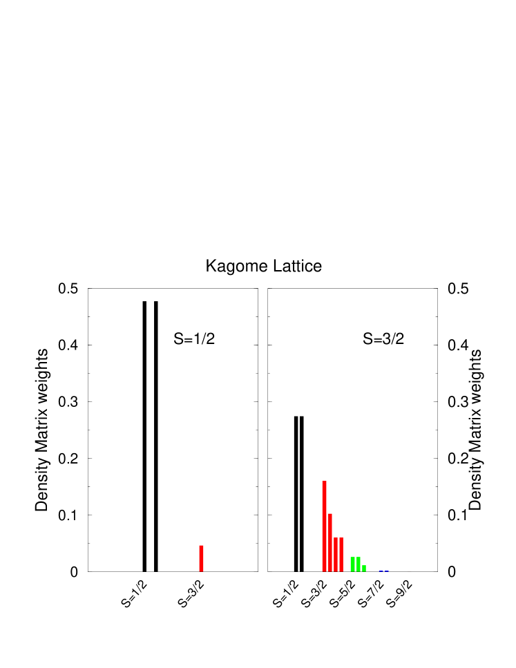
Figure 13: Density matrix weights of the different total spin states in a triangle of a 12 site kagomé cluster with $S=1/2$ and $S=3/2$ spins. These results are obtained for the homogeneous case $\alpha=1$.

We continue the analysis of the CORE basis by monitoring the evolution of the spectra of two coupled triangles in the kagomé geometry (c.f. Fig. 22) as a function of the inter-triangle coupling $J^{\prime}$, as well as the states selected by the range-two CORE algorithm. The spectrum for the spin $S=1/2$ case is shown in Fig. 14. We note the presence of a clear gap between the 16 lowest states – correctly targeted by the CORE algorithm – and the higher lying bands. This can be considered an ideal case for the CORE method. Based on this and the results of the density matrix we expect the CORE range-two approximation to work quite well.

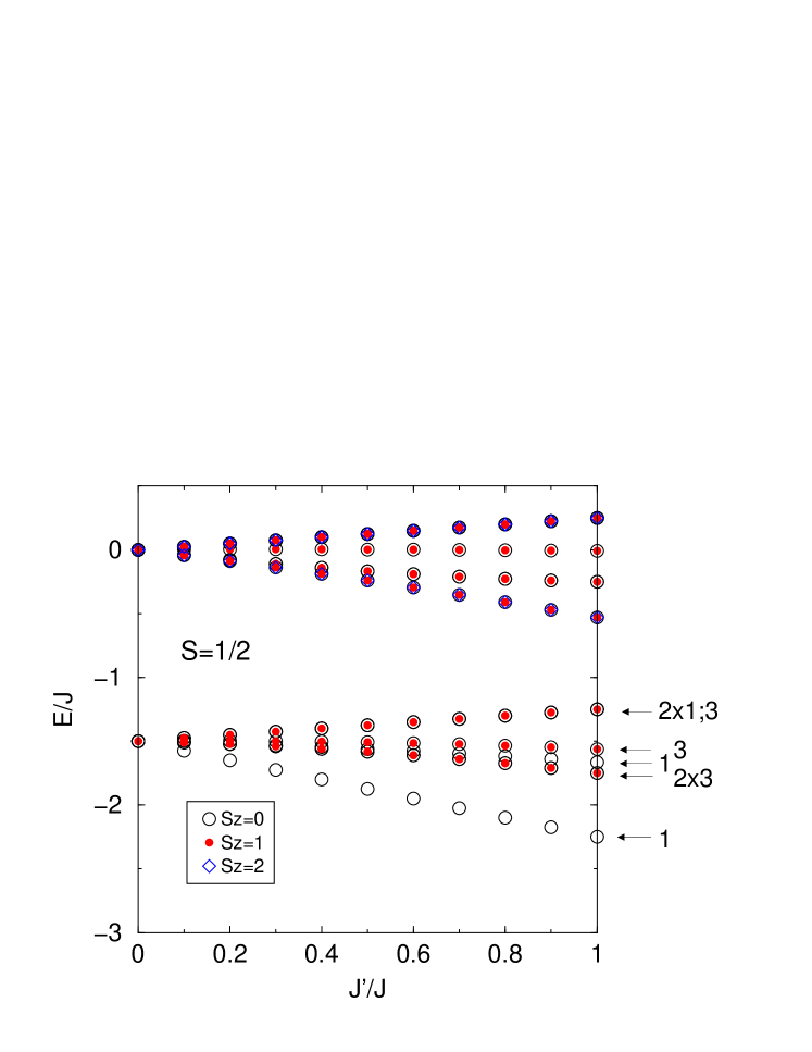
Figure 14: Spectrum of two coupled triangles in the kagomé geometry with $S=1/2$ spins. The entire lowest band containing 16 states is successfully targeted by the CORE algorithm.

We compare these encouraging results with the spectrum for the spin $S=3/2$ case displayed in Fig. 15. Here the situation is less convincing: very rapidly $(J^{\prime}/J\gtrsim 0.45)$ the low energy states mix with originally higher lying states and the CORE method continues to target two singlets which lie high up in energy when reaching $J^{\prime}/J=1$. We expect this to be a situation where the CORE method will probably not work correctly when restricted to range-two terms only.

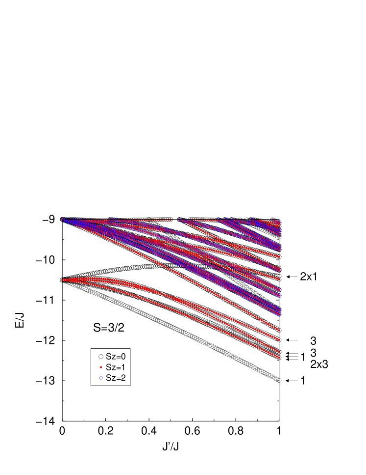
Figure 15: Spectrum of two coupled triangles in the kagomé geometry with $S=3/2$ spins. The 16 states targeted by the CORE algorithm are indicated by the arrows and their degeneracies.

Based on the two-triangle spectra shown above we used the CORE algorithm to determine the coefficients of the general two-body Hamiltonian [Eqn. (III.2)]. For an independent derivation, see Ref. [Auerbach_Kagome, ]. The coefficients obtained this way are shown in Figs. 16 and 17 for $S=1/2$ and $S=3/2$ respectively.

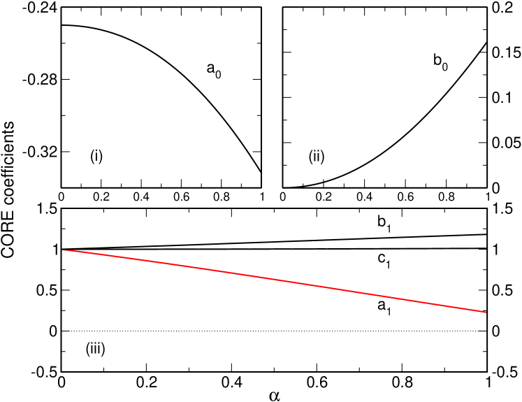
Figure 16: Coefficients of the CORE range-two Hamiltonian for two coupled $S=1/2$ triangles. The coefficients in panel (iii) have been divided by their values in the perturbative limit.

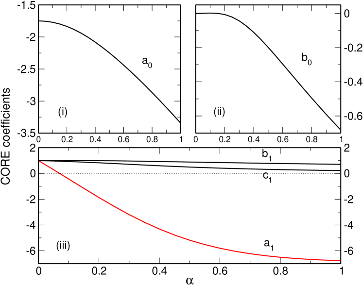
Figure 17: Coefficients of the CORE range-two Hamiltonian for two coupled $S=3/2$ triangles. The coefficients in panel (iii) have been divided by their values in the perturbative limit.

In the limit $\alpha\ll 1$ the coefficients can be obtained from the perturbative Hamiltonian [Eqn. (III.2)]. There are two classes of coefficients in both cases: $a_{0}$ and $b_{0}$ are zero in the perturbative limit, i.e. they are at least second order in $\alpha$. The second class of coefficients ($a_{1}$, $b_{1}$, $c_{1}$) are linear in $\alpha$. For improved visualisation we have divided all the coefficients in the second class by their perturbative values. In this way we observe in Fig. 16 that coefficients $b_{1}$ and $c_{1}$ change barely with respect to their values in the perturbative limit. However $a_{1}$ has a significant subleading contribution, which leads to a rather large reduction upon reaching the $\alpha=1$ point. It does however not change sign.

The situation for the $S=3/2$ case in Fig. 17 is different: while the coefficients $b_{1}$ and $c_{1}$ decrease somewhat, it is mainly $a_{1}$ which changes drastically as we increase $\alpha$. Starting from 1 it rapidly goes through zero ($\alpha\approx 0.07$) and levels off to roughly -7 times the value predicted by perturbation theory as one approaches $\alpha=1$. In this case it is rather obvious that this coefficient will dominate the effective Hamiltonian. We will discuss the implications of this behavior in the application to the $S=3/2$ kagomé magnet below.

Let us note that the behavior of the $a_{1}$ coefficient is mainly due to a rather large second order correction in perturbation theory. Indeed we find good agreement with the values obtained in the perturbative approach of Ref. [Raghu, ].

III.2.2 Simulations for $S=1/2$

After having studied the CORE basis and the effective Hamiltonian at range two in some detail, we now proceed to the actual simulations of the resulting model. We perform the simulations for the standard kagomé lattice, therefore $\alpha=1$. We will calculate several distinct physical properties, such as the tower of excitations, the evolution of the triplet gap as a function of system size and the scaling of the number of singlets in the gap. These quantities have been discussed in great detail in previous studies of the kagomé $S=1/2$ antiferromagnet LeungElser ; Lecheminant ; Waldtmann ; MilaPRL ; MambriniMila .

First we calculate the tower of excitations for a kagomé $S=1/2$ system on a 27 sites sample. The data is plotted in Fig. 18. The structure of the spectrum follows the exact data of Ref. [Lecheminant, ] rather closely; i.e there is no QDJS ensemble visible, a large number of $S=1/2$ states covering all momenta are found below the first $S=3/2$ excitations and the spectrum is roughly bounded from below by a straight line in $S(S+1)$. Note that the tower of states we obtain here is strikingly different from the one obtained in the Néel ordered square lattice case, see Fig. 11.

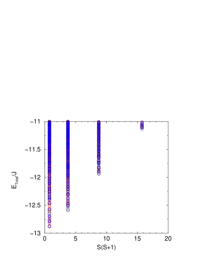
Figure 18: Tower of states obtained with a range-two CORE Hamiltonian on an effective $N=27$ kagomé lattice (9-site CORE cluster). There is a large number of low-lying states in each $S$ sector. The symbols correspond to different momenta.

Next we calculate the spin gap using the range-two CORE Hamiltonian. Results for system sizes up to 48 sites are shown in Fig. 19, together with ED data where available. In comparison we note two observations: (a) the CORE range-two approximation seems to systematically overestimate the gap, but captures correctly the sample to sample variations. (b) the gaps of the smallest samples (effective $N$=12,15) deviate strongly from the exact data. We observed this to be a general feature of very small clusters in the CORE approach. In order to improve the agreement with the ED data we calculated the two CORE range-three terms containing a closed loop of triangles. The results obtained with this extended Hamiltonian are shown as well in Fig. 19. These additional terms improve the gap data somewhat. We now find the CORE gaps to be mostly smaller than the exact ones. The precision of the CORE gap data is not accurate enough to make a reasonable prediction on the spin gap in the thermodynamic limit. However we think that the CORE data is compatible with a finite spin gap.

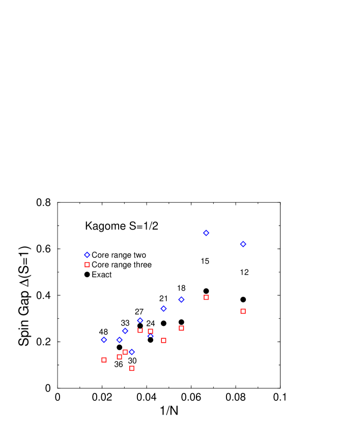
Figure 19: Spin gap of the kagomé $S=1/2$ model on various samples, obtained with the CORE method (range-two and three). Exact diagonalization result are also shown for comparison where available.

Finally we determine the number of nonmagnetic excitations within the magnetic gap for a variety of system sizes up to 39 sites. Similar studies of this quantity in ED gave evidence for an exponentially increasing number of singlets in the gap Lecheminant ; Waldtmann . We display our data in comparison to the exact results in Fig. 20. While the precise numbers are not expected to be recovered, the general trend is well described with the CORE results. For both even and odd $N$ samples we see an exponential increase of the number of these nonmagnetic states. In the case of $N=39$ for example, we find 506 states below the first magnetic excitation. These results emphasize again the validity of the two doublet basis for the CORE approach on the kagomé spin 1/2 system.

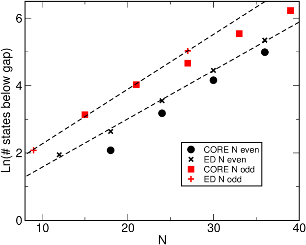
Figure 20: Logarithm of the number of states within the magnetic gap. Results obtained with the CORE range-two Hamiltonian. For comparison exact data obtained in Refs. [Lecheminant, ,Waldtmann, ] are shown. The dashed lines are linear fits to the exact diagonalization data.

III.2.3 Simulations for $S=3/2$

We have also simulated the CORE Hamiltonian obtained above for $S=3/2$. While the energy per site is reproduced roughly, unfortunately the spectrum does not resemble an antiferromagnetic spin model, i.e. the groundstate is polarized in the spin variables. This fact is at odds with preliminary exact diagonalization data on the original $S=3/2$ model KagThreeHalf . We therefore did not pursue the CORE study with this choice of the basis states any further. Indeed, as suggested by the analysis of the density matrix and by the evolution of the spectrum of two coupled triangles, we consider this a breakdown example of a naive range-two CORE approximation. It is important to stress that the method indicates its failure in various quantities throughout the algorithm, therefore offering the possibility of detecting a possible breakdown.

As a remedy in the present case we have extended the basis states to include all the $S=1/2$ and $S=3/2$ states on a triangle (i.e. keeping 20 out of 64 states). Computations within this basis set are more demanding, but give a better agreement with the exact diagonalization results. At the present stage we cannot decide whether the breakdown of the 4 states CORE basis is related only the CORE method or whether it implies that the kagomé $S=1/2$ and $S=3/2$ systems do not belong to the same phase.

IV Conclusions

We have discussed extensively the use of a novel numerical technique - the so-called numerical Contractor Renormalization (CORE) method - in the context of low-dimensional quantum magnetism. This method consists of two steps: (i) building an effective Hamiltonian acting on the low-energy degrees of freedom of some elementary block; and (ii) studying this new model numerically on finite-size clusters, using a standard Exact Diagonalization or similar approach.

Like in other real-space renormalization techniques the effective model usually contains longer range interactions. The numerical CORE procedure will be most efficient provided the effective interactions decay sufficiently fast. We discussed the validity of this assumption in several cases.

For ladder type geometries, we explicitely checked the accuracy of the effective models by increasing the range of the effective interactions until reaching convergence. Both in the perturbative regime and in the isotropic case, our results on a 2-leg ladder and a 3-leg torus are in good agreement with previously established results. This rapid convergence might be due to the small correlation length that exists in these systems which both have a finite spin gap.

In two dimensions, we have used the density matrix as a tool to check whether the restricted basis gives a good enough representation of the exact states. When this is the case, as for the plaquette lattice or the $S=1/2$ kagomé lattice, the lowest order range-two effective Hamiltonian gives semi-quantitative results, even away from any perturbative regime. For example we can successfully describe the plaquette lattice, starting from the decoupled plaquette limit through the quantum phase transition to the Néel ordered state at homogeneous coupling. Furthermore we can also reproduce many aspects of the exotic low-energy physics of the $S=1/2$ kagomé lattice.

Therefore within the CORE method, we can have both the advantage of working in a strongly reduced subspace and not being limited to the perturbative regime in certain cases.

We thus believe that the numerical CORE method can be used systematically to explore possible ways of generating low-energy effective Hamiltonians. An important field is for example the doped frustrated magnetic systems, where it is not easy to decide which states are important in a low-energy description, and therefore the density matrix might be a helpful tool.

Appendix A Density Matrix

In this appendix we introduce the density matrix of a basic building block in a larger cluster of the fully interacting problem as a diagnostic tool to validate or invalidate a particular choice of retained states on the basic building block in the CORE approach.

In previous applications of the CORE method, the choice of the states kept relied mostly on the spectrum of an isolated building block. While this usually gives reasonable results it is not a clear a priori where to place the cut-off in the spectrum.

The density matrix of a “system block” embedded in a larger “super block” forms a key concept in the Density Matrix Renormalization Group (DMRG) algorithm invented by S.R. White in 1992 DMRG and is at the heart of its success. Based on this and related ideas DMPhonons we propose to monitor the density matrix of the basic building block embedded in a larger cluster and to retain these states exhausting a large fraction of the density matrix weight.

Consider now a subsystem $\mathcal{A}$ embedded in a larger system $\mathcal{B}$. Suppose that the overall system $\mathcal{B}$ is in state $|\Psi\rangle$ (e.g. the groundstate). We write the wavefunction as:

$$|\Psi\rangle=\sum_{a,b}\ \psi_{a,b}\ |a\rangle\otimes|b\rangle,$$ (9)

where the sum index $a$ runs over all states in $\mathcal{A}$ and index $b$ over all states in $\mathcal{B}\setminus\mathcal{A}$. The density matrix $\rho^{\mathcal{A}}$ of the subsystem $\mathcal{A}$ is then defined as

$$\rho^{\mathcal{A}}_{a,a^{\prime}}=\sum_{b}\psi_{a,b}\psi_{a^{\prime},b}^{*}$$ (10)

The eigenvalues of $\rho^{\mathcal{A}}$ denote the probability of finding a certain state $a$ in $\mathcal{A}$, given the overall system in state $|\Psi\rangle$.

Practically we calculate the groundstate of the fully interacting system on a medium size cluster by exact diagonalization, and then obtain the density matrix of a basic building block, e.g. a four site plaquette. The density matrix of a building block is a rather local object, so we expect that results on intermediate size clusters are already accurate on the percent level. The density matrix spectra shown in Figs. 8 and 13 have been obtained in this way. In the models considered, a density matrix weight of the retained states of at least 90% yielded reasonable results within a range-two CORE approximation. It is possible to allow for a lower overall weight, at the expense of increasing the range of the CORE interactions.

Appendix B Observables in the numerical CORE method

The calculation of observables beyond simple energy related quantities is not straightforward within the CORE method, as the observables need to be renormalized like the Hamiltonian in the first place core-bosonfermion ; dynamicCORE .

A somewhat simpler approach for measurements of symmetry breaking order parameters consists in adding a small symmetry breaking field to the Hamiltonian (for a review see Ref. [capriotti, ]).

Let us denote ${\cal\hat{O}}$ the extensive symmetry breaking operator, such that the order parameter is related to its GS average value $m=1/N\langle\psi_{0}|{\cal\hat{O}}|\psi_{0}\rangle$. The occurence of a symmetry broken phase can be detected by adding this operator to the Hamiltonian :

$${\cal H}(\delta)={\cal H}-\delta{\cal\hat{O}}$$ (11)

Since on a finite-size lattice the order parameter vanishes by symmetry for $\delta=0$, the ground-state energy per site varies quadratically for small $\delta$ :

$$e(\delta)\simeq e_{0}-\frac{1}{2}\chi_{0}\delta^{2},$$

where $\chi_{0}$ is termed the corresponding generalized susceptibility. In that way the second derivative of the energy with respect to $\delta$ at $\delta=0$ offers one possibility to detect a finite order parameter in the thermodynamic limit capriotti .

We found that another possibility to conveniently track the presence of a finite order parameter is to measure directly $m(\delta)$ in finite field

$$m(\delta)=\langle\Psi_{\delta}|{\cal\hat{O}}|\Psi_{\delta}\rangle=\mbox{d}e(\delta)/\mbox{d}\delta$$

by the Hellmann-Feynman theorem. When plotting $m(\delta)$ as a function of the rescaled field $N\delta$ for various system sizes we observe an approximate crossing of the curves if there is a finite order parameter and no crossing in the absence of the order parameter.

Appendix C Gauge invariance on half-integer spins kagomé like systems

In this appendix, we discuss half-integer spin Hamiltonians with triangles as the unit cell. The ground state manifold of each unit cell is generated by the four degenerate lowest states that can be built out of $3$ half-integer $S$ spins, namely the four $S_{\rm tot}=1/2$ states. The idea of selecting these states as a starting point to describe the whole system low energy properties was originally introduced by Subrahmanyam for $S=1/2\$ Subrahmanyam on the kagomé lattice and later used by Mila MilaPRL . More recently it was reintroduced by Raghu et al Raghu for arbitrary half-integer $S$ in the context of a chain of triangles. All these approaches are pertubative and state that the triangle couplings $J$ is much larger than the inter-triangle one $J^{\prime}$.

Here we would like to discuss some general properties of any effective Hamiltonian that can be derived either by perturbative methods or more sophisticated ones such as CORE. In particular, we would like to point out that a gauge invariance appears as a direct consequence of the state selection.

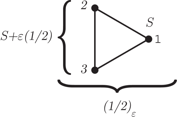
Figure 21: Definition of chirality $\varepsilon$ (see text for details).

To be more specific, let us label $1$,$2$,$3$ the sites of the triangle (see Fig. 21). In order to build a total spin $1/2$ out of the three $S$, spins $2$ and $3$ couple into a $S+\varepsilon(1/2)$ with $\varepsilon=\pm 1$. The coupling with the remaining site $1$ produces a spin $1/2$ with chirality $\varepsilon=\pm 1$. Note that this definition of chirality is equivalent to Eqs. (4) for spin $S=1/2$ up to a global unitary transform which is just a redefinition of the chirality quantification axis.

In the following, the four selected spin-chirality states on a triangle $i$ will be denoted as $||\varepsilon_{i},\nu_{i}\rangle\rangle$. These states are the eigenstates of the $z$ components of spin $\vec{\sigma}$ and chirality $\vec{\tau}$ (both are spin 1/2 like operators) with $\tau_{z}||\varepsilon_{i},\nu_{i}\rangle\rangle=(\varepsilon_{i}/2)||\varepsilon_{i},\nu_{i}\rangle\rangle$ and $\sigma_{z}||\varepsilon_{i},\nu_{i}\rangle\rangle=\nu_{i}||\varepsilon_{i},\nu_{i}\rangle\rangle$.

Let us now turn to the two-triangle problem. As it can be seen in Fig. 22, the Hamiltonian is invariant under reflections with respect to the $(xx^{\prime})$ axis. Moreover, the reflection can be taken independently on each triangle. As a consequence, both chiralities ($\tau_{i}^{z}$ and $\tau_{j}^{z}$) are conserved by the effective Hamiltonian and the $\tau$ part is of the form $1+a(\tau_{i}^{z}+\tau_{j}^{z})+b\tau_{i}^{z}\tau_{j}^{z}$. For any fixed value of $(\varepsilon_{i},\varepsilon_{j})$, the total spin of the system is conserved and thus the spin part is $SU(2)$ invariant. As a conclusion the most general two-triangle Hamiltonian allowed is of the form:

$$(\vec{\sigma}_{i}\cdot\vec{\sigma}_{j}+c)(1+a(\tau_{i}^{z}+\tau_{j}^{z})+b\tau_{i}^{z}\tau_{j}^{z}).$$

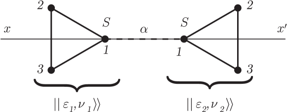
Figure 22: The two-triangle problem. $\alpha$ is the coupling ratio $J^{\prime}/J$.

Gauge transformation: The form of the above Hamiltonian is the consequence of the particular choice we made for labeling the sites of the triangle (see Fig. 22): site $1$ of triangle $t_{1}$ couples to site $1$ of triangle $t_{2}$. Although this gauge was convenient for the calculation, in general this choice can not be made simultaneously on all couples of triangles of the lattice. So, it is essential to derive the form of the Hamiltonian in a generic situation where site $i=1,2,3$ of triangle $t_{1}$ couples to site $j=1,2,3$ of triangle $t_{2}$.

The unitary transformations involved in the redefinition of the coupling sequence (see Fig. 23) are covered by the $3j$ symbols of elementary quantum mechanics. The problem of 3 half-integer spins $S$ coupled into a total spin $1/2$ occurs to be particularly simple and independent of $S$. The form of the general effective Hamiltonian then reads:

$${\cal H}_{ij}^{a,b}(\alpha) = \left(\vec{\sigma}_{i}\cdot\vec{\sigma}_{j}+c(\alpha)\right)$$

$$\times[1+a(\alpha)(\vec{\tau}_{i}\cdot\vec{e}_{a}+\vec{\tau}_{j}\cdot\vec{e}_{b})$$

$$\quad+b(\alpha)(\vec{\tau}_{i}\cdot\vec{e}_{a})(\vec{\tau}_{j}\cdot\vec{e}_{b})],$$

where $\vec{e}_{a}$, $a=1,2,3$ are three coplanar normalized vectors in a $120^{\circ}$ configuration (for example, $\vec{e}_{1}=(0,1)$, $\vec{e}_{2}=(-\sqrt{3}/2,-1/2)$ and $\vec{e}_{3}=(\sqrt{3}/2,-1/2)$ in the $x-z$ plane) and $a$, $b$ are the labels of the original spins coupling triangles $t_{i}$ and $t_{j}$.

The kagomé lattice: In the particular geometry of the kagomé lattice [see Fig. 7 (b)], each triangular unit cell is coupled to six other triangular cells, each corner being coupled twice. As a consequence, for each cell the contribution involving only $\vec{\tau}_{i}\cdot\vec{e}_{\alpha}$ factorizes into $2\vec{\tau}_{i}\cdot(\vec{e}_{1}+\vec{e}_{2}+\vec{e}_{3})=0$. The corresponding terms are then not relevant in the Hamiltonian and thus we denote the most general two-triangle Hamiltonian for the kagomé lattice as:

$${\cal H}^{=}Na_{0}(\alpha)+\sum_{\langle i,j\rangle} [b_{0}(\alpha)\vec{\tau}_{i}\cdot\vec{e}_{ij}\vec{\tau}_{j}\cdot\vec{e}_{ij}$$

$$+a_{1}(\alpha)\vec{\sigma}_{i}\cdot\vec{\sigma}_{j}$$

$$+b_{1}(\alpha)\vec{\sigma}_{i}\cdot\vec{\sigma}_{j}(\vec{\tau}_{i}\cdot\vec{e}_{ij})(\vec{\tau}_{j}\cdot\vec{e}_{ij})$$

$$+c_{1}(\alpha)\vec{\sigma}_{i}\cdot\vec{\sigma}_{j}(\vec{\tau}_{i}\cdot\vec{e}_{ij})+(\vec{\tau}_{j}\cdot\vec{e}_{ij})]$$

which is the form used in the text.

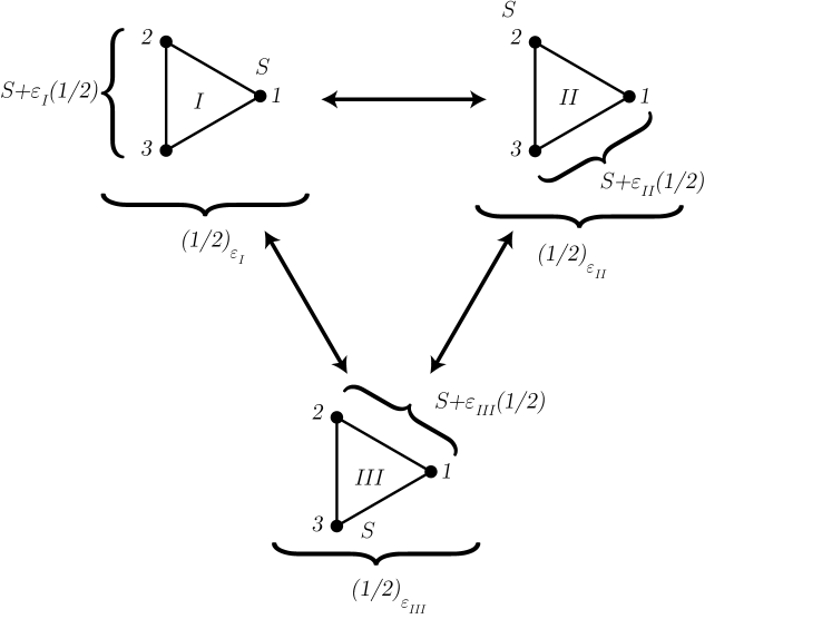
Figure 23: Three ways of coupling the three spins $S$ on a triangle into a total spin $1/2$ state. Each construction is related to the two others by the 3$j$ symbols (see text).

References

- (1) C.J. Morningstar and M. Weinstein, Phys. Rev. Lett. 73, 1873 (1994); C.J. Morningstar and M. Weinstein, Phys. Rev. D 54 4131 (1996).
- (2) M. Weinstein, Phys. Rev. B 63 174421 (2001).
- (3) E. Altman and A. Auerbach, Phys. Rev. B 65, 104508 (2002).
- (4) E. Berg, E. Altman, and A. Auerbach, Phys. Rev. Lett. 90, 147204 (2003).
- (5) J. Piekarewicz and J.R. Shepard, Phys. Rev. B 56, 5366 (1997).
- (6) J. Piekarewicz and J.R. Shepard, Phys. Rev. B 57, 10260 (1998).
- (7) S. Capponi and D. Poilblanc, Phys. Rev. B 66, 180503(R) (2002).
- (8) J.-P. Malrieu and N. Guihéry, Phys. Rev. B 63, 085110 (2001).
- (9) E. Dagotto and T. M. Rice, Science 271, 618 (1996) and references therein.
- (10) T. Barnes, E. Dagotto, J. Riera, and E. S. Swanson, Phys. Rev. B 47, 3196 (1993); S. R. White, R. M. Noack, and D. J. Scalapino, Phys. Rev. Lett. 73, 886 (1994); B. Frischmuth, B. Ammon, and M. Troyer, Phys. Rev. B 54, R3714 (1996).
- (11) M. Greven, R. J. Birgeneau, and U.-J. Wiese, Phys. Rev. Lett. 77, 1865 (1996).
- (12) K. Kawano and M. Takahashi, J. Phys. Soc. Jpn 66, 4001 (1997).
- (13) D.C. Cabra, A. Honecker and P. Pujol, Phys. Rev. B 58, 6241 (1998).
- (14) Proceedings of the XXXIst Rencontres de Moriond, edited by T. Martin, G. Montambaux, and J. Trân Thanh Vân, Editions Frontières, Gif-sur-Yvette, France, 1996 (cond-mat/9605075).
- (15) E. Lieb, T. Schultz, D. Mattis, Ann. Phys. 16, 407 (1961); I. Affleck, Phys. Rev. B 37, 5186 (1988).
- (16) A. Koga, S. Kumada and N. Kawakami, J. Phys. Soc. Jpn. 68, 642 (1999).
- (17) A. Koga, S. Kumada and N. Kawakami, J. Phys. Soc. Jpn. 68, 2373 (1999).
- (18) A. Läuchli, S. Wessel and M. Sigrist, Phys. Rev. B 66, 014401 (2002).
- (19) A. Voigt, Computer Physics Communication 146, 125 (2002).
- (20) P.W. Leung and V. Elser, Phys. Rev. B 47, 5459 (1993).
- (21) P. Lecheminant et al., Phys. Rev. B 56, 2521 (1997).
- (22) C. Waldtmann et al., Eur. Phys. J. B 2, 501 (1998).
- (23) F. Mila, Phys. Rev. Lett. 81, 2356, (1998).
- (24) M. Mambrini and F. Mila, Eur. Phys. J. B 17, 651 (2000).
- (25) V. Subrahmanyam, Phys. Rev. B 52, 1133 (1995).
- (26) C. Raghu, I. Rudra, S. Ramasesha and D. Sen, Phys. Rev. B 62, 9484 (2000).
- (27) B. Bernu, C. Lhuillier, and L. Pierre, Phys. Rev. Lett. 69, 2590 (1992).
- (28) P. Sindzingre, C. Lhuillier, J.B. Fouet, Int. J. Mod. Phys B 17 5031 (2003); (cond-mat/0110283).
- (29) M. Calandra and S. Sorella, Phys. Rev. B 61, R11894 (2000).
- (30) L. Capriotti, Int. J. Mod. Phys. B 15, 1799 (2001).
- (31) L. Limot, P. Mendels, G. Collin, C. Mondelli, B. Ouladdiaf, H. Mutka, N. Blanchard, and M. Mekata, Phys. Rev. B 65, 144447 (2002), and references therein.
- (32) R. Budnik and A. Auerbach, unpublished; R. Budnik, M.Sc. thesis (Technion, Haifa).
- (33) S. Dommange, A. Läuchli, J.-B. Fouet, B. Normand and F. Mila, unpublished.
- (34) S.R. White, Phys. Rev. Lett. 69, 2863 (1992).
- (35) C. Zhang, E. Jeckelmann, and S.R. White, Phys. Rev. Lett. 80, 2661 (1998).