An empirical test for cellular automaton models of traffic flow

Abstract

Based on a detailed microscopic test scenario motivated by recent empirical studies of single-vehicle data, several cellular automaton models for traffic flow are compared. We find three levels of agreement with the empirical data: 1) models that do not reproduce even qualitatively the most important empirical observations, 2) models that are on a macroscopic level in reasonable agreement with the empirics, and 3) models that reproduce the empirical data on a microscopic level as well. Our results are not only relevant for applications, but also shed new light on the relevant interactions in traffic flow.

]

I Introduction

For a long time the modeling of traffic flow phenomena was dominated by two theoretical approaches (for a review, see e.g., [1, 2, 3, 4]). The first type of models, the so-called car-following models, are based on the fact that the behavior of a driver is determined by the leading vehicle. This assumption leads to dynamical velocity equations which in general depend on the distance to the leading vehicles and on the velocity difference between the leading and the following vehicle. An alternative approach, which is also well established in traffic research, does not treat the individual cars but describes the dynamics of traffic networks in terms of macroscopic variables. Here traffic flow phenomena are treated in analogy to the dynamics of compressible viscous fluids.

Both approaches are still widely used by traffic engineers, but for practical purposes they are often not suitable. One of the main problems of present car-following models (e.g., see [5, 6, 7, 8, 9]) is that they are difficult to treat in computer simulations of large networks. On the other hand also the macroscopic approaches lead to some difficulties although large networks can be treated in principle. First of all, present macroscopic models use a large number of parameters which have partly no counterpart within empirical investigations. In addition to that, the information that can be obtained using macroscopic models is incomplete in the sense that it is not possible to trace individual cars.

In order to fill this gap cellular automaton (CA) models have been invented [10, 11]. CA models are microscopic models which are by design well suited for large-scale computer simulations. A comparison of the simulations with empirical data shows that already very simple approaches give meaningful results. In particular they can be used in order to simulate dense networks like cities [12] which are controlled by the dynamics at the intersections. For highway traffic, however, a more detailed description of the dynamics seems to be necessary.

In this work we want to discuss the realism and the limitations of a number of CA models. Our choice is restricted to models that are discrete in space and time, which e.g. excludes the approach by Krauss et al. [13], and have local interactions only, excluding models as the Galilei-invariant model introduced in [14]. We compare simulations of the CA model proposed by Nagel and Schreckenberg, that is to date the most frequently used CA approach for traffic flow, the VDR model [15] which realizes a so-called slow-to-start rule, the TOCA-model of Brilon et al. [16], the model of Emmerich and Rank [17] based on the use of velocity-gap matrices, and the approach by Helbing and Schreckenberg [18] which represents a model with a more sophisticated distance rule. Finally we discuss the recently introduced brake light model [19, 20] that was suggested in order to give a reliable reproduction of the microscopic empirics and the model by Kerner, Klenov and Wolf [21], focusing more on the macroscopic properties of the three phases of traffic flow.

We will compare the ability of these models to reproduce the empirical findings. This requires using a measurement procedure in the simulations which models the detectors on the highway. Analogous to the empirical setup of [22] the simulation data are evaluated by a virtual inductive loop, i.e., speed and time-headway of the vehicles are measured at a given link of the lattice. The measurement process is applied after the update of the velocity has been carried out, but right before the movement of the vehicles. This implies that the gap to the preceding vehicle does not change significantly during the measurement. These simulation data are analyzed regarding individual and aggregated quantities, as it has been done in recent empirical investigations [22, 23, 24].

Although most of the empirical data sets have been collected at multi-lane highways, we have performed our simulations on a single-lane road in order to reduce the number of adjustable parameters. This approach is justified because the empirical data sets are selected such that multi-lane effects are of minor importance. They might play a role for synchronized traffic of type $(i)$ and $(ii)$, as it has been recently argued in [25], but in any case these types of synchronized traffic are much rarely observed than synchronized traffic of type $(iii)$ [22, 24].

We will also not consider effects by a mixture of different vehicle types, e.g. there are no trucks in our simulations. The fraction of slow cars has not been determined from the empirical data. Furthermore these data have been collected on a highway with speed limit such that disorder effects through slower cars are expected to play a minor role. We believe that inclusion of disorder will not change our results qualitatively, but can lead to a better quantitative agreement in some cases.

Before we start the analysis of the above mentioned CA models, we will introduce an empirical test scenario. It will be microscopic and local to make it easily comparable to online data provided e.g. by inductive loops. In contrast, the detection of complex spatio-temporal structures [26] is more difficult to achieve in an automated way. It would require the investigation of interface dynamics whereas in our scenario only bulk properties are studied. This test scenario also verifies the reproduction of empirical traffic states on a microscopic level, a task that cannot be fulfilled by macroscopic models. The empirical results have been chosen with respect to their reproducibility and the ability to distinguish between the different states of traffic. This scenario will be discussed in the next section.

II Empirical facts

In order to probe the accuracy and the degree of realism of the different models one has to introduce a test scenario that includes the most important empirical findings. The difficulty in defining such a scenario is due to the fact that the empirical results may depend strongly on the particular environment. Therefore one has to try to extract the results that really characterize the behavior of the vehicles. As an additional difficulty mostly aggregated data have been analyzed which are known to be largely dependent on the road conditions, e.g., the capacity of an upstream bottleneck. A number of results, however, is of general nature as we will discuss below.

Even more conclusive are empirical investigations that use single-vehicle data. These measurements can be compared directly to the simulation results and include important information concerning the microscopic structure of vehicular traffic. Unfortunately only a small number of empirical investigations based on single-vehicle data exists so far. Our discussion refers to the empirical studies of refs. [22, 23, 24]. In particular, in order to reduce the effects of disorder, the results of [22] (except for the time-headway distributions, see below) are used for the comparison with simulation data. These data have been collected on a highway where a speed limit applies. This facilitates the comparison with modeling approaches.

The empirical findings that are taken as a basis for the comparison with the model results have been obtained from inductive loops. Measurements by inductive loops, which represent the most frequently used measurement devices, give information about the number of cars passing, their velocities and the occupation times. These direct measurements are also used in order to calculate other quantities, e.g., the spatial distance $d_{n}$ via $d_{n}=v_{n-1}t_{h}$ (where $v_{n-1}$ denotes the velocity of the preceding car ${n-1}$, $t_{h}$ the time-headway between car $n-1$ and car $n$).

A Temporally aggregated data

The most important empirical quantity is the relation between the averaged observables flow and density, i.e., the fundamental diagram. There exists a longstanding controversy (see e.g. [26, 27] and references therein) about the “correct” functional form of the fundamental diagram and a large number of possible forms have been suggested to be compatible with empirical data [28]. A more consistent picture was established after the work of Kerner and coworkers who distinguished at least three different phases of traffic flow [29], i.e., free flow, synchronized traffic and wide jams, that have to be analyzed separately. We will follow this scheme and summarize the empirical findings accordingly.

Usually these measurements are stored as averaged values of certain time-intervals. We discuss results for the fundamental diagram, i.e., the flow density relation, in the different traffic phases that are based on one-minute data. The results for the functional form of the flow are shown, as far as possible, in dependence of the spatial density $\rho(t)$. The density can be calculated from

$$\rho(t)=\frac{J(t)}{v(t)},$$ (1)

where $J(t)$ denotes the number of cars passing the detector with an average velocity $v(t)$ in the corresponding time interval.

Free flow traffic is characterized by a large value of the average speed. One basically observes two qualitatively different functional forms of the fundamental diagram, i.e., that the linear regime extends up to the observed maximum of the flow or that one has a finite curvature in particular for densities slightly below the density of maximum flow [24, 30]. The finite curvature is a consequence of an alignment of speeds, i.e., close to the optimal flow it is not longer possible to drive systematically faster than the trucks. This point of view is supported by the empirical results taken from highways where a quite restrictive speed limit is applied that can be reached even by trucks [22].

In this case the whole free flow branch is linear. For our purposes the linear form of the fundamental diagram is relevant, because we use a single type of cars in the simulations, with a maximal velocity that is given by the slope of the free flow branch. When simulating a section of the highway where no speed limit is applied, one has to take a distribution of maximal speeds. This distribution can be obtained from the empirical velocity distributions at very low densities, where interactions between cars can be neglected.

In the congested regime one distinguishes between synchronized traffic and wide jams. In the synchronized phase, the mean velocity of the vehicles is reduced, compared to the free flow, but the flow can take on values close to the maximum flow. Moreover, strong correlations between the density on different lanes exist caused by lane changings.

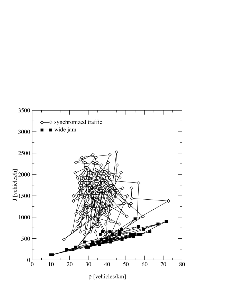
FIG. 1.: Time-traced fundamental diagram of the two congested states (from [30]). Synchronized traffic is characterized by strong fluctuations of the density and flow. The measurements for wide jams are similar to measurements in free flow but with much smaller average velocity.

The synchronized state has been subdivided into three types, which differ in the characteristics of the time series of density and flow: In synchronized traffic of type $(i)$ constant values of the density and the flow can be observed during a long period of time. In synchronized traffic of type $(ii)$ the flow depends linearly on the density similarly to free flow, but the mean velocity is reduced considerably. In synchronized traffic of type $(iii)$ irregular patterns of flow and density can be observed (Fig. 1). In our article we concentrate on synchronized flow of type $(iii)$, because the two other types of synchronized traffic have been rarely observed and it is not confirmed whether they are generic phases of traffic flow. An identification of synchronized traffic by means of the fundamental diagram may be misleading, because the results often depend on the averaging procedure. A more sensitive check is to identify the different types of traffic states by means of the cross-correlation $cc(\rho,J)$ of the density $\rho$ and the flow $J$ [22]:

$$cc(\rho,J)=\frac{\langle\rho(t)J(t+\tau)\rangle-\langle\rho(t)\rangle\langle J(t+\tau)\rangle}{\sqrt{\Delta\rho(t)}\ \sqrt{\Delta J(t+\tau)}}$$ (2)

with $\Delta A=\langle A^{2}\rangle-\langle A\rangle^{2}$ denoting the variance of the observable $A$. The linear dependency of the flow and the density in the free flow state as well as in the wide jam state leads to cross-correlations of $\approx 1$, whereas irregular patterns of the flow and the density in the synchronized traffic of type $(iii)$ lead to cross-correlations of $\approx 0$.

It is worth pointing out that the notion of “synchronized traffic” is still very controversial [27, 26]. We emphasize here, that we use an objective criterion, namely the vanishing of the cross-correlation function (2) for the classification. Within the empirical single-vehicle data sets available the other two synchronized states could not be clearly identified. Therefore it was not reasonable to include these states into the test scenario. The characteristics of synchronized traffic of type $(iii)$, however, have been clearly distinguished from free flow and jammed states by the criterion $cc(\rho,J)\approx 0$. Therefore any detailed model should be able to reproduce this class of synchronized states.

Fig. 1 includes a typical measurement of the fundamental diagram that correspond to wide jams. Surprisingly these measurements reveal quite small values of the density, although the road is almost completely covered by cars. This seemingly incorrect result is due to the local nature of the measurement (see [22] for a detailed discussion). Thus, the form of the fundamental diagram in the jammed state is similar to free flow traffic, but with a small average velocity.

The jammed branch of the fundamental diagram is often not reproduced by CA models, because they use the inverse density of a jam in order to calibrate the unit of length. Within these approaches jams are compact. In this case (almost) no internal flux is observed. The modeling of jams can however be meaningful, if the upstream velocity and other macroscopic characteristics of jam are reproduced.

B Single vehicle data

Nowadays some empirical studies exist that have analyzed single-vehicle data from counting loops [22, 23, 24]. These studies are of great importance for the modeling of traffic flow because they give direct information about the “microscopic structure” of traffic streams. The data usually include direct measurements of the time-headways and the velocities of the vehicles as well as the occupation time of the detector. Similar to the time-averaged observables the results for the microscopic quantities differ qualitatively in the different phases.

The first quantity we look at is the time-headway distribution , i.e., the time elapsing between two cars passing the detector. This quantity is the microscopic analogue to the inverse flow. In free flow traffic one has found that the distribution at short times and also the position of the maximum is independent of the density (Fig. 2).

The cut-off at small time-headways as well as the typical time-headway in free flow traffic are important observables which have to be reproduced by the microscopic models. The exact shape of the distribution may also depend on the relative frequency of slow vehicles, because this determines the fraction of interacting vehicles at a given density.

The time-headway distributions in synchronized traffic  differ systematically from the free flow distributions (Fig. 3). In synchronized traffic the distributions have a maximum that is much broader than that in free flow traffic. The maximum is less pronounced and its position depends significantly on the density.

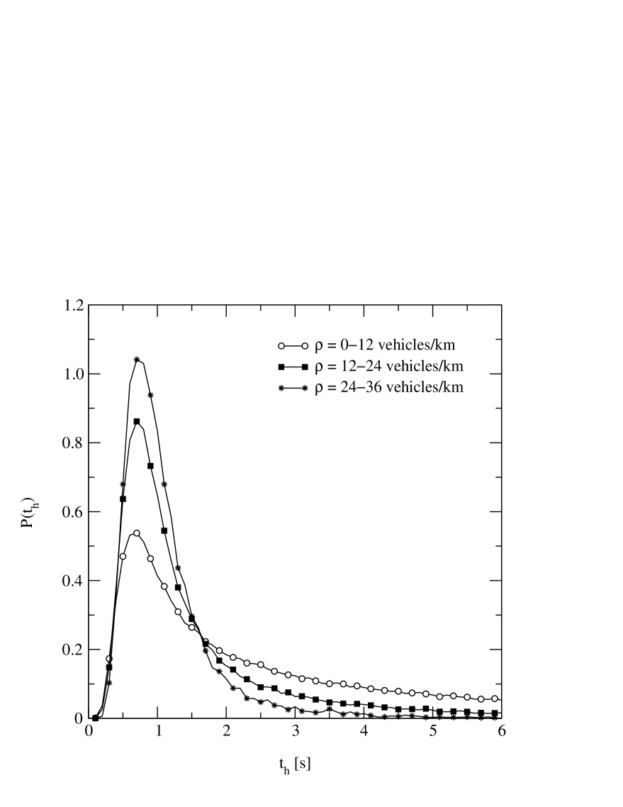
FIG. 2.: Empirical time-headway distributions, i.e., the relative frequency of a given time-headway, in free flow traffic. The distributions are normalized, i.e., $\sum P(t_{h})\cdot\Delta t_{h}=1$. The data are classified in different density regimes by the corresponding one-minute data of the density. For a given road section one obtains a maximum that is independent of the density and a minimal headway of 0.2 s.

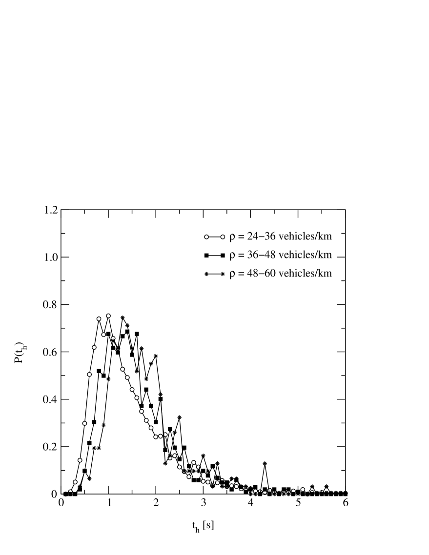
FIG. 3.: Same as Fig. 2 but for synchronized traffic. The functional behavior of the distribution at short times depends on the density.

In the presence of wide jams one has to distinguish between the jam itself and its outflow region. In the jam one finds evidently a broad distribution of time-headways, because cars are blocked for quite long times. In the outflow region of a jam, however, one observes that the typical time-headway is of the order of $\sim 2$ s.

The characteristics of traffic jams are one of the extensively studied phenomena in traffic flow. Wide traffic jams can be identified by a sharp drop of the velocity and the flow to negligible values in the time-series. Moreover traffic jams move upstream with a surprisingly constant velocity (typically $15$ km/h [31]). The upstream velocity is intimately related to the outflow $J_{\rm{out}}$ from a jam which also takes on constant values for a given situation. This allows the observed coexistence of jams. The coexistence is facilitated because the outflow from a jam is considerably smaller than the maximal flow $J_{\rm{max}}$, such that no new jams emerge in the outflow region of a jam. Empirically one observes the ratio $J_{\rm{max}}/J_{\rm{out}}\approx 1.5$ [32]. The outflow and the upstream velocity of a jam can therefore also be used to calibrate the model. The precise data for the average upstream velocities and $J_{\rm{out}}$ may also serve to evaluate the average space $l$ that is occupied by a car in a jam. Usually $l$, and not the average length of the vehicles, represents the length of a cell in the CA models. $l$ may also be used to assign a reasonable value of the velocity of cars in a jam, i.e., $v_{n}=l/t_{h}$.

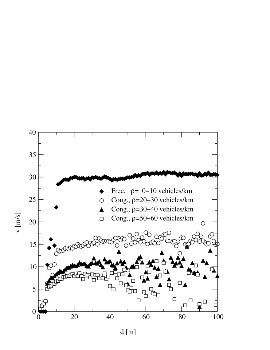
FIG. 4.: Empirical optimal-velocity (OV) functions, i.e., speed-distance relations. The figure shows the mean velocity for a given spatial distance in free flow and congested traffic for different densities.

The final test of the models comes from the velocity distance relation in the different traffic phases (Fig. 4). This relation, also called optimal-velocity (OV) function, characterizes in great detail the microscopic structure of the different phases. Some models use OV-curves directly as an input [33]. In any case this quantity is a sensitive test concerning the reproduction of the microscopic structure of highway traffic. In the free flow regime the asymptotic velocity does not depend on the density, but is given by the applied speed limit. In the congested regime this asymptotic velocity is much smaller than in free flow, i.e., cars are driving slower than the distance-headway allows. This is a direct effect of the vehicle-vehicle interactions [22] and should therefore be reproduced by any realistic traffic-model.

III Simple stochastic CA models

Throughout this article we investigate microscopic traffic models that are discrete in space and time. The discreteness of the model has the advantage of allowing direct and very efficient computer simulations, and in particular without any further discretization errors. The discreteness of the model, however, also leads to some difficulties, in particular when describing congested traffic. E.g., in congested traffic a continuous range of typical velocities exists that depend strongly on the density. This velocity interval is mapped on a discrete set of velocity variables. So even for an optimal reproduction of the traffic state an upper limit for the accuracy of the model exists. Therefore, one has to find a compromise between the degree of realism and the level of complexity by choosing an appropriate discretization of the velocity.

Moreover, the temporal discretization introduces a characteristic time-scale. This time-scale can be understood, if a parallel update is applied, as the effective reaction-time of the drivers, which is included explicitly in car-following models. Furthermore, the temporal discretization becomes obvious as peaks in the measurement of the time-headways $t_{h}$. The finer the discretization the less pronounced the peaks. In order to increase the resolution the time-headways in the simulations are calculated via the relation $t_{h}=\frac{d}{v}$ with the velocity $v$ of the vehicle and the distance-headway $d$ to the preceding vehicle. Nevertheless, the minimal resolution is restricted by the discretization that determines the minimal $t_{h}$ difference in free flow $\frac{l}{v_{\text{max}}}$ with the length $l$ and the maximum velocity $v_{\text{max}}$ of a vehicle. In order to facilitate a comparison with the empirical time-headway distribution the distributions are normalized via $\sum P(t_{h})\cdot\Delta t_{h}=1$.

Below we discuss a number of traffic models in detail and with respect to their agreement with the empirical findings of our test scenario. Beyond that we demand that each model reproduces some basic phenomena, like spontaneous jam formation, and fulfills minimal conditions as, e.g., being free of collisions. These conditions are generally understood as fulfilled, if the opposite is not explicitly stated. In particular, deterministic models (e.g. [34, 35]) are not a subject of this study. They can not reproduce the spontaneous formation of jams [11] which are the result of an inherent stochasticity of traffic flow rather than a consequence of perturbations.

Our simulations are performed on a periodic single-lane system. This simple structure of the system is in sharp contrast with realistic highway networks. It is nevertheless justified, because it has been shown for a large class of models that different boundary conditions select different steady states rather than changing their microscopic structure [36]. Therefore the boundary conditions are of great importance if one tries to reproduce the spatio-temporal structure on a macroscopic level. However, in comparison with local measurements an appropriate traffic model should be able to reproduce the empirical results also if periodic boundary conditions are applied. Furthermore the restriction to a single lane is of minor importance for the empirical test scenario which has been discussed in the previous section. In the simulations system sizes of $L\geq 10000$ cells have been used which is sufficient to reduce finite-size effects. Typical runs used 50000 time steps to reach the stationary state and measurements.

We also want to emphasize that for each model all simulations have been performed with a single set of parameters. Some of the model parameters can be directly related to a given empirical quantity. In this case we have chosen the value that leads to an optimal agreement with the related observable to avoid ranking the importance of the empirical findings. For a particular application of the model, however, the reproduction of a certain quantity might be of special interest and therefore a calibration of the model different from ours might be more appropriate.

A The CA model of Nagel and Schreckenberg

The model introduced by Nagel and Schreckenberg [10] (hereafter cited as “NaSch model”) is the prototype of microscopic models that we discuss. The important role of this model is mainly due to its simplicity which allows for very fast implementations. In fact the NaSch model is a minimal model in the sense that every further simplification leads to a loss of realism. We will also use it as a reference for other models that will be introduced by giving the relation to the NaSch model.

The NaSch model is a discrete model for traffic flow. The road is divided into cells that can be either empty or occupied by car $n$ with a velocity $v_{n}=0,1,...,v_{\text{max}}$. Cars move from the left to the right on a lane with periodic boundary conditions and the system update is performed in parallel.

For completeness we repeat the definition of the model that is given by the four following rules ($t<t_{1}<t_{2}<t+1$):

1. Acceleration: $v_{n}(t_{1})=\min\{v_{n}(t)+1,v_{\text{max}}\}$

2. Deceleration: $v_{n}(t_{2})=\min\{v_{n}(t_{1}),d_{n}(t)\}$

3. Randomization: $v_{n}(t+1)=\max\{v_{n}(t_{2})-1,0\}$ with probability $p_{\rm{dec}}$  (otherwise $v_{n}(t+1)=v_{n}(t_{2})$)

4. Motion: $x_{n}(t+1)=x_{n}(t)+v_{n}(t+1)$

with the velocity $v_{n}$, the maximum velocity $v_{\text{max}}$ and the position $x_{n}$ of car $n$. $d_{n}(t)$ specifies the number of empty cells in front of car $n$ at time $t$.

For a given discretization the model can be tuned simply by varying the two parameters $v_{\text{max}}$ and $p_{\rm{dec}}$. The value of $v_{\text{max}}$ mainly affects the slope of the fundamental diagram in the free flow regime while the behavior in the congested regime is controlled by the braking noise $p_{\rm{dec}}$. Each time-step $\Delta t$ corresponds to 1.2 s in reality in order to reproduce the empirical jam velocity at a given cell length of $7.5$ m. The length of a cell corresponds to the average space occupied by a vehicle in a jam, i.e., its length and the distance to the next vehicle ahead. This choice is in accordance with measurements at German highways on the left and middle lane, where the density of trucks is low [32]. Due to the parallel update an implicit reaction time is introduced which has to be considered when choosing the unit of time. This time is not the reaction time of the driver (that would be much shorter) but the time between the stimulus and the actual reaction of the vehicle. The value we have chosen allows to reproduce the typical upstream velocity of a jam.

We tune the two free parameters of the model by adjusting the slope in the free flow regime and the maximum of the fundamental diagram. Fig. 5 shows the resulting fundamental diagram using $v_{\text{max}}=112~{}\rm{km/h}=5~{}\rm{cells/timestep}$ and $p_{\rm{dec}}=0.16$ which has to be compared with the empirical results.

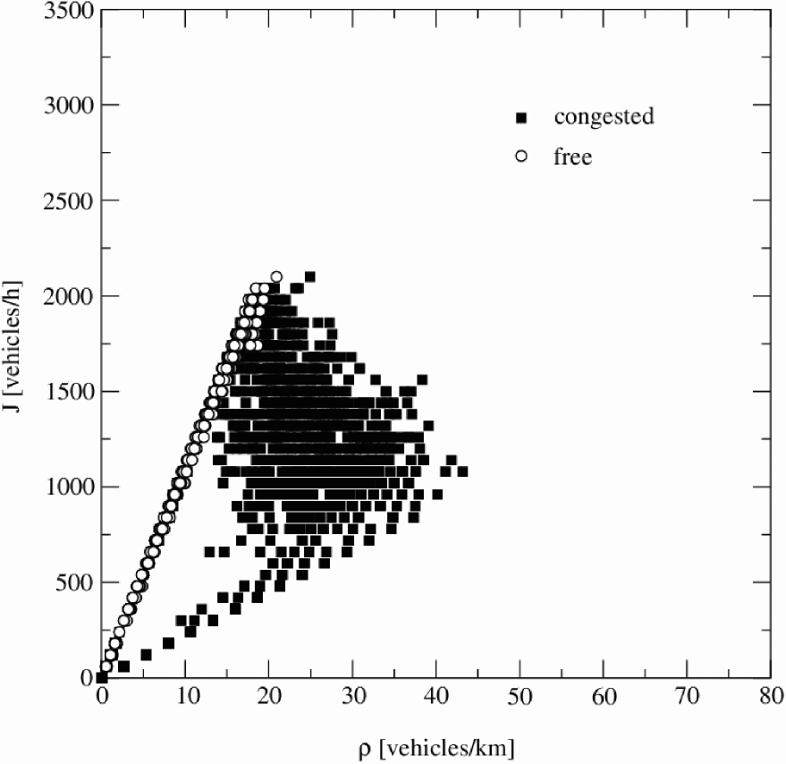
FIG. 5.: Local fundamental diagram of the NaSch model for $v_{\text{max}}=112~{}\rm{km/h}=5~{}\rm{cells}/\Delta t$, $\Delta t=1.2$ s and $p_{\rm{dec}}=0.16$. A cell has a length of $7.5$ m.

By tuning the parameters we could reproduce quite well the free flow branch of the fundamental diagram: Both, the slope as well as the maximum is in agreement with the empirical findings. For congested traffic, however, the model fails to reproduce the two distinct phases, in particular the characteristics of synchronized traffic are not matched. This interpretation of the flow data is supported by measurements of the cross-correlation function that is negative in the corresponding density regime. In the presence of wide jams the flow is proportional to the densities as found by empirical observation. But also for wide jams differences exist. In real measurements the branch extends up to quite large densities ($\sim 70$ veh/km), while the simulation results are restricted to lower densities ($\sim 40$ veh/km).

Next we discuss the model on a microscopic level. As mentioned above the upstream velocity of wide jams can be tuned by choosing the appropriate discretization $\Delta t$ of the time. We have verified our calibration by initializing the system by a large jam and measuring the velocity of the upstream propagation of the jam front. As expected our result is in agreement with the empirical data. Nevertheless the dynamics of jams in the NaSch model is in contradiction to empirical findings since its outflow from a jam equals the maximal possible flow. This implies that the observed parallel propagation of jams cannot be reproduced by the NaSch model.

The time-headway distributions of the NaSch model (see also [37]) also mismatch with empirical data (Fig. 6). Due to the discreteness of the model and the unique maximal velocity of the cars the distribution function has a peaked structure.

FIG. 6.: Normalized time-headway distribution of the NaSch model in free flow and congested traffic for different densities.

But more important than that is the absence of time-headways shorter than the chosen unit of time. This implies that we cannot reproduce the cut-off at short times and the upstream velocity of jams at the same time.

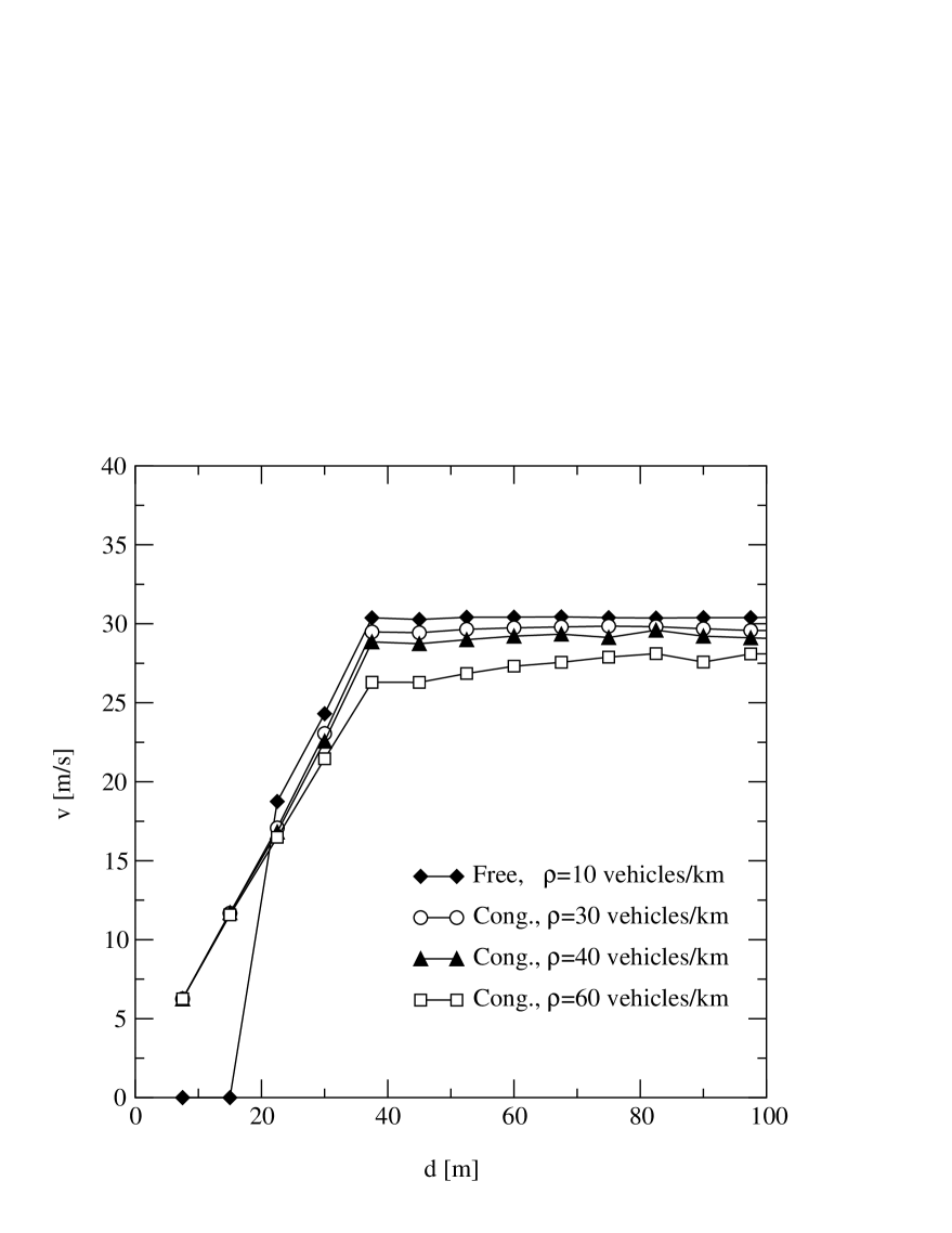
FIG. 7.: OV function in free flow and congested traffic of the NaSch model for different densities.

Finally, we also discuss the optimal velocity curves of the model (Fig. 7). In congested traffic one observes only a very weak dependence of the “optimal velocity” on the density. This is due to the short range of interactions in the model and the strong acceleration of the cars. So we neither observe a significant density dependence nor a sensitivity to the traffic state. This is a serious contradiction to the empirical findings, related to an incomplete description of the microscopic structure of the model.

B VDR model

A step towards a more realistic CA model of traffic flow was done by the so-called velocity-dependent-randomization (VDR) model [15] that extends slightly the set of update rules of the NaSch model. In this model, a velocity-dependent randomization $p_{\rm{dec}}(v)$ is introduced that is calculated before application of step 1 of the NaSch model. As simplest version, a different $p_{\rm{dec}}$ for cars with $v=0$ was studied:

$$p_{\rm{dec}}(v)=\left\{\begin{array}[]{cc}p_{0}&\ \ \text{for\ }v=0\\ p&\ \ \text{for\ }v>0\end{array}\right.$$ (3)

with $p_{0}>p$ (slow-to-start rule).

The additional rule of the VDR model has been introduced in order to reproduce hysteresis effects. This is indeed possible, because the new parameter $p_{0}$ allows to tune the velocity and outflow of wide jams separately. As a side effect it is now possible to reproduce the observed short time-headways by keeping the unit of time small and the empirical observed downstream velocity of jams. The parameters of the model were chosen in the following way: The unit of time was adjusted in order to match the position of the maximum of the time-headway distribution. Then we have chosen the parameter $p_{0}$ such that we could reproduce the measurements of the upstream velocity of a jam. Finally the values of $v_{\text{max}}$ and $p$ ensure a good agreement in the free flow branch. The behavior found in the VDR model is typical for models with slow-to-start rules [38, 39].

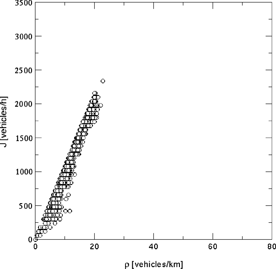
FIG. 8.: Local fundamental diagram of the VDR model for $v_{\text{max}}=108~{}\rm{km/h}=3~{}\rm{cells}/\Delta t$, $\Delta t=0.75~{}\rm{s}$, $p_{0}=0.58$ and $p=0.16$.

Fig. 8 shows the local fundamental diagram of the VDR model. For the parameter values obtained by the above procedure only very weak hysteresis effects are observed. Obviously the model fails to reproduce the empirically observed congested phase correctly. Compared to the NaSch model the mismatch of the fundamental diagram in the congested regime is even more serious, i.e., we cannot identify at all a density regime as synchronized traffic. The reason for this is a stronger separation between free flow and wide jams, which are compact. Therefore one does not observe any flow within a jam if a stationary state of a periodic system is analyzed. In case of open boundary conditions a slight broadening of the free-flow branch has been observed, if the detector is located close to the exit of the highway section. This effect is due to the smaller length scale of jams close to the exit, which leads to a larger weight of accelerating cars. Due to the coarsening of the jam size this effect vanishes in the bulk of the system [40, 41].

But in any case, this way of generating synchronized states by the boundary conditions does not agree with the empirical situation, because one cannot reproduce the large spatial and temporal extension of the synchronized state. The missing synchronized traffic phase leads to quite large positive values of the cross-correlation $cc(J,\rho)$ of the density and the flow.

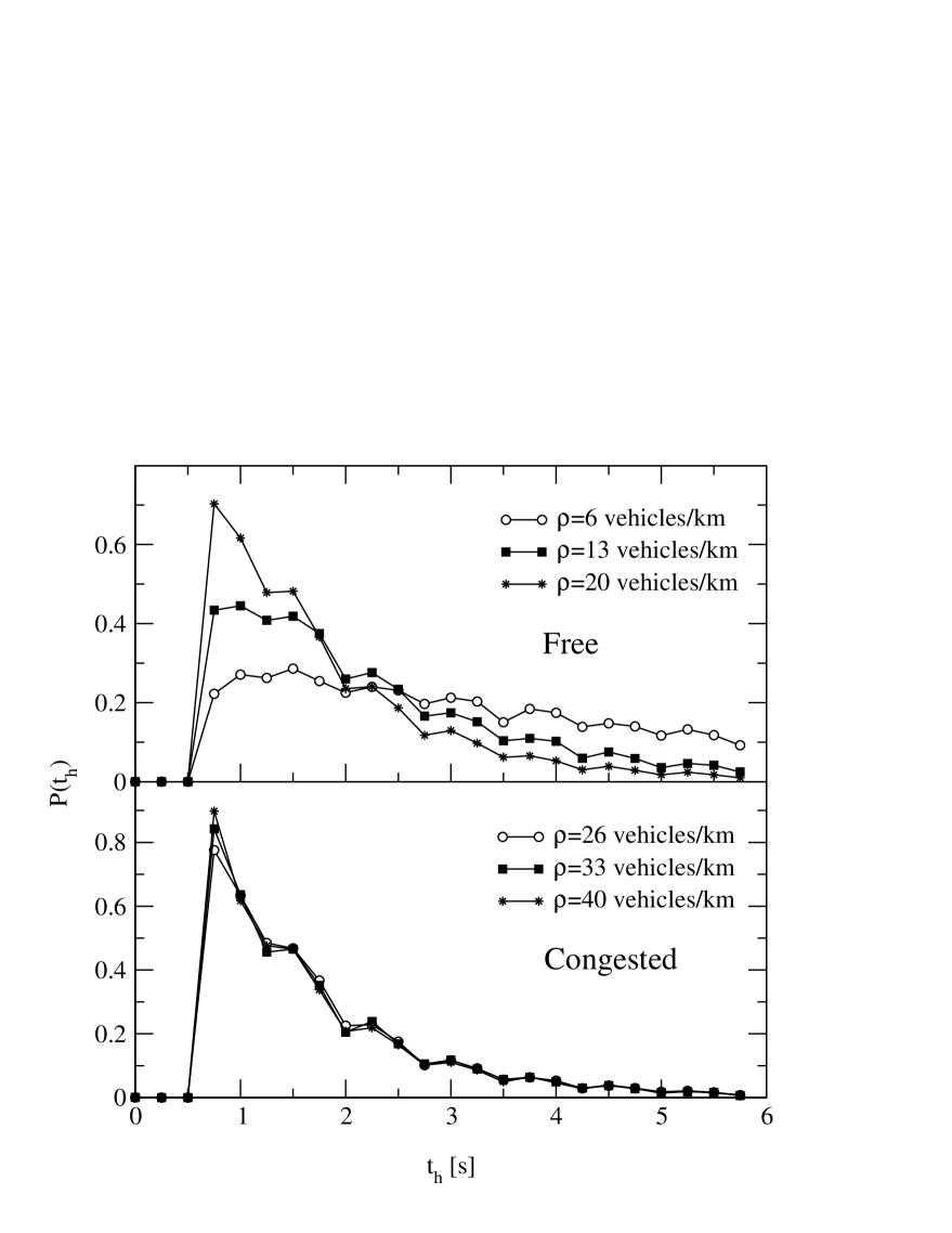
FIG. 9.: Normalized time-headway distribution of the VDR model in free flow and congested traffic for different densities.

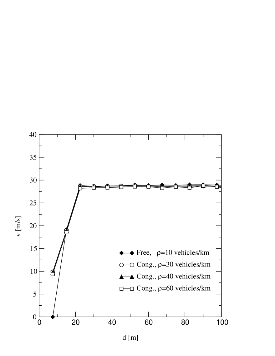
FIG. 10.: OV function of the VDR model in free flow and congested traffic for different densities.

The time-headway distribution of the VDR model differs in two points from the empirical observations (Fig. 9). (i) The unit of time is a sharp cut-off, i.e., the short time characteristics of the time-headway distribution is not in agreement with the empirical findings. (ii) We do not observe a density dependence of the maximum in congested traffic. Similar results are obtained for the OV functions, that do not depend on the density or the traffic state (Fig. 10). This result is a consequence of the microscopic structure of high density states. At large densities compact wide jams and zones of free flow traffic coexist, separated by a narrow transition layer. Now, our virtual “detector” measures only moving cars and therefore almost freely moving cars even at large densities.

The major achievement of the VDR model is the correct description of the dynamics of wide jams which is similar to the so-called local cluster effect [42] found in hydrodynamical models. The outflow from a jam is lower than the maximal flow, and therefore jams do not emerge in the outflow region. This effect leads to the increased stability of jams, including the empirically observed parallel upstream motion of two jams.

The analysis of the VDR model showed even more clearly the effect of a missing synchronized traffic phase. While in the NaSch model the density can be chosen such that a scattered structure in the fundamental diagram appears, we obtain rather pure free flow states and wide jams for the VDR model. Contrary the VDR model gives a much better description of the dynamics of jams. In contrast to the NaSch model, the VDR model is able to reproduce e.g. the parallel motion of coexisting jams [40, 41]. Although this phenomenon is rarely observed it should be reproduced by a realistic traffic model, because it is a sensitive for the correct description of the motion of jams. In case of the NaSch model this pattern is not observed, because new jams can form in the downstream direction of a jam.

C The time-oriented CA model

Based on the CA model of Nagel and Schreckenberg, Brilon et al. [16] proposed a time-oriented CA model (hereafter cited as TOCA) that increases the interaction horizon of the NaSch model (where cars interact only for $d\leq v$) and therefore changes the car-following behavior.

Compared to the NaSch model the acceleration step is modified, i.e., a car accelerates only if its temporal headway $t_{h}=d(t)/v(t)$ is larger than some safe time-headway $t_{s}$. But even for sufficiently large headways the acceleration of a vehicle is not deterministic, but is applied with probability $p_{\rm{ac}}$. As a second modification also the randomization step is modified, i.e., it is performed only for cars moving with short time-headways $(t_{h}<t_{s})$. The limited interaction radius of this third step leads, for a given value of $p_{\rm{dec}}$, to a reduction of the spontaneous jam formation.

The update rules then read as follows $(t<t_{1}<t_{2}<t+1)$:

1. if $(t_{h}>t_{s})$ then
   $v_{n}(t_{1})=\min\{v_{n}(t)+1,v_{\text{max}}\}$ with probability $p_{\rm{ac}}$

2. $v_{n}(t_{2})=\min\{v_{n}(t_{1}),d_{n}(t)\}$

3. if $(t_{h}<t_{s})$ then
   $v_{n}(t+1)=\max\{v_{n}(t_{2})-1,0\}$ with probability $p_{\rm{dec}}$

4. $x_{n}(t+1)=x_{n}(t)+v_{n}(t+1)$

with $t_{s}=1.2$, $p_{\rm{ac}}=0.9$ and $p_{\rm{dec}}=0.9$ [16]. For the comparison with the NaSch and VDR model we use $v_{\rm{max}}=4$.

With this choice of $t_{s}$ the update rules can be simplified for $v_{\rm{max}}\leq 4$, because of the discrete nature of the model:

1. $v_{n}(t_{1})=\min\{v_{n}(t)+1,v_{\rm{max}}\}$ with probability $p_{\rm{ac}}$

2. $v_{n}(t_{2})=\min\{v_{n}(t_{1}),d_{n}(t)\}$

3. if $(v_{n}(t+1)\leq d_{n}(t))$
   $v_{n}(t+1)=\max\{d_{n}(t)-1,0\}$ with probability $p_{\rm{dec}}$

4. $x_{n}(t+1)=x_{n}(t)+v_{n}(t+1)$

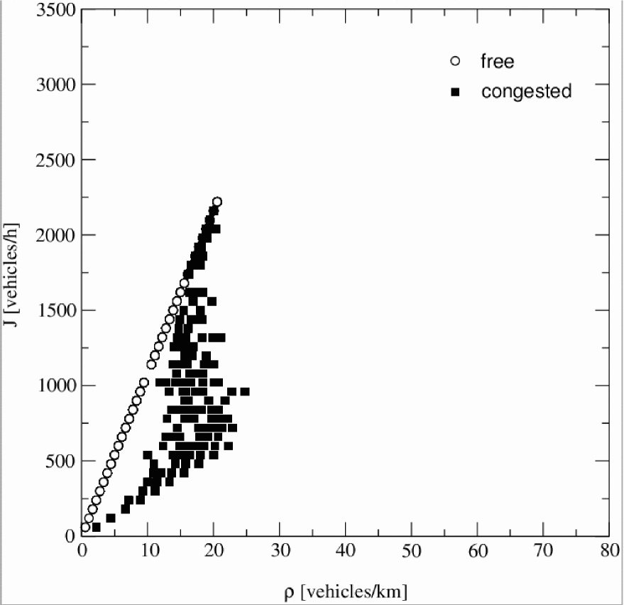
FIG. 11.: Fundamental diagram of the TOCA model. As discretization we used a cell length of $7.5$ m and a time-step corresponding to $\Delta t=1$ s in reality. The parameters of the model are chosen as $t_{s}=1.2$, $p_{\rm{ac}}=p_{\rm{dec}}=0.9$ and $v_{\rm{max}}=4~{}\rm{cells}/\Delta t=108$ km/h.

As expected for this parameterization of the model we obtain results for the fundamental diagram that are similar to the NaSch model (Fig. 11).

The absence of spontaneous velocity fluctuations at low densities, however, implies that $p_{\text{dec}}$ has to be chosen quite large in order to obtain realistic values of the maximal flow. At the same time large values of the braking probability lead to the formation of jams at low densities, such that it is difficult to obtain density fluctuations with amplitudes comparable to the empirically observed values.

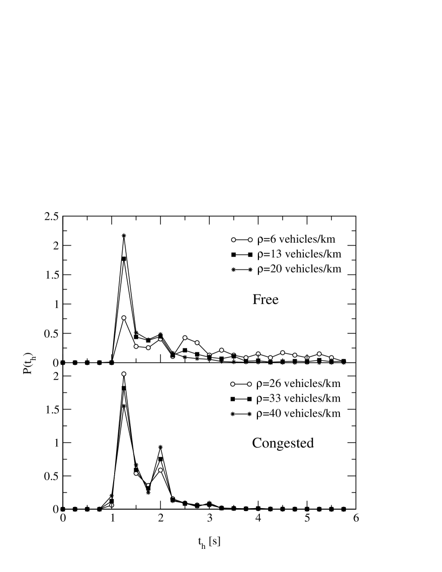
FIG. 12.: Normalized time-headway distribution for the TOCA model in free flow and congested traffic for different densities.

The time-headway distributions of the TOCA model, however, differ significantly from the results of the NaSch model (Fig. 12). For free flow traffic the position of the maximum is different from the minimal time-headway for the chosen set of parameters. The maximum coincides with $t_{h}$ while the minimal time-headway is determined by the unit of time. For congested traffic the distribution has two maxima, one corresponding to the typical time-headway in free flow traffic and the other corresponding to the typical temporal distance in the outflow region of a jam.

The OV functions of the TOCA and the NaSch model differ in two respects (Fig. 13). $(i)$ Due to the fact that the randomization step is applied for a finite range of the interactions, all cars move deterministically with $v_{\rm{max}}$ at low densities and therefore spatial headways smaller than $v_{\text{max}}$ cells are completely avoided. This result is at least partly a consequence of our simulation setup, i.e., choosing exactly the same maximal velocity for every car. $(ii)$ The second difference is found in the density dependence of the OV-function for congested traffic. Because of the retarded acceleration in step 1 and the deceleration of vehicles with $v\leq d$, at very large densities the system contains only one large jam with a width comparable to the system size. As a consequence, the mean velocity at a given distance is reduced considerably compared to free flow. The transition to a completely jammed system occurs at densities of about $66$ veh/km and leads to the abrupt change of the OV-curve.

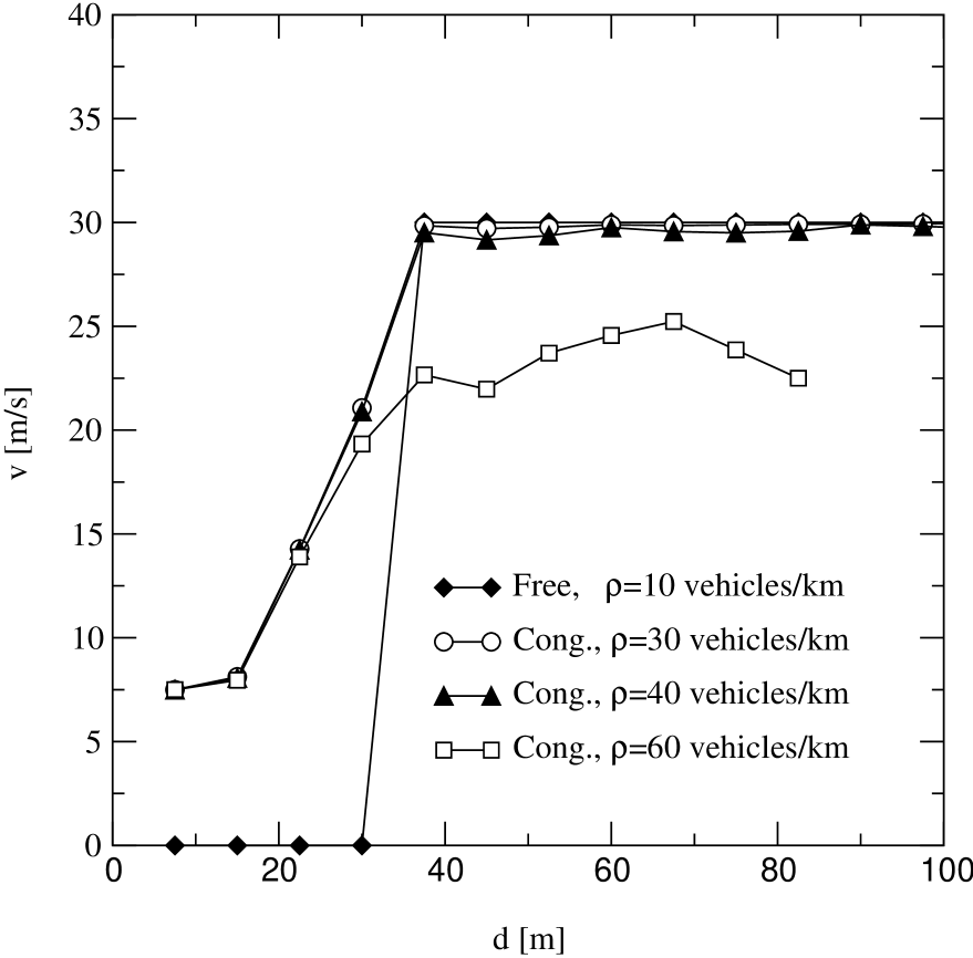
FIG. 13.: OV functions of the TOCA model in free flow and congested traffic for different densities.

The main difference between the NaSch model and the TOCA approach is the structure of jams. Due to the restricted application of the randomization step, $p_{\rm{dec}}$ must be quite large in order to obtain reasonable results for the fundamental diagram. Such a choice of $p_{\rm{dec}}$, however, reduces significantly the density of jams. This implies that, although the typical time-headway in the outflow region of a jam has the correct value, the downstream velocity of jams is too large.

Our analysis revealed several shortcomings of the TOCA model. However, we believe that the TOCA model is an interesting advancement of the NaSch model if a finer spatial discretization is applied. We will illustrate this for the example of the density of a wide jam: The inverse density of wide jams was used in order to fix the size of a cell. This choice is correct, as the jams in the model are basically compact, which is not true in case of the TOCA model. In this case more accurate results could be obtained if each cell would be divided into three cells. Using this finer discretization cars occupy two cells which would finally lead to a quite realistic dynamics of jams. A more elaborate discussion of the discretization effects can be found in appendix A.

IV CA models with modified distance rules

A The model of Emmerich & Rank

The CA model introduced by Emmerich and Rank [17] (ER-model) is another variant of the NaSch model with an enhanced interaction radius. Precisely speaking the braking rule of the NaSch model is replaced by applying a velocity dependent safety rule that is implemented via a gap-velocity matrix $M$. The entries $M_{ij}$ of $M$ denote the allowed velocities for a car with gap $i$ and velocity $j$. Replacing the braking rule $M_{ij}\leq j$ holds because otherwise the car would accelerate. For the NaSch model the elements of the gap-velocity matrix $M^{(\rm{NaSch})}$ simply read $M_{ij}=\min\{i,j\}$.

Emmerich and Rank tried to improve the NaSch model by introducing a larger interaction horizon, i.e. by an earlier adaption of the speed. This partly avoids the unrealistic effect, that drivers stop from a high speed within one time step. Compared to the Nasch model their choice of the matrix $M$ only modifies the distance rule for cars moving with velocity $v_{\text{max}}$: If $4\leq d\leq 9$ the car $n$ has to slow down to velocity $4$. For all other combinations of $d$ and $v$ the NaSch distance rule is left unchanged.

As a second modification of the NaSch model a different update scheme is applied. The ER model uses an unusual variant of the ordered sequential update, i.e., all rules, including the movement of the vehicles, are directly applied for the chosen car. A unit of time corresponds to one update of all cars. Ordered sequential updates use normally a fixed sequence of cars or lattice sites. This has the disadvantage that some observables, e.g., the typical headway, may depend on the position of the detection device, even for periodic systems. In order to reduce this effect the car with the largest gap is chosen first and than the update propagates against the driving direction [17].

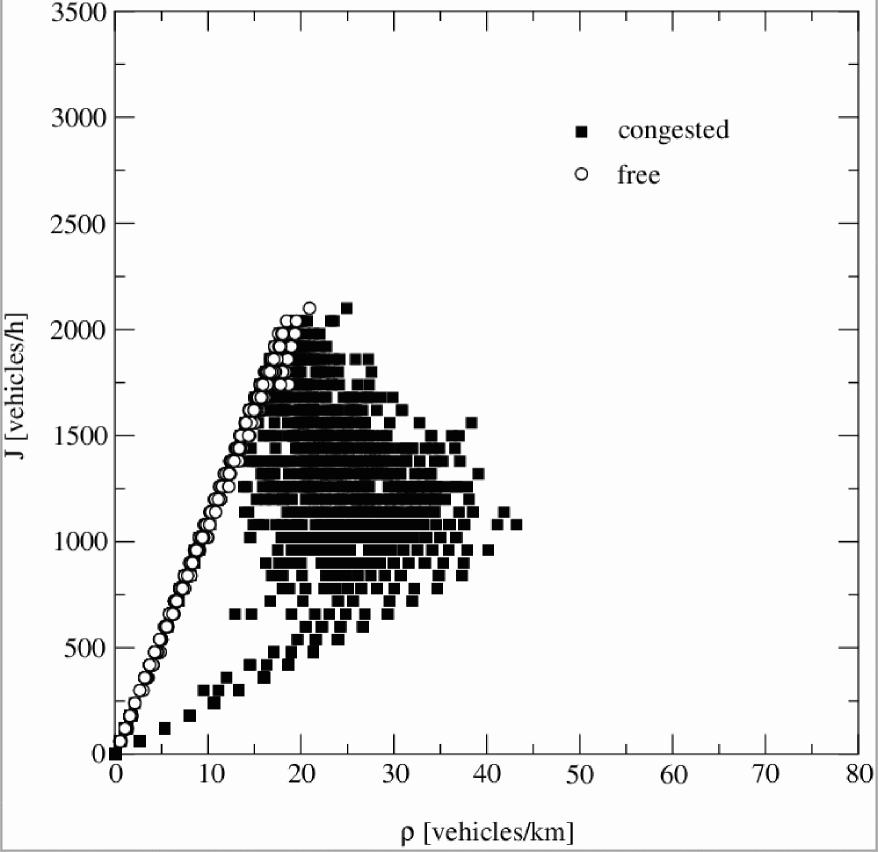
FIG. 14.: Fundamental diagram of the ER-model. As suggested in the original work we have chosen $7.5$ m as the length of a cell, $\Delta t=1$ s, $p_{\rm{dec}}=0.3$ and $v_{\rm{max}}=5=135$ km/h.

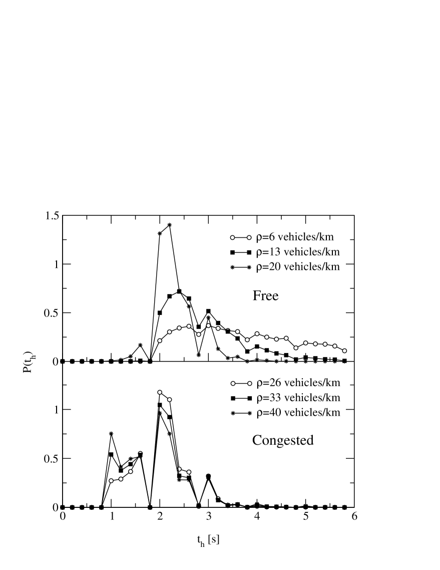
FIG. 15.: Normalized time-headway distribution for the ER model in free flow and congested traffic for different densities.

As a consequence of the ordered sequential update scheme, the gaps are used very efficiently and very large flows can be achieved [43]. (Now, it is allowed that two cars are driving with $v_{\rm{max}}$ and $d=0$, so that flows $J>1~{}\rm{veh}/{\Delta t}$ are possible). Therefore large deceleration probabilities are necessary to decrease the overall flow to realistic values. Nevertheless, due to the sequential update scheme, the spontaneous jam formation is reduced considerably. The application of a sequential update is crucial. If it is replaced, e.g., by a parallel update, one may observe an unrealistic form, i.e., a non-monotonous behavior, of the fundamental diagram at low densities [1].

Due to the special choice of $M^{(\rm{ER})}$, the velocity of cars with $d\leq 9$ is restricted to $v\leq 4$. This means, that a generic speed limit with $v_{\rm{max}}=4$ is applied for all densities $\rho\geq 1/11\approx 12$ veh/km, where the mean distance between the cars is smaller than $10$ cells. Therefore, the free flow branch of the fundamental diagram in Fig. 14 has in contrast to the empirical data two different slopes, one corresponding to $v_{\rm{max}}=5~{}\rm{cells}/\Delta t$ if $\rho<15$ veh/km and the other to $v_{\rm{max}}=5~{}\rm{cells}/\Delta t$ at larger densities.

For the present choice of $M$ we recover basically the distance rule of the NaSch model with $v_{\rm{max}}=4~{}\rm{cells}/\Delta t$, because the speed limit applies only for larger distances. Therefore the structure of the congested part of the fundamental diagram is quite similar to the NaSch model. However, important differences concerning the microscopic structure of the traffic state exist, mainly due to the modified update scheme. The ordered sequential update allows motion at high speeds and small distances. This could in principle (for small $p_{\rm{dec}}$) lead to very short time-headways. For the chosen value of $p_{\rm{dec}}$, however, the typical time-headways are quite large in the free flow regime and do not match the empirical findings. Nevertheless the ordered sequential update changes qualitatively the form of the time-headway distribution, i.e., the position of the maximum and the short time cut-off are different, as empirically observed (Fig. 15).

The OV-function of the ER-model differs strongly from the empirical findings (Fig. 16). For this quantity the modified distance rule is of great importance. In the congested regime, we observe plateaus of almost constant average velocities $v<v_{\rm{max}}$. The density dependence of the OV function is, as for the NaSch model, very weak. In free flow traffic small headways simply have not been observed, in contradiction to the empirical results.

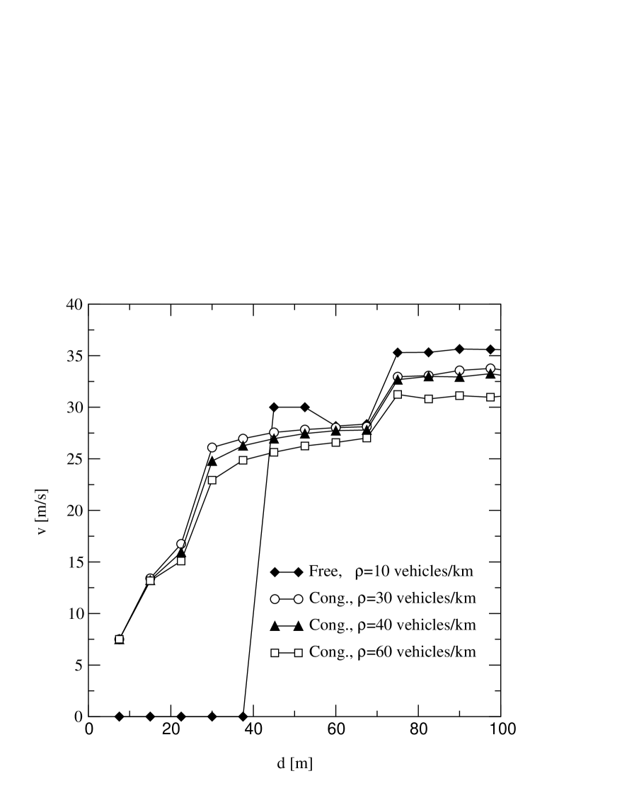
FIG. 16.: OV function of the ER model in free flow and congested traffic for different densities.

The most important weakness of the ER-model is its description of the jam dynamics. First of all for small values of $p_{\rm{dec}}$ the possibility of downstream moving jams exist, which contradicts all empirical studies. But even for the large value of $p_{\rm{dec}}$ we applied, jams are not stable, i.e., often branch into a number of small jams. Therefore it is impossible to reproduce the empirically observed parallel moving jams with the ER-model.

In summary, the gap-velocity matrix allows a more detailed modeling of the interaction horizon. But keeping the parallel update scheme, unrealistic behavior at low densities is observed. Using a special variant of the sequential update leads to a very unrealistic structure of the microscopic traffic states.

B A discrete optimal velocity model

Helbing and Schreckenberg (HS) [18] have introduced a cellular automata (CA) model for the description of highway traffic based on the discretization of the optimal-velocity (OV) model of Bando et al. [33]. The model was introduced in order to provide an alternative mechanism of jam formation. In certain density regimes the HS model is very sensitive to external perturbations due to its intrinsic nonlinearity. So in contrast to the previous approaches the pattern formation is of chaotic rather than of stochastic nature, although the definition of the model includes a stochastic part as well.

The deterministic part of the velocity update is done by assigning the following velocity to the cars:

$$v_{n}(t+1/2)=v_{n}(t)+\Big{\lfloor}\lambda[V_{\rm{opt}}(d_{n})-v_{n}(t)]\Big{\rfloor}$$ (4)

where $V_{\rm{opt}}(d)$ denotes the “optimal” velocity of car $n$ for a given distance $d_{n}$ to the vehicle ahead, $v_{n}(t)$ the discrete velocity at time $t$ and $\lfloor\dots\rfloor$ the floor function. The constant $\lambda$ is a free parameter of the model. The acceleration step is the naive discretization of the acceleration step of the space and time continuous OV model. In the continuous version of the OV model the parameter $\lambda$ determines the timescale of the acceleration. However, for time-discrete models it is well known that a simple rescaling of time is not possible. Therefore the meaning of the parameter $\lambda$ remains unclear.

The deterministic update is followed by a randomization step as known from the NaSch model, i.e. the velocity of a car with $v_{n}(t+1/2)>0$ is reduced with probability by one unit.

Although the definition of the model seems to be quite similar to the models discussed in the previous sections, important differences exist. In all other models discussed so far acceleration is limited to one velocity unit per time-step while breaking from $v_{\text{max}}$ to zero velocity is possible. This is not true for the HS model where a standing car may accelerate towards $\lfloor\lambda V_{\rm{opt}}(\infty)\rfloor>1$ in a single time-step. On the other hand, in particular for small values of $\lambda$, the braking capacity of cars is reduced. A reduced braking capacity, however, may lead to accidents (see the discussion in [13, 44, 45]), a certainly unwanted feature of a traffic model. It also implies that the model is not defined completely by the dynamics. This becomes a problem especially in simulations. Here further rules are necessary to determine how to deal with accidents.

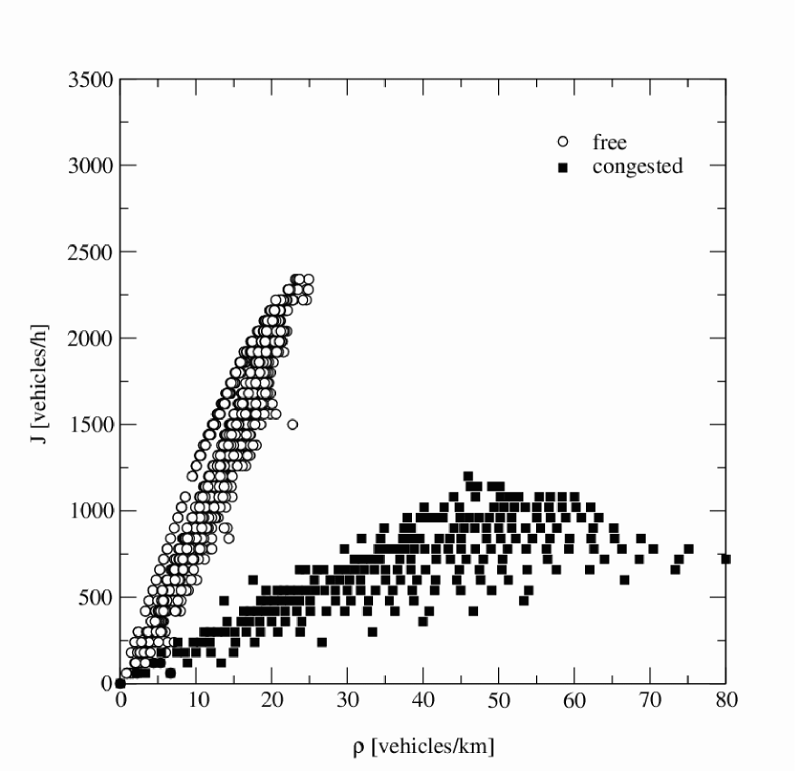
FIG. 17.: Fundamental diagram of the HS-model. As suggested in the original work we have chosen $2.5$ m as the length of a cell, a vehicle has a length of $2$ cells, $\Delta t=1$ s, $p_{\rm{dec}}=0.001$, $v_{\rm{max}}=15=135$ km/h and $\lambda=1/1.3$.

We will discuss the possibility of accidents in some more detail in appendix B. This discussion concentrates on a criterion which ensures that for any possible initial condition no accident occurs.

In [18] for comparison with empirical data the following OV-function is suggested:

$d$ $[\Delta x]$	$OV(d)$ $[\Delta x/\Delta t]$	$d$ $[\Delta x]$	$OV(d)$$[\Delta x/\Delta t]$
0, 1	0	11	8
2,3	1	12	9
4,5	2	13	10
6	3	14,15	11
7	4	16–18	12
8	5	19 – 23	13
9	6	24 – 36	14
10	7	$\geq 37$	15

The length of a cell is set to $\Delta x=2.5$ m, $\Delta t=1$ is chosen as the unit of time, $\lambda=\frac{1}{1.3}$ and we used the randomization probability $p_{\rm{dec}}=0.001$ as suggested in [18]. A vehicle has a length of $l=2~{}$cells corresponding to $5$ m. For this choice of $\lambda$ and the OV function the model is not strictly free of collisions as our discussion in the appendix shows, but does at the same time not lead to accidents if an appropriate initial condition is chosen and the density is not too high.

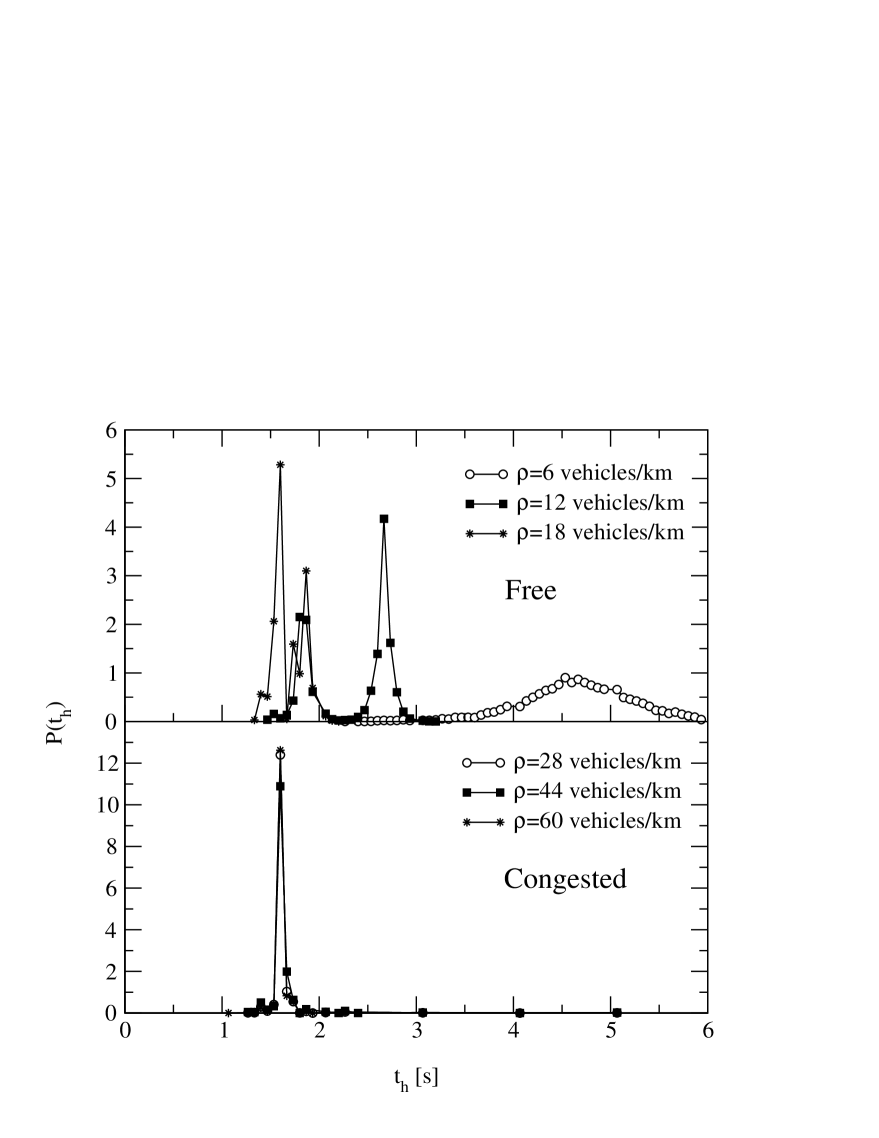
FIG. 18.: Normalized time-headway distribution for the HS model in free flow and congested traffic for different densities.

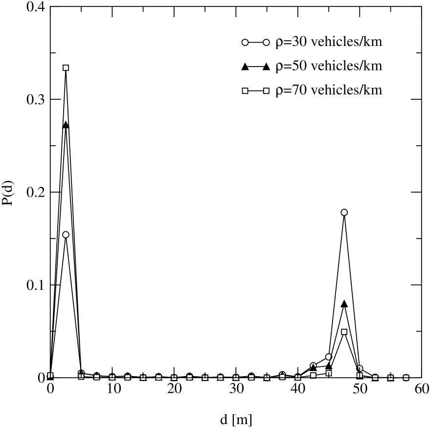
FIG. 19.: Distance headway distributions in the congested regime. Obviously non-compact jams coexist with free flow regimes, where the distance between two cars is rather large.

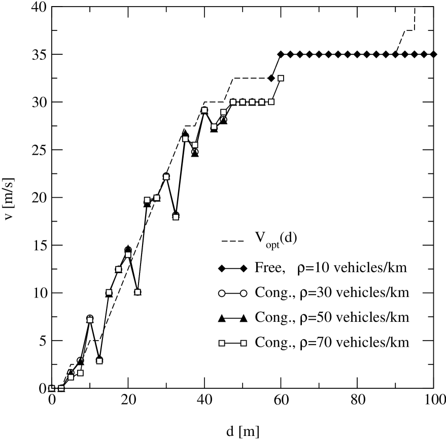
FIG. 20.: OV function of the HS model in free flow and congested traffic for different densities.

The optimal velocity function that governs the deterministic part of the vehicle dynamics, leads to speed limits in certain density regimes $l/(d_{\rm{max}}+l)<\rho<l/(d_{\rm{min}}+l)$ with $V_{\rm{opt}}(d_{\rm{min}})=V_{\rm{opt}}(d_{\rm{max}})$. These different optimal speeds become visible in different slopes in the free flow branch of the fundamental diagram (Fig. 17). For congested traffic two different traffic regimes can be identified, as empirically observed. For very high densities, one observes a reasonable agreement with the empirical data, i.e. the form of the jammed branch is reproduced qualitatively. This branch of the fundamental diagram is, however, observed only in a very narrow interval of global densities.

Compared to the two other traffic states the reproduction of synchronized traffic is rather poor. First, one obviously observes a strong correlation between density and flow, which is contrast to the empirical findings, and second, the range of densities which is observed in local measurements is quite narrow.

The main difficulties of the model are visible when comparing it with empirical results on a microscopic level. The simulations for the time-headway distribution show a strong density dependence of the maximum for the free flow states. This is due to the long-ranged interactions that tend to generate traffic states that are very homogeneous. Therefore short time-headways are suppressed at low densities. The second problem is the quasi-deterministic character of the model. This implies that drivers obey the distance rule in almost any case. As a result the peak values of the time-headway distribution have extremely high weights. In congested traffic we observe a density independent position of the maximum of the time-headway distribution. The maximum carries almost the whole weight of the distribution, in contradiction to the empirical findings. The reason for this can be read off from the distance headway distributions for different global densities (Fig. 19). Within a large density regime we observe coexistence of non-compact jams and free flow traffic. Therefore we can state that both high density states correspond to stop-and-go traffic, i.e. the model fails to reproduce synchronised traffic at all.

The mismatch of the model and empirical structure of traffic states is also obvious for the OV-function (Fig. 20). It shows almost no density dependence and is basically independent of the traffic state. The difference between the different curves is only in a density dependent cut-off of the distribution, i.e. at high densities large distances simply do not occur.

The simulations show that HS model fails to reproduce the microscopic structure of the empirical observed traffic states. From our point of view the problems describing the empirical observation are due to the nature of the model. It introduces a static rule that leads to a reasonable agreement with the empirical fundamental diagram. For a proper choice of $\lambda$ the vehicles take instantaneously a velocity close to the optimal velocity, i.e. the dynamical aspects of highway traffic are extremely simplified. Therefore inhomogeneous traffic states are only observed in the presence of quenched disorder [18], e.g. different types of cars, and not produced spontaneously.

V Brake light version of the NaSch model

Quite recently a brake light (BL) version of the NaSch model has been introduced  [19, 20] in order to give a more complete description of the empirically observed phenomena in highway traffic. In contrast to the models we considered in the previous sections, which represent already well known modeling approaches, we also discuss the basic features of the model that have not been presented so far. In the development of the model the main aim was the reproduction of the empirical microscopic data in a robust way.

A Definition of the BL model

The BL model combines several elements of older modeling approaches, e.g., velocity anticipation [46, 47] and a slow-to-start rule [39, 15]. In addition, a dynamical long ranged interaction is included: In their velocity dependent interaction horizon drivers react on brakings of the leading vehicle that are indicated by an activated brake light [48]. The interaction, however, is limited to nearest neighbor vehicles [49]. The update rules are formulated in analogy to the VDR model. In particular the interactions are strictly local and a parallel update scheme is applied.

In order to allow for a finer spatial discretization for a given length of a car, we include the possibility that a car may occupy more than a single cell. Therefore the gap between consecutive cars is given by $d_{n}=x_{n+1}-x_{n}-l$ (where $l$ is the length of the cars). The brake light $b_{n}$ can take on two states, i.e., on (off) indicated by $b_{n}=1(0)$. In our approach the randomization parameter $p_{\rm{dec}}$ for the $n$th car can take on three different values $p_{0}$, $p_{d}$ and $p_{b}$, depending on its current velocity $v_{n}(t)$ and the status $b_{n+1}$ of the brake light of the preceding vehicle $n+1$:

$$p_{\rm{dec}} = p_{\rm{dec}}(v_{n}(t),b_{n+1}(t),t_{h},t_{s})$$ (5)

$$= \left\{\begin{array}[]{llll}p_{b}&&{\rm if\ }b_{n+1}=1{\rm\ and\ }t_{h}<t_{s}\\ p_{0}&&{\rm if\ }v_{n}=0\\ p_{d}&&{\rm in\ all\ other\ cases}.\end{array}\right.$$ (9)

The two times $t_{h}=\frac{d_{n}}{v_{n}(t)}$ and $t_{s}=\min\{v_{n}(t),h\}$, where $h$ determines the range of interaction with the brake light, are the time $t_{h}$ needed to reach the position of the leading vehicle which has to be compared with a velocity-dependent (temporal) interaction horizon $t_{s}$. $t_{s}$ introduces a cutoff that prevents drivers from reacting to the brake light of a predecessor which is very far away. Finally $d_{n}^{(\rm{eff})}=d_{n}+\max\{v_{\rm{anti}}-d_{\rm{security}},0\}$ denotes the effective gap where $v_{\rm{anti}}=\min\{d_{n+1},v_{n+1}\}$ is the expected velocity of the leading vehicle in the next time-step. The effectiveness of the anticipation is controlled by the parameter $d_{\rm{security}}$. Accidents are avoided only if the constraint $d_{\rm{security}}\geq 1$ is fulfilled. The update rules then are as follows ($t<t_{1}<t_{2}<t+1$):

1. Determination of the randomization parameter:
   $p_{\rm{dec}}=p_{\rm{dec}}(v_{n}(t),b_{n+1}(t),t_{h},t_{s})$
   $b_{n}(t+1)=0$
   

2. Acceleration:
   if $\bigl{(}(b_{n+1}(t)=0)$ and $(b_{n}(t)=0)\bigr{)}$ or $(t_{h}\geq t_{s})$ then
       $v_{n}(t_{1})=\min\{v_{n}(t)+1,v_{\rm{max}}\}$
   

3. Braking rule:
   $v_{n}(t_{2})=\min\{d_{n}^{(\rm{eff})},v_{n}(t_{1})\}$
   if $(v_{n}(t_{2})<v_{n}(t))$ then
       $b_{n}(t+1)=1$
   

4. Randomization, brake:
   if $({\rm rand}()<p_{\text{dec}})$ then $\{$
       $v_{n}(t+1)=\max\{v_{n}(t_{2})-1,0\}$
       if $((p_{\text{dec}}=p_{b})\textrm{ and }(v_{n}(t+1)=v_{n}(t_{2})-1))$ then
         $b_{n}(t+1)=1\}$
   

5. Car motion:
   $x_{n}(t+1)=x_{n}(t)+v_{n}(t+1)$
   

Here rand$()$ denotes a uniformly distributed random number from the interval $[0,1]$.

The new velocity of the vehicles is determined by steps $1-3$, while step $0$ determines the dynamical parameters of the model. Finally, the position of the car is shifted in accordance with the calculated velocity in step 4.

In order to illustrate the details of the approach we now discuss the update rules step-wise.

1. The braking parameter $p_{\rm{dec}}$ is calculated. For a stopped car the value $p_{\rm{dec}}=p_{0}$ is applied. Therefore $p_{0}$ determines the upstream velocity of the downstream front of a jam.

   If the brake light of the car in front is switched on and it is found within the interaction horizon $p_{\rm{dec}}=p_{b}$ is chosen. A car perceives a brake light of the vehicle ahead within a time dependent interaction horizon $t_{s}=\min\{v_{n}(t),h\}$ where $v_{n}(t)$ is the current velocity and $h$ an integer constant. The velocity dependence takes into account the increased attention of the driver at large and reduces the braking readiness at small velocities. This reaction is performed only with a certain probability of $p_{b}$. In order to obtain a finite range of interactions a cutoff at a horizon of $h$ seconds is made .

   Finally, $p_{\rm{dec}}=p_{d}$ is chosen in all other cases.

2. The velocity of the car is increased by one unit (if it does not already move with maximum velocity). The car does not accelerate if its own brake light or that of its predecessor is on and the next car ahead is within the interaction horizon.

3. The velocity of the car is adjusted according to the effective gap.

   The brake light of a vehicle is activated only if the new velocity is reduced compared to the preceding time-step. Note that the application of the braking rule does not necessarily lead to a change of the velocity, as it can compensate a previous acceleration. The restriction stabilizes dense traffic flows.

4. The velocity of the car is reduced by one unit with a certain probability $p_{\rm{dec}}=p_{\rm{dec}}(v_{n}(t),b_{n+1},t_{h},t_{s})$. If the car brakes due to the predecessor’s brake light, its own brake light is switched on. We also stress the fact that even for distances $d_{n}<h$ the action of the brake light is restricted to brakings that are induced by the vehicle in front (either by the braking rule or by an activated brake light) and not by spontaneous velocity fluctuations.

5. The position of the car is updated.

B Calibration of the model

The following parameters of the model allow to adjust the simulation data to the empirical findings: the maximal velocity $v_{\rm{max}}$, the car length $l$, the braking parameters $p_{d}$, $p_{b}$, $p_{0}$, the cut-off $h$ of interactions, and the minimal security gap $d_{\rm{security}}$. The parameters of the have been chosen such that they can easily be related to the empirical findings. As in the previous models a single set of parameters is used for all traffic states.

In order to obtain realistic values of the acceleration behavior of a vehicle, the cell length of the standard CA model is reduced to a length $l$ of $1.5$ m. Since the time-step is kept fixed at a value of $1$ s this leads to a velocity discretization of $1.5$ m/s which is of the same order as the ”comfortable” acceleration of somewhere about $1~{}\rm{m/s}^{2}$ [50]. Like in the standard CA model a vehicle has a length of $7.5$ m that corresponds to $5$ cells at the given discretization (see appendix A for a discussion of the discretization effects).

Some of the parameters can be fixed as, e.g., in the VDR-model: The maximum velocity $v_{\rm{max}}$ is determined by the slope of the free flow branch of the fundamental diagram. The upstream velocity of a jam can be tuned by the parameter $p_{0}$ and the strength of fluctuations that are controlled by the parameter $p_{d}$ determine the maximal flow.

The other parameters of the model are connected with an interaction that have not been included in the models we discussed so far. The parameter $h$ describes the horizon above which driving is not influenced by the leading vehicle. Several empirical studies reveal that $h$ corresponds to a temporal headway rather than to a spatial one. The estimates for $h$ vary from $6$ s [51], $8$ s [52, 53], $9$ s [54] to $11$ s [55]. Another estimation for $h$ can be obtained from the analysis of the perception sight distance. The perception sight distance is based on the first perception of an object in the visual field at which the driver perceives movement (angular velocity). In [56] velocity-dependent perception sight distances are presented that, for velocities up to $128$ km/h, are larger than $9$ s. We therefore have chosen $h$ to be $6$ s as a lower bound for the time-headway. Besides, our simulations show, that a good agreement with empirical data can only be obtained for $h\geq 6$. This corresponds to a maximum horizon of $6\times 20$ cells or a distance of $180$ m at velocity $v_{\rm{max}}$.

The next parameter one has to fix is $p_{b}$. This parameter controls the propagation of the brake light. A braking car in front is indeed a strong stimulus to adjust the own speed. Therefore $p_{b}$ has typically a high value. Finally, $d_{\rm{security}}$ tunes the degree of the velocity anticipation and has a strong influence on the cut-off of the time-headway distribution.

C Validation of the full model

With this parameter set we have calibrated the model to the empirical data. Leaving $p_{0}$, $h$ and $v_{\rm{max}}$ fixed, we got the best agreement with the empirical data for $p_{\rm{dec}}=0.1$, $p_{b}=0.94$ and $d_{\rm{security}}=7$.

As one can see in Fig. 21 the slope of the free flow branch and the maximum flow coincides with the empirical data indicating that $v_{\rm{max}}$ and $p_{\rm{dec}}$ have been chosen properly.

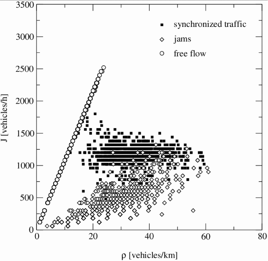
FIG. 21.: Local fundamental diagram obtained by the simulation of the brake light version of the NaSch model. The parameters are: $p_{0}=0.5$, $h=6$, $v_{\rm{max}}=20$, $p_{\rm{dec}}=0.1$, $p_{b}=0.94$, $d_{\rm{security}}=7$. A time-step corresponds to $\Delta t=1$ s, a cell has a length $l=1.5$ m and a vehicle covers $5$ cells.

However, the simulated densities are less distributed than in the empirical data set. The width of the density distribution is of the same order as it was found for the NaSch and ER-model. The mismatch between simulation and empirical results of the density can be related to discretization effects, which introduce an upper limit for the density if simple (virtual) counting loops are used as detection devices.

A second lower branch appears for small values of the flow which represents wide jams. Because only moving cars are measured by the inductive loop large densities cannot be calculated, as in the empirical data of Fig. 1.

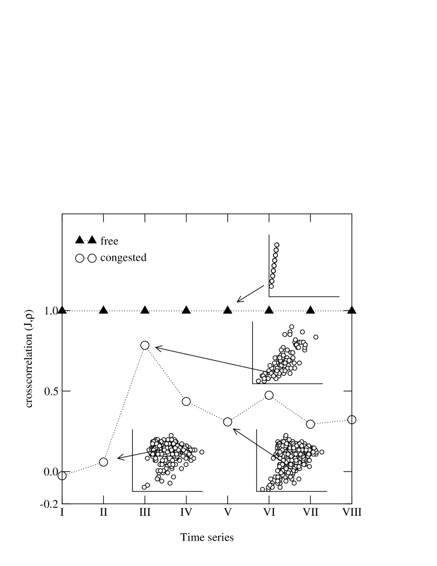
FIG. 22.: Cross-correlation of the flow and the density in free flow and congested traffic for different densities and homogeneous initialization.

The next parameter that can be directly related to an empirical observable quantity, namely the upstream velocity of the downstream front of a wide jam, is the deceleration probability $p_{0}$.

We used the calculation of the density autocorrelation function in the congested state of a system that was initialized with a mega jam for the determination of the velocity of the jam front. One obtains an average jam velocity of $2.36$ cells/s $(\hat{=}12.75~{}\rm{km/h})$ for $p_{0}=0.5$. This jam velocity is independent of the traffic condition and holds for all densities in the congested regime. Thus, although metastable traffic states can be achieved by the finer discretization (see appendix A) the slow-to-start rule is necessary for the reduction of the jam velocity from about $20.45$ km/h to $12.75$ km/h. This velocity is also in accordance with empirical results [32].

In Fig. 22 the cross-covariance $cc(J,\rho)$ of the flow and the local measured density for different traffic states is shown. In the free flow regime the flow is strongly coupled to the density indicating that the average velocity is nearly constant. Also for large densities, when wide jams are measured, the flow is mainly controlled by density fluctuations. In the mean density region there is a transition between these two regimes. At cross-covariances in the vicinity of zero the fundamental diagram shows a plateau. Traffic states with $cc(J,\rho)\approx 0$ were identified as synchronized flow [22]. In the further comparison of our simulation with the corresponding empirical data we used these traffic states for synchronized flow data and congested states with $cc(J,\rho)>0.7$ for data of wide jams. The results show that the approach leads to realistic results for the fundamental diagram and that the model is able to reproduce the three different traffic states.

To characterize the three traffic states, we calculated the autocorrelation of the flow, the density as well as the velocity for different global densities.

In free flow, the density and the flow show the same oscillations of the autocorrelation function, whereas the speed is not correlated in time.

In contrast to the NaSch model, the autocorrelation function at large densities shows a strong coupling of the flow and the velocity. Now, the velocity of a car not only depends on the gap but also on the density, so that the flow and the velocity are mainly controlled by the density (Fig. 23).

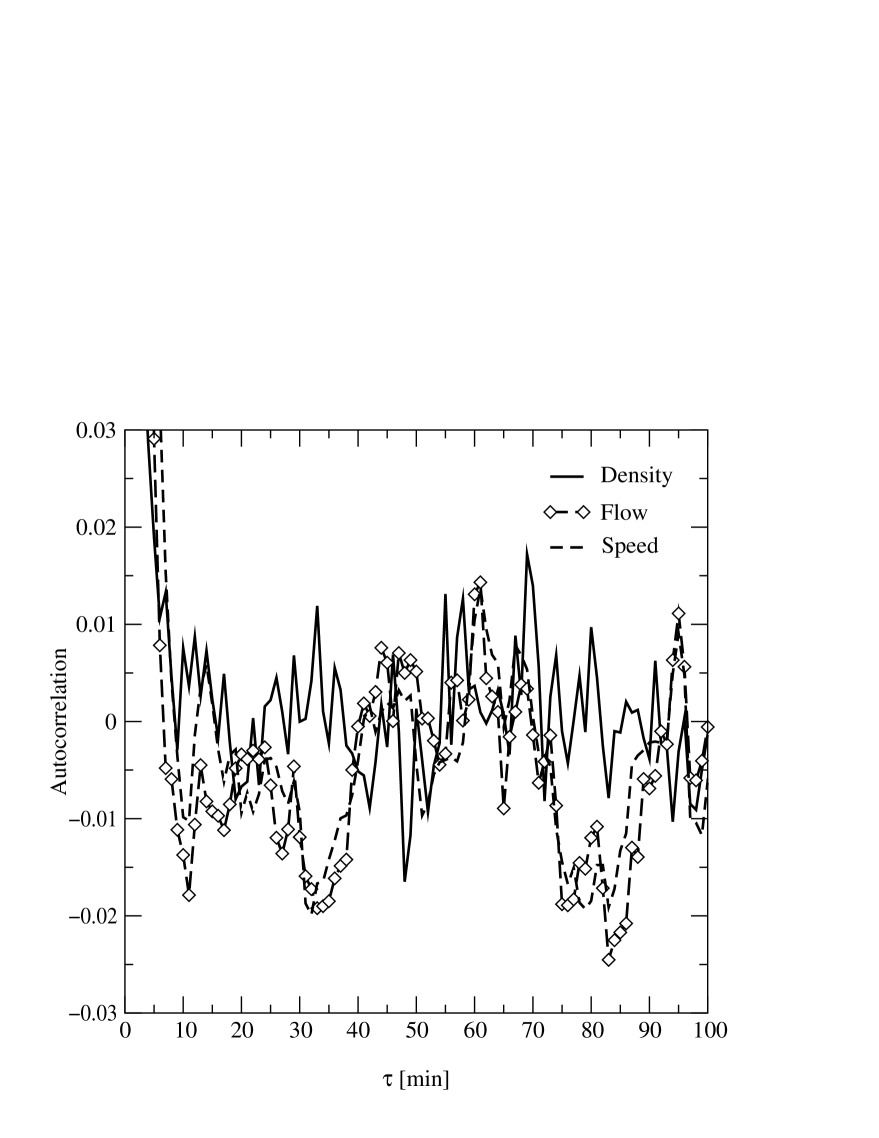
FIG. 23.: Autocorrelation function of the density, the velocity and the flow for $\rho=67$ veh/km with a random initialization.

Next we compare the empirical data and simulation results on a microscopic level.

In Fig. 24 the simulated time-headway distributions for different density regimes are shown.

Due to the discrete nature of the model, large fluctuations occur and the continuous part of the empirical distribution shows a peaked structure at integer-numbered headways for the simulations. In the free flow state extremely small time-headways have been found, in accordance with the empirical results. This is qualitatively different from the other CA models with parallel update scheme.

FIG. 24.: Time-headway distribution for different densities in free flow (top) and in the synchronized state (bottom).

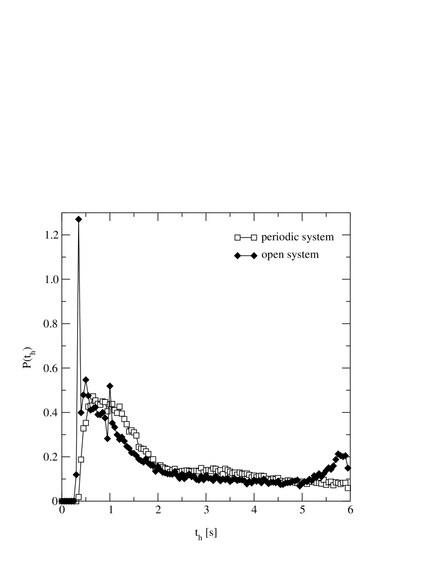
FIG. 25.: Time-headway distribution in the free flow regime of a system with open boundary conditions and different types of vehicles. The maximal velocity of the slow vehicles was set to as $v_{\rm{max}}=108~{}\rm{km/h}=20$ cells/s and of the fast vehicles as $v_{\rm{max}}=135~{}\rm{km/h}=25$ cells/s. We considered $15\%$ of the vehicles as fast vehicles (note that these are vehicles that disregard the speed limit).

Nevertheless, for our standard simulation setup at small densities the statistical weight of these small time-headways is significantly underestimated. This apparent failure of the model is the result of the chosen simulation setup. If we introduce different types of cars and open boundary conditions, we observe a smooth time headway distribution, which is in good agreement with the empirical data (see Fig. 25). Therefore we can state that properties like the width as well as the smoothness of the time-headway distribution are strongly dependent on the choice of the simulation setup. In contrast, the short-time cut-off of the distribution is model dependent. Time headways shorter than the chosen unit of time are in case of a parallel update only observed if anticipation effects are included. The actual value of the cut-off for a given unit of time is tuned by the parameter $d_{\rm{security}}$. The results for congested flow, however, are not influenced by different types of vehicles.

The ability to anticipate the predecessor’s behavior becomes weaker with increasing density so that the weight of the small time-headways is reduced considerably in the synchronized state. The maximum of the distribution can be found in the vicinity of $1$ s in accordance with the empirical data, the density dependence, however, cannot be reproduced.

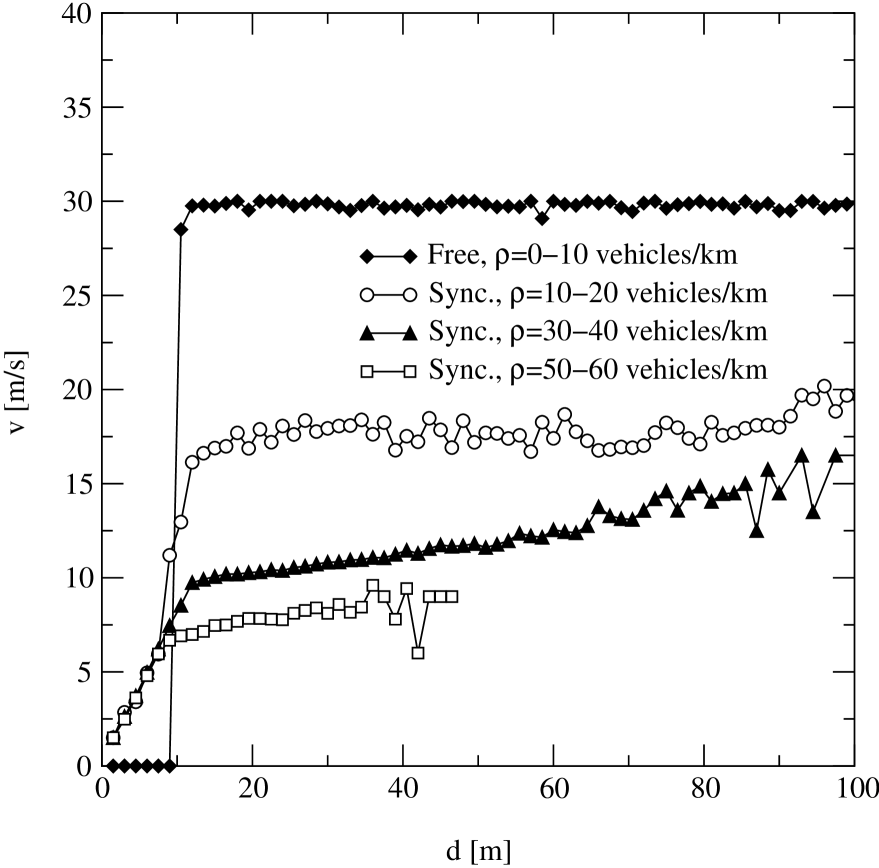
FIG. 26.: The OV-function for different densities in the free flow and congested regime.

Instead, with increasing density the maximum at a time of $1$ s (in the NaSch model the minimal time-headway is restricted to $1$ s because of rule 2) becomes more pronounced. This result is also due to the discretization of the model that triggers the spatial and temporal distance between the cars. Because of the exponential decay of the waiting time distribution of cars leaving a jam, the peak at a time of $1$ s is the most probable in the time-headway distribution.

The OV curve of our model approach shows an excellent agreement with empirical findings. For densities in the free flow regime it is obvious that the OV-curve (Fig. 26) deviates from the linear velocity-headway curve of the NaSch model. Due to anticipation effects, smaller distances occur, so that driving with $v_{\rm{max}}$ is possible even within very small headways. This strong anticipation becomes weaker with increasing density and cars tend to have smaller velocities than the headway allows so that the OV-curve saturates for large distances.

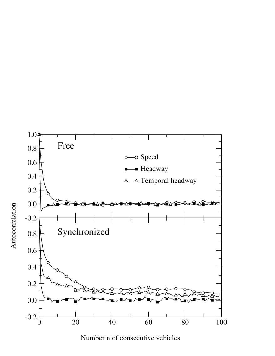
FIG. 27.: Autocorrelation of the speed and of the spatial and temporal headway for free flowing vehicles (top) and for a synchronized state (bottom). In order to obtain a slow decay of the speed autocorrelation function in the free flow regime the simulation was performed on a open system with $20\%$ of slow cars ($v_{\rm{max}}^{\rm{slow}}=15~{}\rm{cells/s}=81$ km/h, $v_{\rm{max}}^{\rm{fast}}=20~{}\rm{cells/s}=108$ km/h.)

The saturation of the velocity, which is characteristic for synchronized traffic, was not observed in earlier approaches. The value of the asymptotic velocities can be adjusted by the last free parameter $p_{b}$. The OV-curve in the synchronized regime is independent of the maximum velocity and is only determined by the dynamical behavior of the model.

Next, we calculated the autocorrelation of the time-series of the single-vehicle data (Fig. 27). Note, that the data of the free flow state was collected in an open system with $20\%$ of slow cars with $v_{\text{max}}=15$ cells/s = $81$ km/h. In the free flow regime the data shows a strong coupling of the spatial and temporal headway that supports the results obtained by aggregated data ($J\propto\Delta t^{-1}$ and $\rho\propto\Delta x^{-1}$). In contrast, the autocorrelation of the velocity shows a slow asymptotic decay. This supports the explanation of [22] that the slow decrease for small distances is due to small platoons of fast cars led by one slow car. In the synchronized state, longer correlations of the speed and the spatial headways can be observed. So, similar to the free flow regime, in the synchronized regime platoons of cars appear that are moving with the same speed [24].

VI The model of Kerner, Klenov and Wolf

The most recent modeling approach we include in our comparison was introduced by Kerner, Klenov and Wolf (KKW) [21]. This model is a fully discretized version of the space-continuous microscopic model introduced by Kerner and Klenov [58]. It combines, as the BL model, elements of car-following theory with the standard distance-dependent interactions. It is defined by an update rule including a deterministic and a stochastic part. The deterministic rule, which reads ($t<t_{1}<t+1$)

$$v_{n}(t_{1})=\max\biggl{\{}0,\min\{v_{\rm max},v_{\text{safe}}(t),v_{\text{des}}(t)\}\biggr{\}},$$ (10)

is applied first. The three velocities appearing are the free flow or maximal speed of the cars $v_{\rm max}$, the safe velocity $v_{\text{safe}}(t)$ and finally the desired velocity $v_{\text{des}}(t)$. $v_{\text{safe}}(t)$ is the velocity which guarantees collision-free motion and is simply the gap to the preceeding car, $v_{\text{safe}}(t)=d_{n}(t)$. It is the introduction of $v_{\text{des}}(t)$ which makes the difference to the NaSch model. The velocity $v_{\text{des}}(t)$ is given by

$$v_{\text{des}}(t)=\left\{\begin{array}[]{ll}v_{n}(t)+a&\quad\textrm{for }d_{n}>D(v_{n}(t))-l,\\ v_{n}(t)+\Delta(t)&\quad\textrm{for }d_{n}\leq D(v_{n}(t))-l.\\ \end{array}\right.$$ (11)

The calculation of $v_{\text{des}}(t)$ replaces the acceleration step of the NaSch model by a more complex rule. Here $l$ is the length of the vehicles and $D(v)$ a synchronization distance. The authors suggested a linear

$$D(v)=D_{0}+kv.$$ (12)

and a quadratic form

$$D(v)=D_{0}+v+\beta v^{2}$$ (13)

for the velocity dependent interaction range. Apart from the task of choosing an appropriate function, two model parameters are introduced in both cases. So far no systematic analysis of traffic data exist which leads empirically based parameter values or the functional forms. This could be done, at least in principle, by an extensive analysis of floating-car measurements. Moreover, the results in [21] show that the results agree at least qualitatively for both functions (12), (13) which have been considered.

The interaction range has been introduced as a synchronization radius, i.e. $D(v)$ is the distance which separates free driving cars from cars which already adjust their velocity according to the vehicle ahead. For large distances to the vehicle ahead, $d_{n}>D(v_{n}(t))-l$, the calculation of $v_{\text{des}}$ is equivalent to the acceleration step of the NaSch model. Inside the enlarged interaction radius, however, $v_{\text{des}}$ depends on the velocity of the leading car. Explicitely $\Delta(t)$ is given by

$$\Delta(t)=\left\{\begin{array}[]{ll}-b&\quad\textrm{if $v_{n}(t)>v_{n+1}(t)$}\\ 0&\quad\textrm{if $v_{n}(t)=v_{n+1}(t)$}\\ a&\quad\textrm{if $v_{n}(t)<v_{n+1}(t)$},\end{array}\right.$$ (14)

This means that within the interaction radius drivers tend to adapt their velocity to the vehicle ahead.

The second update rule is stochastic. It is given by

$$v_{n}(t+1)=\max\bigl{\{}0,\min\{v_{n}(t_{1})+\eta_{n},v_{n}(t_{1})+a,v_{\rm free},v_{\text{max}}\}\bigr{\}},$$ (15)

The stochasticity is included in the term $v_{n}(t_{1})+\eta_{n}$, while the others are in order to guarantee that the new velocity is below the speed limit, leads to no collisions and is in accordance with the chosen acceleration capacity $a_{n}$ of the cars. The stochastic variable $\eta$ can take the following values:

$$\eta=\left\{\begin{array}[]{ll}-1&\textrm{\ \ if $r<p_{\rm b}$},\\ 1&\textrm{\ \ if $p_{\rm b}\leq r<p_{\rm b}+p_{\rm a}$},\\ 0&\textrm{\ \ otherwise}\end{array}\right.$$ (16)

Both probabilities $p_{\rm a}$ and $p_{\rm b}$ introduced here are velocity dependent. One has

$$p_{{\rm b}}(v)=\left\{\begin{array}[]{ll}p_{0}&\textrm{\ \ if $v=0$}\\ p&\textrm{\ \ if $v>0$}.\end{array}\right.$$ (17)

with $p_{0}>p$. The stochastic braking is analogous to the slow-to-start rule known from the VDR model. Contrary the stochastic acceleration is a new feature of the model which weakens the synchronization of speeds as it applies to cars which reduced or kept their velocity although safe driving would have allowed a larger velocity. The function $p_{a}(v_{n})$ is explicitly given by

$$p_{\rm a}(v)=\left\{\begin{array}[]{ll}p_{\rm a1}&\textrm{\ \ if $v<v_{\rm p}$}\\ p_{\rm a2}&\textrm{\ \ if $v\geq v_{\rm p}$},\end{array}\right.$$ (18)

where $v_{\rm p}$, $p_{\rm a1}$ and $p_{\rm a2}<p_{\rm a1}$ are adjustable parameters of the model. The different probabilities have to be chosen such that $p_{a}+p_{b}\leq 1$ is fulfilled for any velocity. The velocity update is completed by this second stochastic rule and is followed by a parallel update of the positions.

For further illustration of the update rules we compare them briefly to the BL model. Both models include the update rules of the VDR model and enlarge the interaction radius of the drivers within a velocity dependent interaction range. The driving strategy within this larger interaction range is, however, different. While the BL model introduces an event driven interaction model, the KKW is more car-following like. Another important difference is that the velocity anticipation is not included in the approach of [21], although such an extension is possible [59].

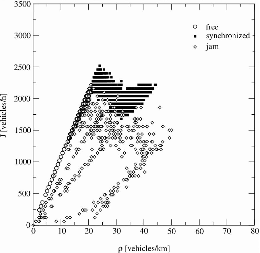
FIG. 28.: Local fundamental diagram of the KKW model for the following set of parameters: The length of a cell is set to $0.5~{}\rm{m}$. Each car occupies $l=15$ cells. The maximal velocity is given by $v_{\text{max}}=108~{}\rm{km/h}=60~{}\rm{cells}/\Delta t$, where $\Delta t=1~{}\rm{s}$. Also the other model parameters are set to the values suggested in [21]: $a=b=1$, $D_{0}=60$, $k=2.55$. The parameters determining the stochastic part of the model take the values: $p=0.04$, $p_{0}=0.425$, $p_{\text{a}1}=0.2$, $p_{\text{a}2}=0.052$ and $v_{p}=28$.

Fig. 28 shows the fundamental diagram of the KKW model, obtained by local measurements flux and density in a periodic system. Compared to the other models we analyzed one observes two remarkable differences: In synchronized traffic the flow has a local minimum for a density of $30~{}$veh/km and reaches a second maximum for a density of $40~{}$veh/km. The origin of this structure lies in the stochastic acceleration of cars which reduces considerably the probability to form a jam. A second important feature is the complex structure of the fundamental in the presence of jams. For very high global densities one observes all three traffic states at the same time and no strict phase separation as, e.g., in case of the VDR model.

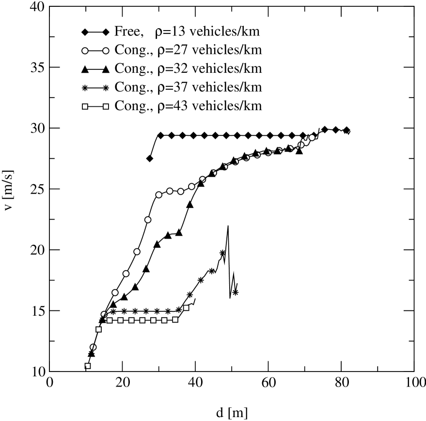
FIG. 29.: OV function in free flow and congested traffic of the KKW model for different densities. The same set of parameters as in Fig. 28 has been used.

Measurements of the OV-function show that the microscopic structure of the model differs from the empirical findings. In free flow traffic small headways are almost not observed and the maximum speed is reached at larger distances than in real traffic. This indicates that, compared to real traffic, the repulsive part of the car-car interactions is overemphasized. While the differences between empirical data and model results might be reduced for a different set of model parameters, the model results for synchronized traffic differ even qualitatively. In real traffic one observes for a given density a crossover from a density independent form of the OV-function at small distances to an asymptotic velocity for larger distances (see Fig. 4) which depends on the density. This is not reproduced by the KKW model, where a distance independent average velocity is observed only in a narrow range of spatial headways, if it is observed at all.

The comparison between empirical and simulation results of the time-headway distribution indicates that the model largely fails to reproduce the empirical results obtained for free flow traffic. This is, as discussed before, partly a results of the simplified setup we used for our simulations. A much better agreement would be obtained if we consider a realistic distribution of maximal velocities. But even in this case one is left with a problem. The lack of velocity-anticipation leads to a sharp cut-off of the time-headway distributions for times less than one unit of time, i.e. $1~{}\rm{s}$. Although the position of the cut-off can be tuned by varying the temporal discretization, it must be noted that this still does not lead to the right functional form, as the maximum of the time-headway distribution is located at the minimal observed time-headway. This again confirms necessity of velocity anticipation for the reproduction of the empirical findings at short time-headways.

Summarizing the CA model introduced by Kerner, Klenov and Wolf reveals three distinguishable traffic states, as observed in empirical studies. The reproduction of the empirical time-headway distribution and fundamental diagram is partly satisfying and could be easily improved by the introduction of velocity anticipation. The most important differences between empirical findings and model results concern the OV-function. This indicates that the microscopic structure of the model states does not match the real structure of highway traffic. We also believe that this disagreement is due to the very nature of the car-car interactions in the KKW model and cannot be resolved by a better choice of the model parameters.

VII Comparison of the fundamental diagrams

The comparison of the models presented so far is based on local measurements of inductive loops. Therefore, the model parameters have been chosen in order to allow the best possible accordance with the empirical setup. One of the main disadvantages of local measurements is that the detected values of the flow and the velocity strongly fluctuate whereas density cannot even be defined locally in a strict sense. However, in traffic flow simulations it is possible to get averaged quantities that are representative for a given density. Therefore, in this section global measurements of the flow and the density of the various models are given for a typical set of parameters in order to demonstrate the characteristics of the approaches. However, since density can be calculated exactly, the distinction between the traffic states is omitted.

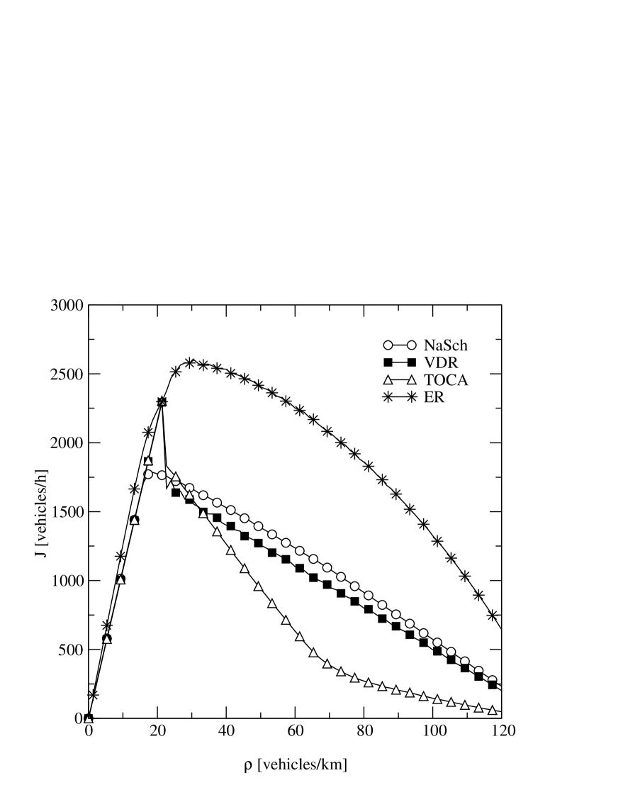
FIG. 30.: Comparison of the global fundamental diagram of the NaSch model, the VDR model, the TOCA, and the ER model for typical parameter values and a homogeneous initialization.

Density, flow and velocity can be measured globally in the following way: The density $\rho_{\rm{global}}$ can directly be obtained by counting the number $N$ of vehicles on a highway section of length $L$ via

$$\rho_{\rm{global}}=\frac{N}{L}.$$ (19)

The average velocity $v_{global}$ is then defined as

$$v_{\rm{global}}=\frac{1}{N}\sum_{n=1}^{N}v_{n}$$ (20)

with the velocity $v_{n}$ of vehicle $n$. Again, the hydrodynamical relation allows the calculation of the flow

$$J_{\rm{global}}=\rho_{\rm{global}}v_{\rm{global}}=\frac{1}{L}\sum_{n=1}^{N}v_{n}.$$ (21)

A typical fundamental diagram consists of a linear free flow branch that intersects with an almost linear congested branch. As one can see in Fig. 30 and Fig. 31 nearly all discussed models are able to reproduce this basic characteristics. The fundamental diagram of the HS model, however, exhibits two distinct maxima. The first maximum is simply given by the transition from free flow to congested traffic. The second maximum is a consequence of the chosen OV-curve. Since vehicles with $3\leq d\leq 5$ have to drive with a velocity of $2$, the flow increases linearly for densities well above a certain density until the average gap is smaller than $3$ cells. Moreover, due to the OV-curve the vehicles behave deterministically and choose their velocity according to the gap, i.e. $v=d$. As a result of a nearly uniform gap distribution, effectively speed limits are applied for certain density intervals which are reflected by the occurrence of different slopes in the congested branch of the fundamental diagram.

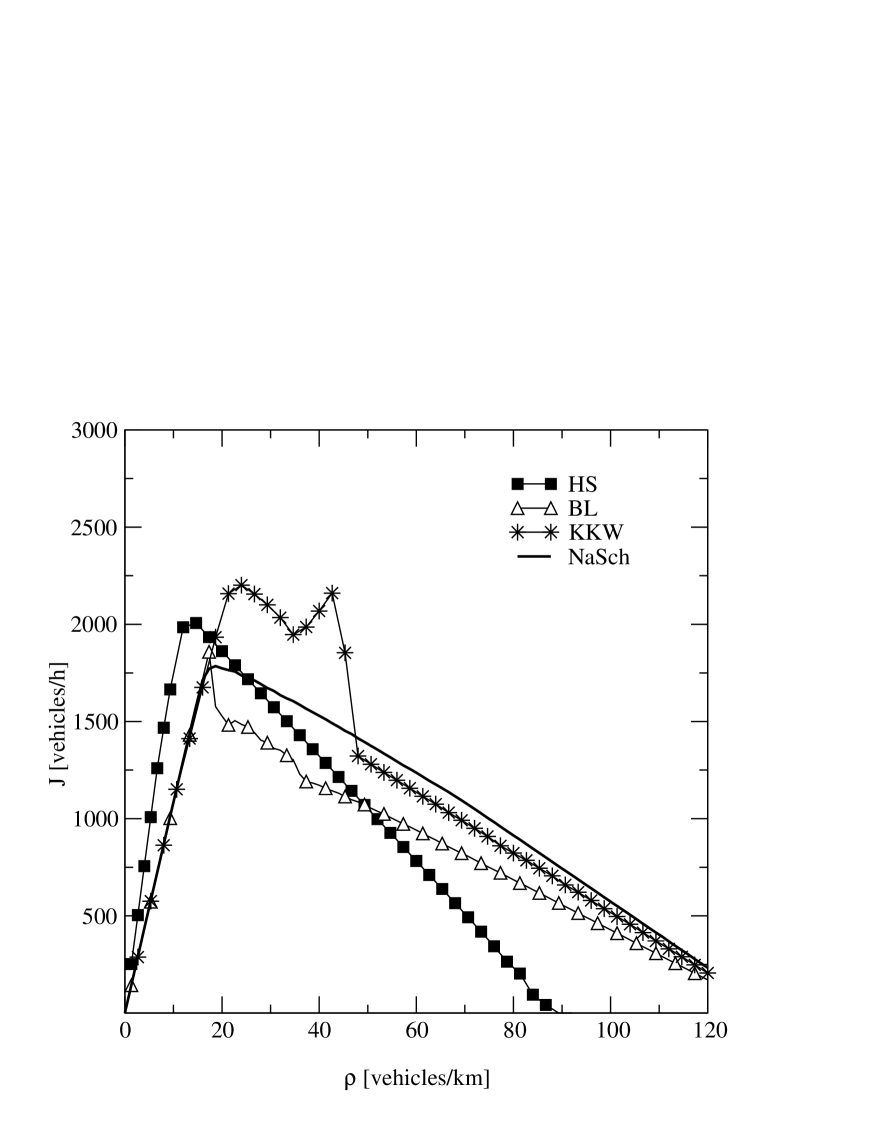
FIG. 31.: Comparison of the global fundamental diagrams of the HS model, the BL model, and the KKW model with that of the NaSch model for typical parameter values and a homogeneous initialization.

This behavior is typical for models with modified distance rules and can also be found in the ER model. Since the choice of the gap-velocity matrix in the ER model leads to speed limits for different density regimes, the free flow branch shows two different slopes like in the local measurements. Even more severe is the lack of a distinct maximum in the fundamental diagram. This is a consequence of the ordered sequential update of the ER model. It is possible that jams can also move in downstream direction, thus leading to many small jams with a large flow.

Measurements of empirical data have revealed that the outflow from a jam is reduced considerably compared to the maximum possible flow. As a result, metastable free flow states exist and hysteresis effects can be observed in the fundamental diagram [57].

Obviously, this is the case for the VDR model, the TOCA model as well as for the BL and KKW models while the maximum possible flow of the NaSch model is as large as the outflow from a jam.

Since the deceleration probability in the VDR model was chosen very small ($p_{{\rm dec}}=0.01$) the stability of the homogeneous branch of the fundamental diagram is very large. In contrast, once a jam has formed above a certain threshold density the large deceleration probability for the vehicles at rest is responsible for the reduced outflow from a jam. As a result, the system is phase separated into a region of free flow and a compact moving jam. The capacity drop can simply be tuned by varying the difference between the two deceleration parameters. In analogy to the VDR model, in the TOCA model only vehicles with $v\leq d$ decelerate with the probability $p$. Thus, vehicles driving with $v_{\rm{max}}$ and $d>v$ lead to a stable high flow branch in the fundamental diagram up to a density of $\frac{1}{v_{\rm{max}}+1}$. However, the congested regime of the TOCA model reveals the existence of two different slopes in the fundamental diagram. For densities larger than $1/2$ vehicles have on average a gap of less than one cell. Since the vehicles decelerate with a large probability, but do accelerate with a rate smaller than one, the system now contains only one large jam whose width is comparable to the system size.

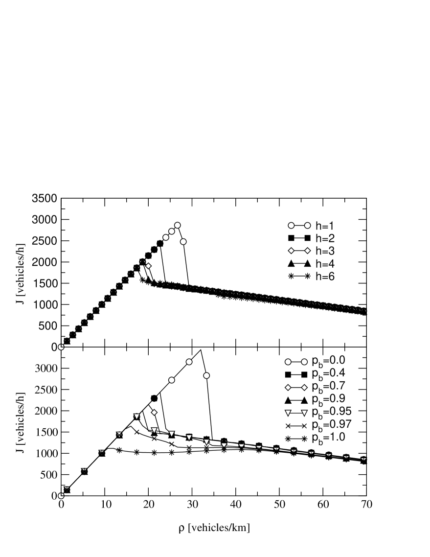
FIG. 32.: Fundamental diagram for different horizons $h$ (top) and for different $p_{b}$ (bottom). All simulations have been performed with an homogeneous initialization.

Like in the VDR model, in the BL model the high flow states can simply be controlled by the deceleration parameter $p_{0}$ for vehicles at rest. However, in the congested regime two distinct slopes of the fundamental diagram become visible. The density at which the slope changes and the shape of the fundamental diagram can be triggered by the parameters $h$ and $p_{b}$ that determine the interaction between vehicles with $d>v$. In particular, the higher $h$ the smaller the density $\rho_{\rm{max}}$ of the maximum flow (Fig. 32 top). For large $h$ the fundamental diagram converges very fast, so that the fundamental diagram for values larger than $h=8$ are identical. Moreover, even small values of $p_{b}$ have a strong influence on the flow. The high flow branch of the fundamental diagram (Fig. 32 bottom) and the density $\rho_{\rm{max}}$ of maximum flow are reduced. For large values the congested branch of the fundamental diagram shows two different slopes. The higher $p_{b}$, the smaller the density at which the slope changes.

A Minimal model?

The BL model improves, compared to the other models we discussed in this work, the agreement with the empirical data, especially in the case of the OV-curve. Nevertheless, this is only possible with the application of a variety of new update rules. Therefore, it remains an open question whether this set of update rules can be reduced.

In the top part of Fig. 33 we successively dropped the extensions of the model. First, the slow-to-start rule has been omitted. Without the slow-to-start rule the model lacks the ability of a reduced outflow from a jam and the number of large compact jams is reduced so that the flow increases. As a further reduction of the model, anticipation is switched off. This leads to a decrement of the flow at densities larger than the density of maximum flow. Now headways smaller than the velocity are not possible, which manifests in the OV-curve at small densities. For large densities the anticipation of the predecessors velocity becomes more and more difficult until anticipation is no longer applicable. Therefore, the differences between the curves with and without anticipation vanishes.

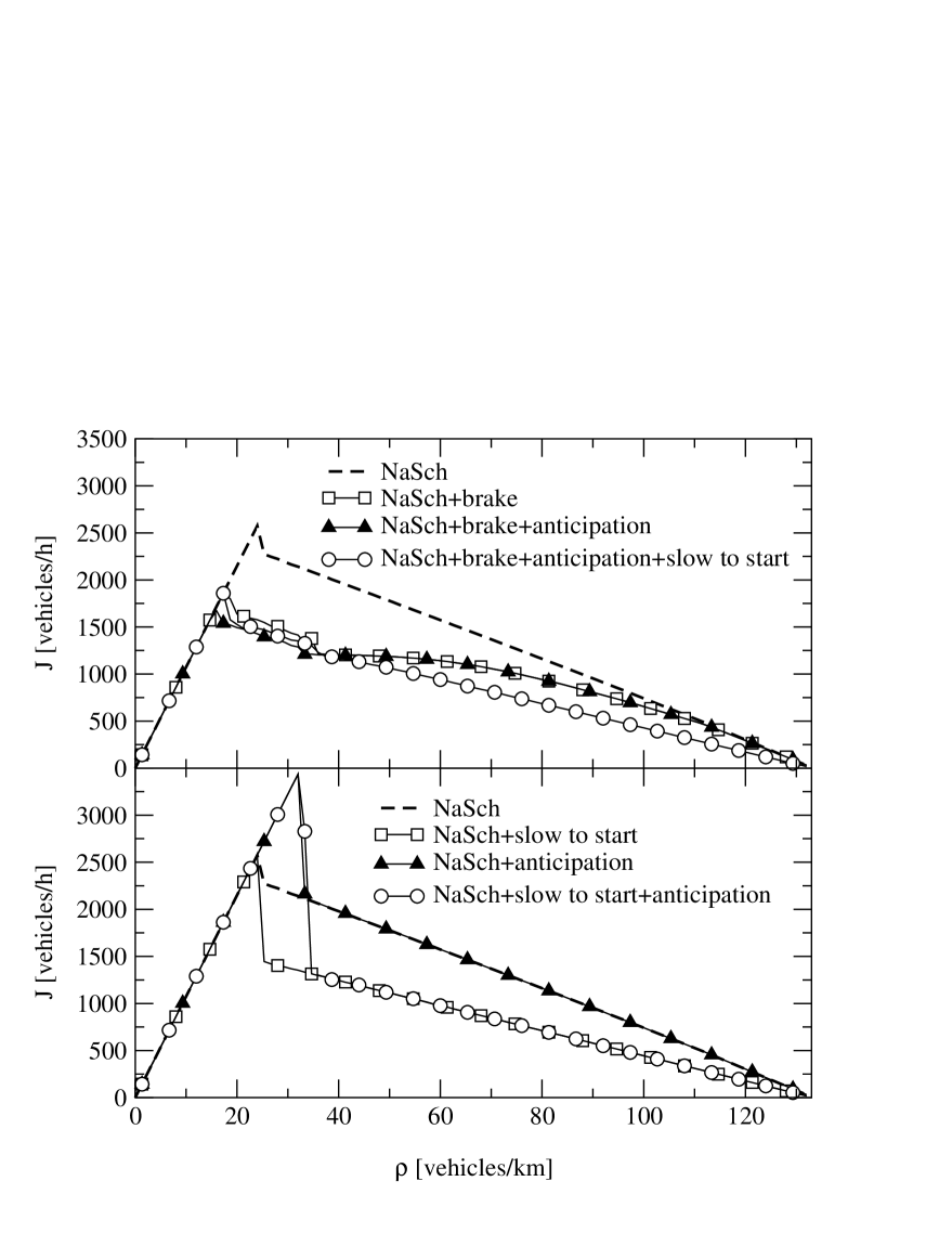
FIG. 33.: Successive extension of the NaSch model with brake lights (top) and without brake lights (bottom). Note that the system is initialized in an homogeneous state to generate also high flow states.

Applying the braking rule as the only extension leads to a plateau-like fundamental diagram compared to the NaSch model. Additionally, the flow is reduced dramatically. It is the brake rule that changes the shape of the fundamental diagram.

In bottom part of Fig. 33 the same successive reductions of the rules have been applied to the model without braking rule. Neither the anticipation, nor the slow-to-start rule applied as a single extension or in combination are able to change the shape of the fundamental diagram.

Considering the empirical fact that small time-headways and a reduced outflow from a jam exist, the braking rule is the only new extension of the NaSch model. This new rule turns out to be crucial for the correct generation of the OV-curves and the occurrence of synchronized traffic.

So the set of rules chosen for the BL model is minimal in the sense that all are needed to obtain a satisfactory agreement with empirical data. We also believe that is essential to combine car-following like behavior and distance based rules. In case of the BL-model the velocity adjustment is event driven, i.e. the drivers react to braking cars in the upstream flow. It is not excluded that the same can be achieved with a different, but simpler set of rules. This is highly desirable in order to reduce the complexity of the model and the number of parameters. However, it is currently unclear whether there is a similarly simple physical mechanism behind the formation of synchronized traffic as it is behind the formation of wide jams. For the latter, the reduction of the outflow from a jam below the maximal flow is essential which can be easily achieved by any kind of slow-to-start rule.

VIII Discussion

The intention of our investigation was to single out the models which are able to describe the empirically observed microscopic structure of traffic flow correctly. It is well-known that many quite different models exist which reproduce the macroscopic properties (e.g. global fundamental diagrams or spontaneous jam formation) rather accurately [1, 2, 3]. However, recently single-vehicle data have become available. A thorough analysis of these data has allowed for a deeper understanding of the microscopic properties which now should be incorporated into the different modeling approaches.

We have suggested a test scenario based on the comparison of computer simulations in a realistic setup with empirical data obtained using stationary inductive loops. An important point is that we have used only one fixed set of model parameters which has been determined by comparison with empirical data, e.g. with the free-flow velocity. Therefore we are able to determine whether a model is able to describe all traffic situations consistently without the necessity to tune parameters according to the state.

Our focus was on cellular automata models [1] and especially variants of the Nagel-Schreckenberg model [10, 11] which can be considered as a minimal CA model for traffic flow. Our comparison has revealed differences between the models on a macroscopic scale which become even more pronounced on a microscopic level of description.

We have seen that models with modified distance rules, like the ER and the HS model, have problems on a macroscopic level. They are not able to produce a realistic (global) fundamental diagram and it is difficult to make these models intrinsically crash-free.

The NaSch model, the VDR model, the TOCA model and the brake light version of the NaSch model reproduce the fundamental diagram quite well. This is already sufficient for many applications. In urban traffic, for example, the dynamics of the vehicles between two intersections is predominantly determined by traffic lights. The correct description of queues at cross-roads, therefore, only requires the existence of two distinct traffic phases, namely free flow and congested traffic.

More realistic applications of traffic flow simulations, e.g., that allow the tracing of a jam, need a more detailed description of the jamming mechanisms. For the correct reproduction of the upstream propagation of the downstream front of a jam it is necessary to reduce the outflow from a jam and thus to facilitate metastable states. Here, the VDR model, the TOCA model and the BL model allow the existence of states with a flow considerably larger than the outflow from a jam.

Differences between the models can be observed in the jam dynamics. While the road in the VDR model is separated into a region with free flow and a compact jam that propagates upstream, the peculiarities of the update rules of the TOCA model lead to a jam that covers the whole system.

Large compact jams appear also in the BL model since the slow-to-start rule of the VDR-model is included. However, brake lights are responsible for the generation of synchronized regions, i.e., regions of vehicles that are moving with a small velocity but high flow.

This difference in the vehicle dynamics becomes most obvious in the analysis of locally measured single-vehicle data. On a microscopic level of description the main difficulty lies in the reproduction of small time-headways that can be found at low densities in free flow and in the density dependence of the velocity-distance relationship. This important behavior of the OV-curve demonstrates that the driving strategy of a vehicle depends strongly on the traffic state while the vehicles in most modeling approaches adjust their velocity directly according to their headway only, and therefore by the density.

As a first step towards a realistic modeling of highway traffic the interaction horizon of the original NaSch model has be to enhanced like in the TOCA, the ER and the HS model. However, in the TOCA and the HS model the cell length is not decreased which is necessary in order to reproduce realistic acceleration values. Therefore, the benefits of the increased interaction horizon do not become visible. Moreover, vehicles do react in a static manner to a stimulus within the horizon. In particular, the velocity gap matrix used in the ER model just leads to speed limits for certain densities.

A further step is the incorporation of the idea of event-driven anticipation. In contrast to the static reaction described in the previous paragraph it allows for a dynamical response that will enable the vehicles to adjust their velocity to the actual traffic situation regardless of the traffic density in front. This idea is realized in the BL and KKW models. It turns out, that in case of the BL model only the introduction of brake lights, which allow the timely adjustment of the velocity to the downstream speed and can propagate in upstream direction, allows the reproduction of synchronized traffic. Of course, there might alternative ways to model synchronized traffic, but we believe that long-ranged event-driven interactions between the vehicles are essential.

The use of an effective gap by means of velocity anticipation reduces velocity fluctuations in free flow and leads to platoons of vehicles driving bumper-to-bumper. It is also worth mentioning that this effect is of special importance in multi-lane traffic as shown in [47].

We have seen that the BL model allows to overcome the problems in the reproduction of synchronized traffic encountered in the other modeling approaches. It reproduces qualitatively the observed behavior. Even the quantitative agreement is in most cases very good although the test scenario has neglected effects like disorder (different vehicle and driver types) and boundary conditions. In contrast, in most other approaches the discrepancies between empirics and model behavior can already be seen on a qualitative level. In particular, in the simulations of the BL model three qualitatively different microscopic traffic states are observed in accordance with the empirical results. The deviations of the simulation results are mainly due to simple discretization artifacts which do not reduce the reliability of the simulation results. We also want to stress the fact that the agreement is on a microscopic level. This improved realism of the BL model leads to a larger complexity of the approach compared to other models of this type. Nevertheless, due to the discreteness and the local car-car interactions, very efficient implementations should still be possible. Moreover, the adjustable parameter of the model can be directly related to empirical quantities. The detailed description of the microscopic dynamics will also lead to a better agreement of simulations with respect to empirical data for macroscopic quantities, e.g., jam-size distributions. Therefore we believe that this approach should allow for more realistic micro-simulations of highway networks.

Our results show that the CA models for highway traffic have reached a very high degree of realism. The most complete description of the empirical findings is by means of the BL model. This is not surprising since the model has been designed in order to reproduce data of local measurements. But anyhow it is important to know which aspects of real traffic are described by a certain model, because in the end the aspired accordance of a model with empirical observations strongly depends on the goal of the particular application. So it is useful to use oversimplified model approaches in order to concentrate on particular aspects of traffic flow phenomena [60].

Finally we want to emphasize that the results obtained from modelling approaches also help to improve our understanding of the general principles of traffic flow. We have seen the the complexity of human behavior becomes more important if one wants to reproduce its properties more accurately. In the simplest case only the accident-avoidence is sufficient to reproduce the basic properties, like free-flow and jammed phases. For synchronized traffic, however, this is not sufficient. Here the results indicate that the dependence of the driving-strategy on the traffic state becomes essential. Drivers do not only want to avoid crashes, but also drive comfortably, e.g. by avoiding unnecessary large acceleration or deceleration. This has been emphasized in [20] and is implemented in slightly different form in the BL and KKW models.

The next step would be the inclusion of other modelling approaches, not only cellular automata models. Using a different test scenario this has recently been done by Brockfeld and Wagner [70]. They have compared travel-time for various models (e.g. NaSch, VDR and OVM) with empirical data. Using methods from optimization theory to determine the best parameters it was surprisingly found that all models produce similar results that are not in good agreement with the data. The reason for this is not understood. However, the performance of more sophisticated models (like BL and KKW) has not been investigated in [70].

Acknowledgement:

The authors have benefited from discussions with R. Barlović, S. Grabolus, D. Helbing, T. Huisinga, L. Neubert, C. Rössel, and D.E. Wolf. L. Santen acknowledges support from the Deutsche Forschungsgemeinschaft under Grant No. SA864/2-1. We also thank the Ministry of Economics and Small Businesses, Technology and Transport of North-Rhine Westfalia as well as to the Federal Ministry of Education and Research of Germany for financial support (the latter within the BMBF project “SANDY”).

A Continuous limit of the NaSch model

The adjustment of the acceleration of the vehicles in the original NaSch model to empirical values (that are about $1~{}m/s^{2}$ [50]) requires the decrement of the length of a cell (see also [13, 61, 62]).

FIG. 34.: NaSch model with different $v_{\text{max}}$ and homogeneous initialization.

This, however, entails an increment of the maximum possible velocity for a given fixed absolute value of $v_{\text{max}}$ (about $100~{}km/h$ throughout this paper).

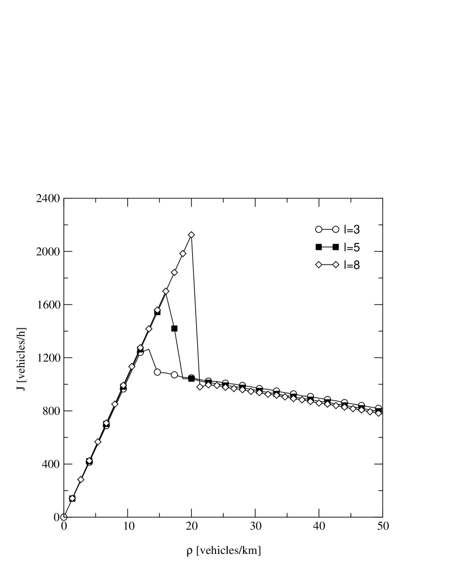
FIG. 35.: Fundamental diagram of the NaSch model with $p_{\rm{dec}}=0.5$ for different discretizations and homogeneous initialization.

It turns out, that already the increment of the number of states a vehicle is allowed to adopt leads to hysteresis effects of the flow. In particular, the flow can be enhanced in a certain density regime by initializing homogeneously the vehicles on the lattice compared to a pure random initial setup. As a result, in the limit $v_{\text{max}}\rightarrow\infty$ [63, 64, 61, 62] the system exhibits metastable states (Fig. 34) with a flow increasing proportional to $v_{\text{max}}$, but with a rapidly decreasing lifetime.

Unfortunately, increasing only $v_{\text{max}}$ leads to a significant decrement of the density of maximum flow. Thus, in order to keep the maximum velocity fixed, the limit $v_{\text{max}}\rightarrow\infty$ with $v_{\text{max}}/l=$ const. with the length $l$ of a cell has to be considered. Fig. 35 shows fundamental diagrams for different finer discretization. Since the acceleration step of a vehicle is decreased considerably, velocity fluctuations and vehicle interactions in free flow are reduced. A random initialization of the system does not allow the high flow states so that hysteresis can be observed. On one hand, with increasing deceleration probability $p_{\rm{dec}}$ the stability of the homogeneous flow branch of the fundamental diagram decreases, but on the other hand the capacity drop increases.

Unlike in the VDR model, the origin of the high flow states cannot be traced back to a reduction of the outflow from a jam but to the stability of the free flow state.

A system with length $l$ and deceleration probability $p_{\rm{dec}}$ behaves like a NaSch model with cell length $1$ and a considerably smaller deceleration probability of about $p_{\rm{dec}}/l$. In contrast, in the congested regime the influence of the cell length can be neglected and a system with decreased cell length behaves analogously to the NaSch model with the same deceleration probability, e.g., the dynamics of the vehicles in the congested regime of the NaSch model is maintained (unlike in the cruise control limit of the NaSch model [65] where cars that are driving with $v_{\text{max}}$ have a deceleration probability $p_{\rm{dec}}(v_{\text{max}})=0$).

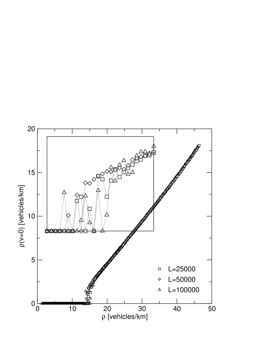
FIG. 36.: Order-parameter $\eta$ for the NaSch model with a cell length of $1.5$ m and different system sizes $L$ for $p_{\rm{dec}}=0.5$ and a homogeneous initialization. The inset zooms into the transition region.

For realistic traffic simulations it is important that the high flow states are metastable for finite systems in the sense that the probability for a perturbation that leads to a collapse of the flow is only very small. Nevertheless, in the thermodynamic limit the high flow states become unstable so that the homogeneous branch of the fundamental diagram vanishes.

In order to study the phase transition we introduced an order parameter that exhibits a qualitatively different behavior within the two phases. Because of the mass conservation in the NaSch model with periodic boundary conditions we observed the density $\eta$ of jammed cars:

$$\eta=\frac{1}{L}\sum_{i=1}^{N}\delta_{v_{i},0}.$$ (A1)

In the NaSch model $\eta$ decays exponentially in the vicinity of the transition [66] whereas a sharp drop occurs in the VDR model [67]. Due to the finite braking probability in the NaSch model cars with zero velocity do exist even at densities below the transition density. In contrast, due to the small deceleration probability $p_{\rm{dec}}$ in the VDR model one macroscopic jam forms only at densities above the transition density. With increasing $p_{\rm{dec}}$ the transition smears out.

Analogously to the VDR model, the order parameter of the NaSch model with a finer discretization (Fig. 36) shows a transition from zero to a linear dependence of the density. With increasing system size the high-flow states become unstable and the jump in the order parameter vanishes which demonstrates the metastability of the high flow states.

B Accidents in the HS-model: A static criterion

In order to ensure collision-free motion in a model with parallel update the condition

$$v_{n}(t+1)\leq d_{n}-1+v_{n+1}(t+1)$$ (B1)

must always be fulfilled, i.e., the new velocity $v_{n}(t+1)$ of a car has to be smaller than the number $d_{n}-1$ of empty cells in front plus the number $v_{n+1}(t+1)$ of cells the preceding car moves in the next time-step. Eqn. (B1) has to be complemented by the inequality $0\leq v_{n}(t+1)$ that ensures that vehicles do not move backwards.

Consider now the case where the vehicle approaches the end of a jam, i.e., the preceding car is standing and will not move in the next time-step ($v_{n+1}(t+1)=0$). Using the acceleration rule eqn. (4), condition eqn. (B1) can be rewritten as

$$v_{n}(t+1)+\Big{\lfloor}\lambda[V_{\rm{opt}}(d_{n})-v_{n}(t+1)]\Big{\rfloor}\leq d_{n}-1.$$ (B2)

In order to be intrinsically free of collisions, condition (B2) has to be satisfied for all $d$ and all $v$. For $\lambda=1$ the inequality (B2) is always satisfied if $V_{\rm{opt}}(d_{n})\leq d_{n}-1$. For general $\lambda$, however, this is not the case.

This can easily be verified by initializing the system in a compact jam. In our simulations jams always occurred for global densities larger than $20$ veh/km when the first car arrived at the jam. This simulation result has to be discussed in the context of the empirical results of the jam dynamics. Empirically one observes quite often a jam surrounded by free flow traffic. This includes the fact that cars approach the upstream front of jams with a rather large velocity. Unfortunately for the HS model these kind of configurations lead to accidents, which is in sharp contrast to the real situation.

But how does one have to choose $\lambda$ for a given OV function? Using the inequalities $x\geq\lfloor x\rfloor>x-1$ (for $x<0$) one can derive sufficient conditions on the sensitivity parameter $\lambda$ for the model to be realistic in the sense that no collisions occur

$$\lambda>\max\left\{\frac{d-v-1}{V_{\rm{opt}}(d)-v}:v>V_{\rm{opt}}(d)\right\},$$ (B3)

and vehicles do not move backwards

$$\lambda\leq\min\left\{\frac{v}{v-V_{\rm{opt}}(d)}:v>V_{\rm{opt}}(d)\right\}.$$ (B4)

We checked these two conditions for the OV-function given in [18]. It turns out that for the chosen $V_{\rm{opt}}$-function $\lambda=1$ is the only possible choice. The upper limit for $\lambda$ holds for a quite general class of OV-functions, i.e., it is the upper limit for all OV-functions having $V_{\rm{opt}}=0$ for some value of the gap.

REFERENCES

- [1] D. Chowdhury, L. Santen, and A. Schadschneider, Physics Reports 329, 199 (2000) and Curr. Sci. 77, 411 (1999).
- [2] D. Helbing, Rev. Mod. Phys. 73, 1067 (2001).
- [3] T. Nagatani, Rep. Prog. Phys. 65, 1331 (2002).
- [4] K. Nagel, P. Wagner, R. Woesler, Oper. Res. 51, 681 (2003)
- [5] R. Herman and K. Gardels, Sci. Am. 209 (6), 35 (1963).
- [6] D.C. Gazis, R. Herman, and R.W. Rothery, Op. Res. 9, 454 (1961).
- [7] D.C. Gazis, Science 157, 273 (1967).
- [8] P.G. Gipps, Transp. Res. 15B, 105 (1981).
- [9] R.W. Rothery, in: N. Gartner, C.J. Messner, A.J. Rathi (eds.), Transportation Research Board (TRB), Special Report 165, Traffic Flow Theory, 2nd ed. (1998).
- [10] K. Nagel and M. Schreckenberg, J. Physique I 2, 2221 (1992).
- [11] M. Schreckenberg, A. Schadschneider, K. Nagel, and N. Ito, Phys. Rev. E 51, 2939 (1995).
- [12] J. Esser and M. Schreckenberg, Int. J. Mod. Phys. C8, 1025 (1997).
- [13] S. Krauss, P. Wagner and C. Gawron, Phys. Rev. E 54, 3707 (1996), and 55, 5597 (1997)
- [14] D.E. Wolf, Physica A 263, 438 (1999).
- [15] R. Barlovic, L. Santen, A. Schadschneider, and M. Schreckenberg, Eur. Phys. J. B5, 793 (1998).
- [16] W. Brilon and N. Wu (1999), in Traffic and Mobility ed. W. Brilon, F. Huber, M. Schreckenberg, and H. Wallentowitz (Berlin: Springer)
- [17] H. Emmerich and E. Rank, Physica A 234, 676 (1997).
- [18] D. Helbing and M. Schreckenberg, Phys. Rev. E 59, R2505 (1999).
- [19] W. Knospe, L. Santen, A. Schadschneider, and M. Schreckenberg, J. Phys. A33, L477 (2000).
- [20] W. Knospe, L. Santen, A. Schadschneider, and M. Schreckenberg, Phys. Rev. E 65, 015101 (2002).
- [21] B.S. Kerner, S.L. Klenov, and D.E. Wolf, J. Phys. A35, 9971 (2002).
- [22] L. Neubert, L. Santen, A. Schadschneider, and M. Schreckenberg, Phys. Rev. E 60, 6480 (1999).
- [23] B. Tilch and D. Helbing, In: Traffic and Granular Flow ’99, p. 333, D. Helbing, H. J. Herrmann, M. Schreckenberg, D. E. Wolf (eds.) Springer (Heidelberg, 2000).
- [24] W. Knospe, L. Santen, A. Schadschneider, and M. Schreckenberg, Phys. Rev. E 65, 056133 (2002).
- [25] I.A. Lubashevsky, R. Mahnke, P. Wagner, and S. Kalenkov, Phys. Rev. E 66, 016117 (2002).
- [26] B.S. Kerner, Netw. Spatial Econo. 1, 35 (2001)
- [27] D. Helbing, M. Treiber, Coop. Tr@nsp. Dyn. 1, paper 2 (2002)
- [28] F. L. Hall, B. L. Allen,and M. A. Gunter, Transp. Res. A 20A, 197 (1986).
- [29] B. S. Kerner, Phys. World 8, 25 (1999).
- [30] L. Neubert, Statistische Analyse von Verkehrsdaten und die Modellierung von Verkehrsfluss mittels zellularer Automaten, Ph.D. thesis, University Duisburg (2000).
- [31] B.S. Kerner, Phys. Rev. Lett. 81, 3797 (1998).
- [32] B.S. Kerner and H. Rehborn, Phys. Rev. E 53, R1297 (1996).
- [33] M. Bando and K. Hasebe, A. Nakayama, A. Shibata, and Y. Sugiyama, Phys. Rev. E 51 1035 (1995).
- [34] M. Fukui and Y. Ishibashi, Phys. Rev. E 51, 2339 (1995).
- [35] K. Nishinari and D. Takahashi, J. Phys. A 32, 93 (1999)
- [36] G.M. Schütz, in: Phase Transitions and Critical Phenomena, Vol.19, eds. C. Domb and J.L. Lebowitz (Academic Press, 2000)
- [37] K. Ghosh, A. Majumdar, and D. Chowdhury, Phys. Rev. E 58, 4012 (1998).
- [38] A. Schadschneider and M. Schreckenberg, Ann. Physik 6, 541 (1997).
- [39] M. Takayasu and H. Takayasu, Fractals 1, 860 (1993).
- [40] C. Appert, L. Santen, Phys. Rev. Lett. 86, 2498 (2001)
- [41] R. Barlovic, T. Huisinga, A. Schadschneider, and M. Schreckenberg, Phys. Rev. E 66, 046113 (2002).
- [42] B.S. Kerner and P. Konhäuser: Phys. Rev. E 48, R2335 (1993).
- [43] N. Rajewsky, L. Santen, A. Schadschneider, and M. Schreckenberg, J. Stat. Phys. 92, 151 (1998).
- [44] D. Helbing and B. Tilch, Phys. Rev. E 58, 133 (1998).
- [45] A. Sasoh, J. Phys. Soc. Jpn. 70, 3161 (2001).
- [46] C. L. Barrett, and M. Wolinsky, in Traffic and Granular Flow ed. D. E. Wolf, M. Schreckenberg and A. Bachem (Singapore: World Scientific), p.169.
- [47] W. Knospe, L. Santen, A. Schadschneider, and M. Schreckenberg, Physica A 265, 614 (1999).
- [48] M. Goldbach, A. Eidmann, and A. Kittel, Phys. Rev. E 61, R1239 (2000).
- [49] R. Herman and R.W. Rothery, Car Following and Steady-State Flow, Proceedings of the 2nd International Symposium on the Theory of Traffic Flow, Ed. W. Leutzbach and P. Baron, Bonn, Germany, 1965.
- [50] Institute of Transportation Engineers (1992). Traffic Engineering Handbook, Washington, DC.
- [51] H.P. George, Measurement and Evaluation of Traffic Congestion, Bureau of Highway Traffic, Yale University 1961, 43-68.
- [52] A.J. Miller, Jrl. Roy. Statist. Soc. B 23 (1961) 1.
- [53] J. Schlums, Untersuchungen des Verkehrsablaufes auf Landstraßen, Eigenverlag, Hannover (1955).
- [54] Highway Capacity Manual, U.S. Department of Commerce, Bureau of Public Roads, Washington D.C. 1965, HRB Spec. Rep. 87 (1965)
- [55] L.C. Edie and R.S. Foote, Proc. HRB 37, 334 (1958).
- [56] R.C. Pfefer, Transportation Engineering Journal of American Society of Civil Engineers, Vol. 102, No. TE4, 683-697 (November 1976).
- [57] B.S. Kerner and H. Rehborn, Phys. Rev. Lett. 79, 4030 (1997).
- [58] B.S. Kerner and S.L. Klenov, J. Phys. A35, L31 (2002).
- [59] B.S. Kerner and S.L. Klenov, Phys. Rev. E 68, 036130 (2003).
- [60] K. Nagel, Phys. Rev. E 53 (5), 4655.
- [61] S. Grabolus, Numerische Untersuchungen zum Nagel-Schreckenberg-Verkehrsmodell und dessen Varianten, Diplomarbeit, Universität zu Köln, Germany (2001).
- [62] S. Grabolus and A. Schadschneider, in preparation.
- [63] M. Sasvári and J. Kertész, Phys. Rev. E 56, 4104 (1997).
- [64] Ding-wei Huang and Chung-wei Tsai, Phys. Rev. E 61, 012101 (2001).
- [65] K. Nagel and M. Paczuski, Phys. Rev. E 51, 2909 (1995).
- [66] B. Eisenblätter, L. Santen, A. Schadschneider, and M. Schreckenberg, Phys. Rev. E 57, 2 (1998).
- [67] G. Diedrich, Numerische Untersuchung zur Phasenseparation in Zellularautomaten für Strassenverkehr, Diplomarbeit, Universität zu Köln, Germany (1999).
- [68] R. Jiang and Q.-S. Wu, J. Phys. A 36, 381 (2003)
- [69] M. Krbalek and D. Helbing, Physica A333, 370 (2004)
- [70] E. Brockfeld and P. Wagner, in Interface and Transport Dynamics — Computational Modelling, edited by H. Emmerich, B. Nestler, M. Schreckenberg (Springer 2003)