Fluctuation conductivity of thin films and nanowires near a parallel-field-tuned superconducting quantum phase transition

Abstract

We calculate the fluctuation correction to the normal state conductivity in the vicinity of a quantum phase transition from a superconducting to normal state, induced by applying a magnetic field parallel to a dirty thin film or a nanowire with thickness smaller than the superconducting coherence length. We find that at zero temperature, where the correction comes purely from quantum fluctuations, the positive “Aslamazov-Larkin” contribution, the negative “density of states” contribution, and the “Maki-Thompson” interference contribution, are all of the same order and the total correction is negative. Further we show that based on how the quantum critical point is approached, there are three regimes that show different temperature and field dependencies which should be experimentally accessible.

The high interest in the physics of a quantum critical point (QCP) is motivated by the explosive growth of its experimental realizations, driving, in turn, a quest for theoretical understanding of quantum phase transitions (QPT)Sachdev_book . The challenge for theory is two fold: First, it is desirable to identify experimentally accessible systems experiencing QPT. Second, these systems should allow for a systematic and comprehensive theoretical description. In this respect, the QCP realized in dirty superconductors of reduced dimensionsGantmakher ; Liu01 under application of magnetic field represents an exemplarily controllable system allowing complete experimental exploration of the vicinity of the critical point on the one hand and systematic theoretical study on the other.

In this letter we present a full systematic investigation of fluctuation correctionsCraven73 ; LarkinV to the normal state conductivity of a thin wire or a thin film in the vicinity of a QPT from superconducting to normal state, induced by an applied magnetic field. We consider a thin wire (or thin film) of diameter $d$ (or thickness $t$ for the film) much smaller than the superconducting coherence length $\xi$. The magnetic field $H$ is applied along the wire (or parallel to the film) and can be parameterized completely by a scalar pair-breaking parameter Larkin65 (similar to the effect of paramagnetic impuritiesAbrikosov61 )

$$\alpha=\left\{\begin{array}[]{ccc}D\,(eHd/2c)^{2}/4&&\text{wire }\\ D\,(eHt/c)^{2}/6&&\text{film }\end{array}\right.$$ (1)

where $D$ is the diffusion coefficient in the bulk sample Zeeman . The superconducting critical temperature $T_{c}$ is related to $\alpha$ (see Fig. 1) via the standard equation

$$\ln(T_{c}/T_{c0})=\psi(1/2)-\psi(1/2+\alpha/2\pi T_{c}),$$ (2)

where $\psi$ is the digamma function and $T_{c0}\equiv T_{c}(H=0)$ is the critical temperature in the absence of a magnetic field. One can immediately see that at $T=0$ the superconductivity is destroyed at $\alpha_{c0}\equiv\alpha_{c}(T=0)=\pi T_{c0}/2\gamma$, where $\ln\gamma\approx 0.577$ is the Euler constant. Realization of the superconducting QCP in a superconductor with paramagnetic impurities was first suggested in the work of Ref.RamazashviliC97 (see also Ref.MineevS01 ). Since in our case the depairing parameter $\alpha$ depends on $H$, it allows for a well controlled exploration of the QPT and its vicinity by varying the applied magnetic field.

Figure 1: Phase diagram of a superconducting nanowire (thin film) in a parallel magnetic field (parametrized by $\alpha$). The boundary between the quantum and the intermediate regime, shown by a dotted line is different for a wire and film as marked in the figure while all other boundaries coincide.

Our main result for the fluctuation correction to the normal state conductivity can be presented as

$$\delta\sigma(\alpha,T)=\delta\sigma_{0}(\alpha)+\delta\sigma_{\scriptscriptstyle T}(\alpha,T),$$ (3)

where $\delta\sigma_{0}(\alpha)$ and $\delta\sigma_{T}(\alpha,T)$ are the zero temperature and finite temperature contributions, respectively. The zero temperature correction is given by

$$\delta\sigma_{0}(\alpha)=-{\frac{{2De^{2}}}{{\pi d(2+d)}}}\int{\frac{{d^{d}q}}{{(2\pi)^{d}}}}{\frac{{(Dq^{2})^{2}}}{{\alpha_{q}^{3}\,\ln(\alpha_{q}/\alpha_{c})}},}$$ (4)

where $\alpha_{q}\equiv\alpha+Dq^{2}/2$ and $d=1,2$ corresponds to a wire and film respectively. Its magnitude decreases monotonically with increasing field; this leads to a negative magnetoresistance. Note that a negative magnetoresistance was found also in granular superconductorsBeloborodov and in thin films in perpendicular magnetic fieldGalitskii01 . Shown in Fig.2 are plots of the dimensionless correction

$$\delta\bar{\sigma}_{0}(\alpha)=e^{-2}\times\left\{\begin{array}[]{cccc}(D/\alpha_{c0})^{-1/2}\,\delta\sigma_{0}(\alpha)&&&\text{wire}\\ \delta\sigma_{0}(\alpha)&&&\;\text{film.\; }\end{array}\right.$$ (5)

When expanded around the QCP, the dimensionless conductivity close to the QCP is given by

$$\delta\bar{\sigma}_{0}(\alpha)=\delta\bar{\sigma}_{0}(\alpha=\alpha_{c0})+\,b(\alpha-\alpha_{c0})/\alpha_{c0},$$ (6)

with the numerical coefficient $b=0.386$ and $b=0.070$ for a wire and film, respectively. Thus the zero temperature critical exponent is 1 for both $d=1,2$, at least within the perturbation theory.

In the vicinity of the QCP ($T,{\alpha-\alpha_{c}\ll}\alpha_{c0}$ ), the field dependence of $\delta\sigma_{T}(\alpha,T)$ turns out to be more singular than that of $\delta\sigma_{0}(\alpha)$ and for $T>\alpha-\alpha_{c}$ its leading term is given by

$$\delta\sigma_{\scriptscriptstyle T}(\alpha,T)=e^{2}\times\left\{\begin{array}[]{cccc}{\frac{{\sqrt{D}T}}{{4\sqrt{2}(\alpha-\alpha_{c})^{3/2}}}}&&&\text{wire}\\ {\frac{{T}}{{4\pi(\alpha-\alpha_{c})}}}&&&\text{film,}\end{array}\right.$$ (7)

while for $T<\alpha-\alpha_{c}$ it is

$$\delta\sigma_{\scriptscriptstyle T}(\alpha,T)=e^{2}\times\left\{\begin{array}[]{cccc}{\frac{{\pi\sqrt{D}T^{2}}}{{12\sqrt{2}(\alpha-\alpha_{c})^{5/2}}}}&&&\text{wire}\\ {\frac{{T^{2}}}{{18(\alpha-\alpha_{c})^{2}}}}&&&\text{film.}\end{array}\right.$$ (8)

The contributions $\delta\sigma_{\scriptscriptstyle T}$ and $\delta\sigma_{0}$ become comparable at

$$T\equiv T_{0}(\alpha)\sim\left\{\begin{array}[]{cccc}(\alpha-\alpha_{c0})^{7/4}/\,\alpha_{c0}^{3/4}&&&\text{wire}\\ (\alpha-\alpha_{c0})^{3/2}/\,\alpha_{c0}^{1/2}&&&\text{film.}\end{array}\right.$$ (9)

The key point is that the behavior of the fluctuation corrections to the conductivity depends on the way one approaches the QCP and we can identify three regimes in the vicinity of the QCP that show qualitatively different behaviors as illustrated in Fig. 1. There is a “classical” regime for $T>\alpha-\alpha_{c}$, where the correction is given by Eq.(7); an “intermediate” regime for $\alpha-\alpha_{c}>T>T_{0}(\alpha),$ where the correction behaves according to Eq.(8 ); and a “quantum” regime for $T_{0}(\alpha)>T$ where the behavior crosses over to an essentially zero-temperature-like behavior which is not singular and almost temperature independent with the fluctuation correction dominated by $\delta\sigma_{0}$ as given by Eqs.(4,5,6).

Figure 2: Dimensionless zero temperature fluctuation conductivity correction(5) as a function of depairing parameter $\alpha.$ Insert shows dependence of the resistivity on the magnetic filed for temperatures $T/\alpha_{c0}=0.01$ (upper curves) and $T/\alpha_{c0}=0.1$ (lower curves). Resistivity is normalized to the high temperature resistivity $R_{0}$ while the magnetic field is normalized to the critical filed $H_{c0}$ at $T=0.$

Since in the quantum region the correction to conductivity is negative whereas in the classical and intermediate region it is positive, we predict a non-monotonic behavior of the resistivity as a function of the magnetic field at finite temperature. The corresponding plots are shown in the insert of Fig. 2 for nanowires and thin films. Such behavior was indeed observed in experiments on amorphous thin filmsGantmakher , while for nanowires, to the best of our knowledge, it was not reported yet.

Our approach is based on the diagrammatic perturbation theory. Note that the technique using the time-dependent Ginzburg-Landau formalism that was adapted in Refs.RamazashviliC97 ; MineevS01 , accounts only for the direct “Aslamazov-Larkin” (AL) type of contributionAslamazovL68 to the fluctuation conductivity that comes from the charge transfer via fluctuating Cooper pairs, but misses the zero-temperature contribution to the correction. On the contrary, our approach, takes care of all the contributions including the “density of states” (DOS) part resulting from the reduction of the normal single-electron density of states at the Fermi level, and the more indirect “Maki-Thompson” (MT) interference contributionMaki68 ; Thompson70 . At zero temperature, where the correction comes purely from quantum fluctuations, these turn out to be of the same order as the AL contribution.

To derive our main results, we carry out a microscopic calculation within the standard framework of temperature diagrammatic technique in a disordered electron systemAGD ; AVR ; Altshuler80 in the diffusive limit (inverse mean free time $\tau^{-1}\gg T,\alpha$). Since we choose $d,t<\xi$ and parameterize the effect of field by $\alpha$ as defined by Eq.( 1), the problem effectively becomes one and two dimensional for a wire and film, respectively. The main building block of the diagrammatic technique in the presence of the BCS interaction is the so-called “Cooperon”, the ladder diagram that describes coherent scattering by impurities in the particle-particle channel. In the presence of a parallel magnetic field it is given by

$$C(\omega_{1},\omega_{2},q)={\frac{{2\pi\nu\theta(-\omega_{1}\omega_{2})}}{{|\omega_{1}-\omega_{2}|+Dq^{2}+2\alpha}}},$$ (10)

where ${\theta}$ is the step function, $\nu$ is the density of states at the Fermi surface, and $\mathbf{q}$ is the momentum in the effective dimension. Using Eq.(10) in a standard way, one obtains the “fluctuation propagator” i.e the impurity-averaged sum over the ladder diagrams corresponding to the electron-electron interaction in the Cooper channel,

$$K^{-1}(\Omega,q)=\ln\left({\frac{T}{{T_{c}^{0}}}}\right)-\psi\left({\frac{1}{2}}\right)+\psi\left({\frac{1}{2}}+{\frac{{\alpha_{q}+|\Omega|/2}}{{2\pi T}}}\right),$$ (11)

where $\Omega$ is the bosonic Matsubara frequency. The pole of Eq.(11) defines the boundary between the superconducting and normal phases given by Eq.(2). At low temperatures, $T\ll\alpha_{c0},$ the fluctuation propagator reduces to

$$K^{-1}(\Omega,q)=\ln[(\alpha_{q}+|\Omega)|/2)/\alpha_{c}(T)].$$ (12)

The fluctuation correction to the conductivity is obtained as usual from the Kubo formalism with the appropriate analytic continuation. The standard set of diagrams constituting the AL, DOS and MT contributions is shown in Fig. 3.

The AL contribution (Fig. 3a) can be expressed as a sum of two terms: $\delta\sigma^{AL}=\delta\sigma_{1}^{AL}+\delta\sigma_{2}^{AL}$ with

$${\frac{{\delta\sigma_{1}^{AL}}}{{e^{2}}}} = {\frac{{D^{2}}}{{2\pi Td}}}\int{\frac{{d^{d}q}}{{(2\pi)^{d}}}\frac{{d\Omega}}{{{\rm sh}^{2}{\frac{{\Omega}}{{2T}}}}}}\Bigl{[}\mathrm{Im}\{K(-i\Omega,q)\,\Gamma_{\Omega\mathbf{q}}^{2}\}$$

$$\times \mathrm{Im} \{K(-i\Omega,q)\}+\left(\mathrm{Im}\{K(-i\Omega,q)\,\Gamma_{\Omega\mathbf{q}}\}\right)^{2}\Bigr{]},$$ (13)

$$\vspace{0.2cm}{\frac{\delta{\sigma_{2}^{AL}}}{{e^{2}}}} = {\frac{{D^{2}i}}{{8\pi^{4}T^{3}}}}\int\frac{{d^{d}q\,d\Omega}}{{(2\pi)^{d}}}\;q_{x}^{2}\psi^{\prime}\left({\frac{1}{2}}+{\frac{\alpha_{q}-i\Omega/2}{{2\pi T}}}\right)$$ (14)

$$\times\psi^{\prime\prime}\left({\frac{1}{2}}+{\frac{\alpha_{q}{-i\Omega/2}}{{2\pi T}}}\right)K^{2}(-i\Omega,q),$$

where $\Gamma_{\Omega\mathbf{q}}\equiv(\mathbf{q}/2\pi T)\psi^{\prime}[1/2+(\alpha_{q}-i\Omega/2)/2\pi T].$ The contribution $\delta\sigma_{1}^{AL}$ appears only at finite temperature while $\delta{\sigma_{2}^{AL}}$ contains the contribution that survives even at $T=0$. Note that $\delta{\sigma_{2}^{AL}}$ that describes the quantum regime, results from differentiating $\Gamma_{\mathbf{q}}(-i\Omega)$ w.r.t $\Omega$ and is missed within the usual static approximation ( $\Omega=0$).

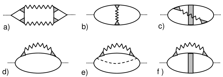
Figure 3: Diagrams for the fluctuation conductivity: a) Aslamazov-Larkin diagram, b)-c) Maki-Thompson diagrams, d)-e) density of states diagrams. Full line stands for the disorder averaged normal state Green’s function, wavy line for the fluctuation propagator $K$, the shaded rectangle for the Cooperon $C$ and shaded triangle for the vertex $C/2\pi\nu\tau$.

The MT correction is given by $\delta\sigma^{MT}=\delta\sigma_{1}^{MT}+\delta\sigma_{2}^{MT}$ where

$$\frac{{\delta\sigma_{1}^{MT}}}{{e^{2}}} = {\frac{{D}}{{2\pi}}}\int\frac{{d^{d}q\,d\omega d\Omega}}{{(2\pi)^{d}}}\text{th}{\frac{{\omega}}{{2T}}}K(-i\Omega,q)\left[{\frac{\text{cth}{{\frac{\Omega}{{2T}}}}}{{(\alpha_{q}-i\omega_{+})^{3}}}}\right.$$ (15)

$$\hskip 71.13188pt\left.+{\frac{{i}}{2T{\rm{sh}^{2}{\frac{{\Omega}}{{2T}}}}}\frac{{1}}{\alpha_{q}^{2}{+\omega_{+}^{2}}}}\right],$$

$$\frac{{\delta\sigma_{2}^{MT}}}{{e^{2}}} = -{\frac{{3D^{2}}}{{2\pi}}}\int\frac{{d^{d}q\,d\omega d\Omega}}{{(2\pi)^{d}}}\,{{\text{th}{\omega\over{2T}}}\over{\text{th}{\Omega\over{2T}}}}\,{{q_{x}^{2}K(-i\Omega,q)}\over{(\alpha_{q}-i\omega_{+})^{4}}},$$ (16)

with ${\omega_{+}\equiv\omega+\Omega/2}$. For low temperatures, the contributions $\delta\sigma_{1}^{MT}$ (Fig. 3b) and $\delta\sigma_{2}^{MT}$ (Fig. 3c) are of the same order and both need to be taken into account. On the contrary, at high temperatures, the diagram (Fig. 3c) having an extra Cooperon propagator is of a lower order.

The DOS fluctuation correction is given by the expression $\delta\sigma^{DOS}=\delta\sigma_{1}^{DOS}+\delta\sigma_{2}^{DOS}$ where

$${\frac{{\delta\sigma_{1}^{DOS}}}{{e^{2}}}} = {\frac{{D}}{{2\pi}}}\int\frac{{d^{d}q\,d\omega d\Omega}}{{(2\pi)^{d}}}\text{th}{\frac{{\omega}}{{2T}}}K(-i\Omega,q)\left[{\frac{{{\rm cth}{\frac{\Omega}{{2T}}}}}{{(\alpha_{q}-i\omega_{+})^{3}}}}\right.$$ (17)

$$\left.\hskip 51.21504pt-{\frac{{i}}{2T{{\rm sh}^{2}{\frac{{\Omega}}{{2T}}}}}}Re{\frac{{1}}{{(\alpha_{q}-i\omega_{+})^{2}}}}\right],$$

$${\frac{{\delta\sigma_{2}^{DOS}}}{{e^{2}}}} = {\frac{{D^{2}}}{{4\pi}}}\int\frac{{d^{d}q\,d\omega d\Omega}}{{(2\pi)^{d}}}q_{x}^{2}\text{th}{\frac{{\omega}}{{2T}}}K(-i\Omega,q)$$ (18)

$$\times \left[{\frac{{-3}\text{cth}{{\frac{\Omega}{{2T}}}}}{{(\alpha_{q}-i\omega_{+})^{4}}}}+{\frac{{i}}{T{{\rm sh}^{2}{\frac{{\Omega}}{{2T}}}}}}Re{\frac{{1}}{{(\alpha_{q}-i\omega_{+})^{3}}}}\right].$$

The correction $\delta\sigma_{1}^{DOS}$corresponds to diagrams shown in Fig. 3d, 3e while $\delta\sigma_{2}^{DOS}$ is given by diagrams from Fig. 3f having an extra Cooperon propagator.

Equipped with the analytical expressions for all the necessary diagrams, we now proceed to their evaluation beginning with the zero temperature case. One can see that apart from $\delta{\sigma_{2}^{AL}}$, only the terms in the DOS and MT contributions that have a cth$(\Omega)$ survive at $T=0.$ Integrating over frequency $\Omega$ by parts, the $T=0$ answers for all contributions can be expressed in terms of just two functions defined by

$$F_{1} = {\frac{{2D}}{{\pi d}}}\int{\frac{{d^{d}q}}{{(2\pi)^{d}}}}{\frac{{Dq^{2}}}{{\alpha_{q}^{2}}}}K(\Omega=0,q)$$ (19)

$$F_{2} = -{\frac{{2D}}{{3\pi(2+d)d}}}\int{\frac{{d^{d}q}}{{(2\pi)^{d}}}}{\frac{{(Dq^{2})^{2}K_{\alpha}^{\prime}(\Omega=0,q)}}{{\alpha_{q}^{2}}},}$$ (20)

to yield $\delta\sigma^{AL}=6F_{2},\;\delta\sigma^{DOS}=-(F_{1}+3F_{2})/2,\;$and $\delta\sigma^{MT}=-3F_{2}$ remark . Since the functions $F_{1}$ and $F_{2}$ are positive, we find that the AL correction is positive and the DOS correction is negative as expected while the MT correction which doesn’t have a prescribed sign is negative. Finally the fluctuation correction to the normal state conductivity given by $\delta\sigma_{0}^{total}=-(F_{1}-3F_{2})/2,$ after integrating by parts results in Eq.(4).

At nonzero temperatures, the terms having a factor $1/$sh$(\Omega/2T)$ need to be included. One finds that the leading contribution close to the QCP comes from $\delta{\sigma_{1}^{AL}}$ and the evaluation of this term in different regimes leads to the results Eq.(7,8) discussed earlier.

Finally we would like to point out an interesting experimental realization of QCP in a quantum wire, that of a hollow cylinder with thin wallsLiu01 . In this case the pair-breaking parameter that can be easily obtained form the Usadel equationUsadel70 , reads

$$\alpha=D\left[{\frac{{eH}}{{4c}}}\left[-4n+{\frac{{eH}}{{c}}}(r_{1}^{2}+r_{2}^{2})\right]+n^{2}{\frac{{\ln(r_{2}/r_{1})}}{{r_{2}^{2}-r_{1}^{2}}}}\right],$$ (21)

where $r_{1}$ and $r_{2}$ are the inner and outer radii respectively and $n$ is an arbitrary integer. For a thin cylinder ($r_{1}\approx r_{2}\approx r$) it reduces to

$$\alpha=(D/2r^{2})(\Phi/\Phi_{0}-n)^{2},$$ (22)

where $\Phi_{0}\equiv\pi c/e$ and $\Phi$ is the flux enclosed by the cylinder, thereby rendering the classic Little-Park oscillationsTinkham of $T_{c}$ as can be seen from Eq.(2). Interestingly, for a cylinder with small enough radius, $r<r_{c}=\sqrt{D\gamma/4\pi T_{co}},$ it is possible to push the $T_{c}$ down to zero at magnetic fields corresponding to half-integer fluxes $\Phi=\Phi_{0}(1/2+n),$ as was experimentally observed in Ref. Liu01 . While the positive fluctuation contribution to conductivity that we would associate with the classical regime was clearly observed in this experiment, the conductivity behavior expected for the quantum and intermediate regimes were not reported so far.

In conclusion, we have investigated the fluctuation correction to the normal state conductivity in the vicinity of a parallel-field-induced QCP in dirty samples of reduced dimensions, taking into account both, quantum and thermal fluctuations within the diagrammatic perturbation theory. Our key finding is that there are three regimes that show a qualitatively different behavior ranging from quantum to classical. The particular temperature and field behavior of the conductivity is dictated by the choice of path in approaching the QCP while making the measurement. We have found that for a nanowire (or for a hollow cylinder) as well as for a thin film, the zero temperature conductivity correction that also governs the quantum regime, is negative, which means that the quantum pairing-fluctuations increase the resistance to the charge flow. Our findings imply that experiments should detect a negative magnetoresistance in the quantum regime. For detailed comparison of our results for conductivity dependence on temperature and magnetic field with the experimental data, the weak localizationGorkov and Altshuler-AronovAltshuler80 corrections must be subtracted from the experimental conductivity dependence. Inclusion of these corrections will not affect the predicted negative sign of the magnetoresistance at low temperatures since the weak localization correction also results in a negative magnetoresistance while the Altshuler-Aronov correction does not depend on the magnetic field.

Acknowledgments We are grateful to Igor Beloborodov, Vadim Geshkenbein, Thierry Giamarchi, Alex Koshelev, A.I. Larkin, Revaz Ramazashvilli, Manfred Sigrist and Andrei Varlamov for useful discussions. N.S thanks Argonne National Laboratory and A.V.L thanks Paul Scherrer Institute and ETH–Zurich for their kind hospitality. This work was supported by the U.S. Department of Energy, Office of Science, through contract No. W-31-109-ENG-38.

References

- (1) S. Sachdev, Quantum Phase Transitions, Cambridge University Press (2001).
- (2) V. F. Gantmakher et al., JETP-Lett. 77, 424 (2003), JETP-Lett. 71, 473(2000).
- (3) Y. Liu, et al., Science 294, 2332 (2001).
- (4) R. A. Craven, G. A. Thomas, and R. D. Parks, Phys. Rev. B7, 157 (1973).
- (5) A. I. Larkin and A. A. Varlamov in The Physics of Superconductors, Eds. K. H. Bennemann and J. B. Ketterson, Springer-Verlag (2003).
- (6) A. I. Larkin, Sov. Phys. JETP 21, 153 (1965).
- (7) A. A. Abrikosov and L. P. Gor’kov, Sov. Phys. JETP 12, 1243 (1961).
- (8) We assume that the orbital effect dominates whereas for ultrathin wires/films, pair-breaking coming from the Zeeman effect should also be considered.
- (9) R. Ramazashvili and P. Coleman, Phys. Rev. Lett. 79, 3752 (1997).
- (10) V. P. Mineev and M. Sigrist, Phys. Rev. B63, 172504 (2001).
- (11) I. S. Beloborodov and K. B. Efetov, Phys. Rev. Lett. 82, 3332 (1999), I. S. Beloborodov, K. B. Efetov and A. I. Larkin, Phys. Rev. B 61, 9145 (2000).
- (12) V. M. Galitski and A. I. Larkin, Phys. Rev. B63, 174506 (2001).
- (13) L. G. Aslamazov and A. I. Larkin, Sov. Phys. Solid State 10, 875 (1968).
- (14) K. Maki, Prog. Theor. Phys. 39, 897 (1968), 40, 193 (1968).
- (15) R. S. Thompson, Phys. Rev. B1, 327 (1970), Physica 55, 296 (1971).
- (16) A. A. Abrikosov, L. P. Gorkov, I. E. Dzyaloshinski, Methods of quantum field theory in statistical physics, Dover (1975).
- (17) B. L. Altshuler, A. A. Varlamov, M. Yu. Reizer, Sov. Phys. JETP 57, 1329 (1983).
- (18) B. L. Altshuler, A. G. Aronov and P. A. Lee, Phys. Rev. Lett. 44, 1288 (1980).
- (19) To avoid a possible confusion, we note that Eqs.(19,20) do not assume taking only contribution in the summation over .
- (20) K. D. Usadel, Phys. Rev. Lett. 25, 507 (1970).
- (21) M. Tinkham, Introduction to superconductivity, McGraw Hill (1996).
- (22) L. P. Gorkov, A. I. Larkin, D. E. Khmelnitskii, JETP-Lett. 30, 228 (1979).