Proximity effect gaps in S/N/FI structures

Abstract

We study the proximity effect in hybrid structures consisting of superconductor and ferromagnetic insulator separated by a normal diffusive metal (S/N/FI structures). These stuctures were proposed to realize the absolute spin-valve effect. We pay special attention to the gaps in the density of states of the normal part. We show that the effect of the ferromagnet is twofold: It not only shifts the density of states but also provides suppression of the gap. The mechanism of this suppression is remarkably similar to that due to magnetic impurities. Our results are obtained from the solution of one-dimensional Usadel equation supplemented with boundary conditions for matrix current at both interfaces.

I Introduction

The research on heterostrustures that combine superconductors and ferromagnets has begun in sixties.DeGennes Still, the $F/S$ structures remain a subject of active experimental and theoretical investigation. New developments concern Josephson, $\pi$-junctions,pi spin valves based on giant magnetoresistance effect,spinvalve triplet superconducting ordering, triplet Andreev reflection phenomena in $S-F$ trilayerstrilayers and proposed detection of electron entanglement.entanglement

Near the $F/S$ interface electrons are influenced by both exchange field $h$ of the ferromagnet and pair potential $\Delta$ of the superconductor. Exchange field tends to split the density of states so that the energy bands for different spin directions are shifted in energy.RefTedrowPRL Besides, the exchange field at $F/S$ interfaces induces pair breaking, suppression of the spectrum gap and even formation of a superconducting gapless state.Gapless The latter is qualitatively similar to the gapless state in superconductors with paramagnetic impurities.AG The exchange field is also active if the ferromagnet is an insulator (FI): Although in this case electrons can not penetrate the ferromagnet, they pick up the exchange field while reflecting from the $FI/S$ interface. WeertArnold ; RefTokuyasu This has been experimentally verified with EuO-Al$|$ Al₂O₃ $|$ Al junctions. RefKumarPRL

The physics of $F/S$ or $FI/S$ structures is thus governed by two factors: i. electron states are modified by $\Delta$ and $h$, ii. the $\Delta$ and $h$ are modified as a result of the modification of electron states by virtue of self-consistency equations. $\Delta$ and $h$ correspond to incompatible types of ordering that suppress each other and therefore compete rather than collaborate. It was suggested RefDaniPRLGBC that $S/N/FI$ structures can be used to get rid of the second factor. The buffer normal metal effectively separates $\Delta$ and $h$ in space to prevent their mutual suppression, provided its thickness exceeds the superconducting coherence length. However, the electrons in the normal do feel both superconducting and ferromagnetic correlations. Varying the conductances of the $S/N$ and $N/FI$ interfaces it is possible to tune the strength of these correlations.

If there are no ferromagnetic correlations, the traditional proximity effect in $S/N$ structures takes place. A $S/N$ interface couples electrons and holes in the normal metal by the coherent process of Andreev reflection AndreevINTRO at energies $\varepsilon\simeq\Delta$, TinkhamINTRO so that Andreev bound states are formed.KulikINTRO If the normal metal is connected to the bulk superconductor only, there is a (mini) gap in the spectrum of these states. The energy scale of the gap is not $\Delta$. Rather, it is set by the inverse escape time into the superconductor, $\hbar/\tau_{E}\ll\Delta$. This minigap was first predicted in Ref. RefMcMillanPRL, and has been intensively investigated.RefMcMillan1PRL A common realistic assumption is that diffusive transport takes place in the normal metal. PaulSDF In this case, the superconducting proximity effect is described by the Usadel equation. UsadelFDS

The $S/N/FI$ structures can be used to achieve an absolute spin-valve effect. RefDaniPRLGBC The collaboration of superconducting and ferromagnetic correlations results in a spin-split BCS-like DOS in the normal metal part, very much like in a BCS superconductor in the presence of the spin magnetic field. RefTedrowPRL However, the effective exchange field $\tilde{h}$ and proximity gap $\tilde{\Delta}$ characterizing the DOS in this case,RefDaniPRLGBC are parametrically different from $h$ and $\Delta$ in the ferromagnet and superconductor. In particular, the fact that the effective exchange field $\tilde{h}$ affects electrons in all points of the normal part of a $S/N/FI$ structure, does not imply to that the “real” exchange field $h$ in the ferromagnet penetrates into $N$ by an appreciable distance. Actually it is known that $h$ only penetrates up to distances of the Fermi wavelength in the normal part. Rather, the effect of $\tilde{h}$ is due to the extended nature of the electron wave functions in $N$, which probe the spin dependent potential at the $FI/N$ interface and carry the information about this potential throughout the whole normal metal region.

Two such stuctures with normal metal parts connected by a tunnel junction constitute the absolute spin valve.RefDaniPRLGBC The presence of a normal metal is essential to provide a physical separation between the sources of superconducting and magnetic correlations so that superconductivity and magnetism do not compete. The fact that the magnet is an insulator guarantees the absence of the normal electrons at the Fermi level and thus enables the proximity gap. The spin-valve effect mentioned would not be absolute if the ferromagnet is a metal. In this case, there would be a finite density of states at any energy due to the possible electron escape into the ferromagnet. Besides, the use of a insulator does not require nearly fully spin polarized ferromagnets (half-metal materials) to achieve an absolute spin-valve effect.

The analysis of Ref. RefDaniPRLGBC, was restricted to the so-called “circuit-theory” limit.RefYuliFDS The variation of Green functions along the normal part was disregarded. This is justified if the resistance of the normal metal part is much smaller than both the resistance of the $S/N$ interface and effective spin-mixing resistance characterizing the $N/FI$ interface.

In the present paper, we extend this analysis to arbitrary resistances of the diffusive normal metal part. To do so, we analyse the solutions of one-dimensional Usadel equationUsadelFDS in the normal part. Our goal is to find the gaps in the spectrum for both spin directions. The equation must be supplemented by boundary conditions at both magnetic and superconducting interfaces.

Microscopic models for interfaces of mesoscopic structures have been extensively studied in past years combining the scattering matrix approach and quasiclassical Green’s function theory.RefZaitsev ; RefSauls ; RefYuliFDS ; RefBCKopu In the case of diffusive conductors the interfaces can be described in a compact/transparent way by means of ”circuit theory” boundary conditions.RefYuliFDS In that case the interface is described by a set of conductance parameters given as certain specific combinations of the reflection and/or transmission amplitudes of the scattering matrix associated with the interface. The regime of diffusive transport considered is distinct from the (quasi)ballistic regime assumed in many studies of $F/S$ structures. WeertArnold ; RefTokuyasu ; Zareyan

To summarize the resuls shortly, we have shown that the effect of magnetic correlations is twofold. Firstly, these correlations shift the BCS-like densities of states in energy, with shifts being opposite for opposite spin directions.RefTedrowPRL ; RefTokuyasu ; RefDaniPRLGBC In the first approximation, the absolute value of the proximity gap is not affected by the ferromagnetic insulator. Secondly, we have also found that the magnetic correlations may suppres the gap. The gap completely dissapears at some critical values of the parameters. This is qualitatively different from Ref. RefDaniPRLGBC, and presents the effect of the resistance of the normal metal.

The mechanism of the gap suppression appears to be surprisingly similar to that due to paramagnetic impurities. AG At qualitative level, this has been noticed in the context of $FI/S$ structures. WeertArnold ; RefTokuyasu However, for $S/N/FI$ structures the analogy becomes closer: the gap closing in a certain limit (see Section V) is described by equations identical to those of Ref. AG, . We stress that there are no magnetic impurities in our model and the quasiparticles are affected by magnetism only when they are reflected at the $N/FI$ boundary. Effective spin-flip time thus arises from interplay of magnetic correlations and diffusive scattering in the normal metal. As we have already mentioned, the spectrum gap suppression in $S/N/FI$ structures is not accompanied by suppression of the pair potential, this is in distinction from the situation described in.AG ; WeertArnold ; RefTokuyasu

The structure of the article is as follows. In section II we introduce the basic equations and define the matrix current in the diffusive normal metal. In section III, we specify the boundary conditions for the Usadel equation by imposing matrix current conservation at the interfaces of our $S/N/FI$ system. The resulting set of equations allows us to calculate the total Green’s function $\check{G}$ at any point in the diffusive wire. Analytical solutions can be only found in two limiting cases (sections IV and V). Further on, we solve numerically the equations for general values of the parameters to obtain the general boundary in parameter space that separates gap and no-gap solutions (section VI). We conclude in Section VII.

II Matrix current and Usadel equation

Let us consider a $S/N/FI$ structure with the diffusive normal metal in the form of a slab of length $L$ and cross-section $S$. This accounts both for sandwich $L\ll\sqrt{S}$ and wire $L\gg\sqrt{S}$ geometries. The Usadel equation in the normal part can be presented as

$$G_{N}\text{ }\frac{\partial}{\partial x}\left(\check{G}(x)\frac{\partial}{\partial x}\check{G}(x)\right)=-i\text{ }\frac{\tilde{G}_{Q}}{\delta}\left[\varepsilon\text{ }\check{\tau}_{3},\check{G}(x)\right]$$ (1)

where $G_{N}=\sigma$ $S/L$ is the conductance associated with the diffusive metal, $\sigma$ being its conductivity, $\tilde{G}_{Q}=e^{2}/\hbar$, $\delta\propto 1/SL$ is the average level spacing in the metal and $\varepsilon$ is the energy of the quasiparticles (electrons and holes) with respect to the Fermi energy $E_{F}$. $\check{G}(x)$ is an isotropic quasiclassical Green’s function in Keldysh$\otimes$Nambu$\otimes$Spin space, which is denoted by $\left(\text{ }\stackrel{{\scriptstyle\vee}}{{}}\mbox{ }\right)$. In Eq. (1), $x$ is the coordinate normalized to the length L, $x=0(1)$ corresponding to the superconducting (ferromagnetic) interface.

It is convenient to define the matrix current RefYuliFDS as

$$\frac{\check{I}}{G_{N}}=-\check{G}(x)\frac{\partial}{\partial x}\check{G}(x)$$ (2)

Substituting Eq. (2) into Eq. (1) we present the latter as conservation law of the matrix current:

$$\frac{\partial}{\partial x}\left(-\check{I}\right)=\check{I}_{leakage}(x)\rightarrow\check{I}_{0}-\check{I}_{1}=\int_{0}^{1}dx\check{I}_{leakage}(x),$$ (3)

where “leakage” current $\check{I}_{leakage}(x)=-i$ $\tilde{G}_{Q}\left[\varepsilon\text{ }\check{\tau}_{3}/\delta,\check{G}(x)\right]$. Note that the leakage current $\check{I}_{leakage}(x)$ does not contribute to the nonequilibrium (physical) charge current, given the fact that its Keldysh component is zero. This implies that the physical (charge) current is conserved through the system, as expected. On the other hand, the diagonal components of $\check{I}_{leakage}(x)$ in Keldysh space (Retarded and Advanced components $\hat{I}_{leakage}^{R(A)}(x)$ ), which are proportional to the energy $\varepsilon$, describe decoherence between electrons and holes.

By solving the Usadel equation in the normal metal, we obtain the Green’s function $\check{G}(x)$ that contains information about the equilibrium spectral properties ($\hat{G}^{R(A)}(x)$) and about the nonequilibrium transport properties ($\hat{G}^{K}(x)$). RammerFDS In this paper we concentrate on spectral properties of the diffusive wire, so from now on we restrict ourselves to the retarded block in Keldysh space. This is denoted by $\left(\text{ }\widehat{}\text{ }\right)$. Note that the retarded Green’s function $\hat{G}^{R}(x)\equiv\hat{G}(x)$ is still a matrix of general structure in Nambu$\otimes$Spin space.

If there is a single ferromagnetic element in the system, $\hat{G}(x)$ is diagonal in spin space and can separated into two blocks for spin parallel $(\uparrow)$ and antiparallel $(\downarrow)$ to the magnetization of the ferromagnet. For each spin component, $\hat{G}(x)$ can be parametrized in Nambu space as $\hat{G}(x)=\cos\theta(x)$ $\hat{\tau}_{3}+\sin\theta(x)$ $\cos\phi(x)$ $\hat{\tau}_{1}+\sin\theta(x)$ $\sin\phi(x)$ $\hat{\tau}_{2}$, $\hat{\tau}_{1,2,3}$ being Pauli matrices. If there is a single superconducting reservoir attached to the normal metal, the transport properties will not depend on the absolute phase of the superconductor, so that $\phi(x)$ can be set to zero $\phi(x)=0$. Then $\hat{G}(x)$ depends on one parameter only: $\hat{G}(x)=\cos\theta(x)$ $\hat{\tau}_{3}+\sin\theta(x)$ $\hat{\tau}_{1}$. The phase (difference) $\phi(x)$ maybe important if the normal metal is connected to two or more superconducting reservoirs.

Using this parametrization for $\hat{G}(x)$, the retarded block of Eqs.(1) and (2) transforms into a differential equation for the angle $\theta(x)$:

$$\frac{\partial^{2}}{\partial x^{2}}\theta(x)+i\text{ }\frac{2\varepsilon}{E_{T}}\sin\theta(x)=0$$ (4)

and

$$\hat{I}=-i\text{ }G_{N}\frac{\partial\theta(x)}{\partial x}\text{ }\hat{\tau}_{2}$$ (5)

where we have introduced $E_{T}=\hbar D/L^{2}\equiv$ $G_{N}$ $\delta/\tilde{G}_{Q}$, the Thouless energy associated with the normal metal.

III Boundary conditions

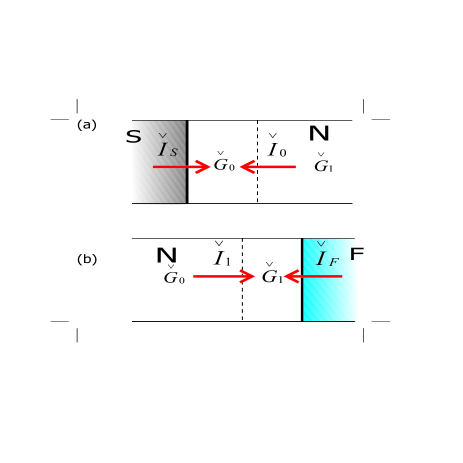
Figure 1: Matrix current and boundary conditions. Circuit-theory expressions give matrix currents $\hat{I}_{S},\hat{I}_{F}$ from the corresponding reservoirs. These currents should match matrix currents $\hat{I}_{0,1}$ from the Usadel equation, defined via derivatives of Green functions. This fixes the boundary conditions for the Usadel equation.

Circuit theory allows to find the boundary conditions at the interfaces of the normal metal in contact with the reservoirs simply by imposing matrix current conservation at these points. The matrix currents to the reservoirs are given by circuit theory expressions. (FIG. 1). We will assume that the superconducting reservoir is coupled to the normal metal through a tunnel contact. In addition, we disregard energy dependence of Green functions in the reservoir assuming that the energy scale of interest is much smaller than the superconducting energy gap $\Delta$ in the reservoir. Under these assumptions, the retarded Green function in the reservoir is just $\hat{\tau}_{1}$. The matrix current to the reservoir thus reads

$$\hat{I}_{S}=\frac{G_{S}}{2}\left[\hat{\tau}_{1},\hat{G}(x)\right].$$ (6)

To describe the matrix current to ferromagnetic insulator, we use the results of our previous work DaniCondmat where we obtain

$$\hat{I}_{F}=i\frac{G_{\phi}}{2}\left[\vec{M}\text{ }\hat{\vec{\sigma}}\text{ }\hat{\tau}_{3},\hat{G}(x)\right],$$ (7)

$\vec{\sigma}$ being matrices in spin space, $\vec{M}$ being the magnetization vector of the ferromagnet.

The parameter $G_{\phi}$ has a dimension of conductance and is related to the imaginary part of so-called mixing conductance $G_{\phi}=$Im$G^{\uparrow\downarrow}$. Mixing conductance has been introduced in Ref. Braatas, to describe the spin-flip of electrons reflected from a ferromagnetic boundary and is, in general, a complex number. For insulating ferromagnet it is however purely imaginary. In that case, $G_{\phi}$ acts as an effective magnetic field. Such spin-dependent scattering situation is shown to be important in magnetic insulator materials RefKumarPRL and half-metallic magnets. CuevasSDF Evaluation of $G_{\phi}$ for a simple model of insulating ferromagnet can be found in Ref. RefDaniPRLGBC, .

Using the parametrization in terms of $\theta(x)$, we find

$$\hat{I}_{S}=-G_{S}\cos\theta_{0}\text{ }\hat{\tau}_{2}\text{}$$ (8)

and

$$\hat{I}_{FI}=\pm iG_{\phi}\sin\theta_{1}\text{ }\hat{\tau}_{2}\text{,}$$ (9)

where the $+$($-$) sign corresponds to up (down) direction of spin with respect to the magnetization axis of the ferromagnet, $\theta_{0}=\theta(0)$ and $\theta_{1}=\theta(1)$.

Equating $\hat{I}_{S}=\hat{I}_{0},\hat{I}_{FI}=\hat{I}_{1}$ gives the boundary conditions required,

$$-g_{S}\cos\theta_{0}=\frac{\partial\theta(x)}{\partial x}|_{0}$$ (10)

$$\pm ig_{\phi}\sin\theta_{1}=\frac{\partial\theta(x)}{\partial x}|_{1}$$ (11)

where we have intoduced two important dimensionless parameters characterizing the stucture: $g_{S}=G_{S}/G_{N}$, $g_{\phi}=G_{\phi}/G_{N}$. As above, $\pm$ denotes two spin directions.

The solutions of the Usadel equation generally correspond to complex $\theta$. The density of states in a given point at a given energy is $\nu(\epsilon,x)=\nu_{0}\mbox{Re}[\cos(\theta(\epsilon,x))]$, $\nu_{0}$ being the density of states in the absence of proximity effect. In this paper, we concentrate on gap solutions where $\nu=0$ everywhere in the normal metal.

For this porpuse, it is convenient to define the complex angle $\theta(x)=\pi/2+i$ $\mu(x)$. Real $\mu(x)$ corresponds to gap solution. In terms of this angle, the full system to solve reads

$$\frac{\partial^{2}}{\partial x^{2}}\mu(x)+\tilde{\varepsilon}\cosh\mu(x)=0$$ (12)

$$+g_{S}\sinh\mu_{0}=\frac{\partial\mu(x)}{\partial x}|_{0}$$ (13)

$$\pm g_{\phi}\cosh\mu_{1}=\frac{\partial\mu(x)}{\partial x}|_{1}$$ (14)

where we introduce the dimensionless energy $\tilde{\varepsilon}=2$ $\varepsilon/E_{T}$. The gap solutions exist in a certain region of the three-dimensional parameter space $(g_{S},g_{\phi},\tilde{\varepsilon})$. To determine the boundary of this region is our primary task.

There are three limits where the solutions can be obtained analytically. The limit of vanishing resistance of the normal metal, $g_{S}\simeq g_{\phi}\simeq\tilde{\varepsilon}$, can be treated with cirquit theory and has been considered in Ref. RefDaniPRLGBC, . Below we address the zero energy limit ($\tilde{\varepsilon}\approx 0$) and ”spin-flip” limit ($g_{S}\simeq g^{2}_{\phi}\ll 1$).

IV Zero energy

Here we will analyze the gap solutions at the Fermi level, that is, at zero energy. In this case the leakage current conveniently dissapears, $\check{I}_{leakage}(x)=0$ and $\hat{I}$ = constant. Eq. (2) can be easily integrated giving $\hat{G}_{1}=\exp(\hat{I}/G_{N})\hat{G}_{0}$, where $\hat{G}_{0(1)}=\hat{G}(0(1))$. From this we obtain

$$\hat{I}=-\frac{G_{N}}{2}\frac{\arccos\left(\text{\mbox{Tr}}\left(\hat{G}_{{\bf 0}}\text{ }\hat{G}_{{\bf 1}}\right)\right)}{\sqrt{4-\left(\text{\mbox{Tr}}\left(\hat{G}_{{\bf 0}}\text{ }\hat{G}_{{\bf 1}}\right)\right)^{2}}}\left[\hat{G}_{{\bf 0}},\hat{G}_{{\bf 1}}\right],$$ (15)

which can be further simplified by using the parametrization $\hat{G}_{{\bf 0(1)}}=\cos\theta_{{\bf 0(1)}}$ $\hat{\tau}_{3}+\sin\theta_{{\bf 0(1)}}$ $\hat{\tau}_{1}$ into the following simple expression for the current through the diffusive normal metal:

$$\hat{I}=-i\ G_{N}(\theta_{0}-\theta_{1})\hat{\tau}_{2}=\ G_{N}(\mu_{0}-\mu_{1})\hat{\tau}_{2}.$$ (16)

Taking into account the boundary conditions on both interfaces, we obtain the equations for $\mu_{0,1}$,

$$g_{S}\sinh\mu_{0}=\mu_{1}-\mu_{0}=\pm g_{\phi}\cosh\mu_{1}.$$ (17)

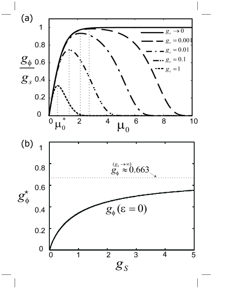
Figure 2: (a) $g_{\phi}/g_{S}$ versus $\mu_{0}$ for various values of $g_{S}$ (Eq.18). The maximum achieved at $\mu_{0}^{\ast}$ gives the maximum $g_{\phi}$ at which the gap persists at given $g_{S}$. (b) The maximum $g_{\phi}^{\ast}$ versus $g_{S}$. The curve saturates at $g_{\phi}\approx 0.663$ for $g_{S}\to\infty$.

We can readily express from these two equations $g_{\phi}/g_{S}$ as a function of $\mu_{0}$ and $g_{S}$

$$\frac{g_{\phi}}{g_{S}}=\frac{\sinh\mu_{0}}{\cosh\left(\mu_{0}+g_{S}\sinh\mu_{0}\right)}=f(\mu_{0},\text{ }g_{S})$$ (18)

Here we concentrate on the spin-up component. The solution for spin-down component corresponds to different sign of $\mu_{0}$. In FIG. 2a, we plot $g_{\phi}/g_{S}$ versus $\mu_{0}$ for several values of $g_{S}$. We see that $g_{\phi}/g_{S}$ reaches a maximum value $\left(g_{\phi}/g_{S}\right)^{\ast}$ at a certain value $\mu_{0}^{\ast}$. The position and the height of the maximum changes by changing $g_{S}$, $\mu(0)^{\ast}\to\infty,(g_{\phi}/g_{S})^{\ast}\to 1$ if $g_{S}\to 0$.

So for a given $g_{S}$, the maximum possible value of $g_{\phi}$ such as there is still a gap in the induced density of states of the wire is given by

$$g_{\phi}^{\ast}=f(\mu_{0}^{\ast},g_{S})g_{S}.$$ (19)

In FIG. 2b we plot $g_{\phi}^{\ast}$ as a function of $g_{S}$. This curve defines the boundary between gap (below) region and no gap (above) region in $g_{\phi}-g_{S}$ parameter space at zero energy $\varepsilon=0$. As expected, magnetic correlations combat the proximity effect at the Fermi level and the gap solutions dissapear upon increasing $g_{\phi}$. Even if the coupling to the superconductor is infinitely strong, $g_{S}\to\infty$, the gap survives only if $g_{\phi}<0.663$.

Let us expand $g_{\phi}/g_{S}$ near its maximum value $\left(g_{\phi}/g_{S}\right)^{\ast}$. Defining deviations from this point $\Delta g_{\phi-S}=\left(g_{\phi}/g_{S}\right)-\left(g_{\phi}/g_{S}\right)^{\ast}$ and $\bar{\mu}=\mu_{0}-\mu_{0}^{\ast}$, the expansion is obviously

$$\Delta g_{\phi-S}=-\text{ }C\text{ }\bar{\mu}^{2}$$ (20)

$C$ being a positive constant. Let us note that the density of states $\nu(0)/\nu_{0}=\mbox{Im}\ \sinh(\mu_{0})\propto\mbox{Im}\bar{\mu}$. This gives a square-root singularity of the density of states near the boundary,

$$\nu\propto\sqrt{\Delta g_{\phi-S}}.$$ (21)

The limit $g_{S}\rightarrow 0$ deserves some special consideration. It corresponds to the circuit-theory limit where the diffusive normal metal simply reduces to a “node” with spatially independent Green’s function $\check{G}$. This gives however, a BCS-like inverse square-root singularity in the density of states at the boundary given at $g_{S}=g_{\phi}$, $\nu/\nu_{0}=1/\sqrt{1-(g_{S}/g_{\phi})^{2}}\approx 1/\sqrt{2\Delta g_{\phi-S}}$ at $\Delta g_{\phi-S}\ll 1$. This result looks difficult to reconcile with the result obtained in Eq.(21).

The point is that for $g_{S}\ll 1$ an extra crossover takes place such the density of states changes from inverse square root to square root. The crossover occurs close to the gap boundary $g_{S}=g_{\phi}$. From Eq. (18) it is clear that for $g_{S}\ll 1$, the values of $g_{\phi}/g_{S}\simeq 1$ occur at $\mu_{0}\gg 1$. Close to the boundary, an expansion of Eq. (18) up to terms $\sim\exp({-2\mu_{0}})$ is possible. The evaluation of the maximum of $g_{\phi}/g_{S}$ as function of $\mu_{0}$ allows to determine the constant $C$ in Eq. (20), $C\simeq g_{S}^{4/3}$. The crossover occurs then at $\Delta g_{\phi-S}\simeq g_{S}^{2/3}\ll 1$. Below the crossover, at $\Delta g_{\phi-S}\ll g_{S}^{2/3}$, there is a square-root singularity $\nu/\nu_{0}\propto g^{-2/3}_{S}\sqrt{\Delta g_{\phi-S}}$ that changes to $\nu/\nu_{0}\simeq 1/\sqrt{2\Delta g_{\phi-S}}$ above the crossover, at $\Delta g_{\phi-S}\gg g_{S}^{2/3}$. The maximum density of states is therefore $\nu/\nu_{0}\simeq g_{S}^{-1/3}$.

V ”Spin-flip” limit

Now we would like to extend the results of the previous section to finite energy $\varepsilon$. We do this assuming that the Green function does not change much along the normal metal, so that $|\theta_{1}-\theta_{0}|\ll\theta_{0}$.

We start again with Eqs. (4), (10) and (11) . Integrating Eq.(4) over $x$ and using Eqs.(10) and (11) gives

$$\pm ig_{\phi}\sin\theta_{1}+g_{S}\cos\theta_{0}+i\text{ }\tilde{\varepsilon}\int_{0}^{1}dx\sin\theta(x)=0.$$ (22)

If we assume that the Green function does not change with $x$, $\theta(x)=\theta_{0}$, we derive from Eq. (22) the circuit-theory equation

$$i\left(\tilde{\varepsilon}\text{ }\pm g_{\phi}\right)\sin\theta_{0}+g_{S}\cos\theta_{0}=0.$$ (23)

With this, we reproduce the results dicussed in Ref.RefDaniPRLGBC, : the density of states mimics the one of a BCS superconductor in the presence of the spin-splitting magnetic field

$$\upsilon(\tilde{\varepsilon})=\frac{\left|\tilde{\varepsilon}\pm g_{\phi}\right|}{\sqrt{(\tilde{\varepsilon}\pm g_{\phi})^{2}-g_{S}^{2}}}.$$ (24)

The presence of a gap is strictly speaking a non-perturbative effect. The perturbation expansion of the density of states shown in Eq. (24) is valid at high energies $|\varepsilon\pm\tilde{h}|\gg\tilde{\Delta}$. The leading “spin-dependent” correction is proportional to $(\tilde{\Delta}^{2}\tilde{h})/\varepsilon^{3}\equiv(g_{S}^{2}g_{\phi})/\tilde{\varepsilon}^{3}$. This implies that the leading diagram in perturbation series involves four tunneling amplitudes at the $S/N$ interface and two spin-dependent reflection amplitudes at the $N/FI$ interface.

The equation (23) is correct in the leading order in $\tilde{\varepsilon},g_{S},g_{\phi}\ll 1$. There can be however a problem if $\tilde{\varepsilon}$ is too close to $\mp g_{\phi}$ since the first coefficient is anomalously small in this case. To account for this, we should re-derive these equations to the next-to-leading order.

We present $\theta(x)$ in the form that satisfies boundary conditions,

$$\theta(x)=\theta_{0}+\left(\theta_{1}-\theta_{0}\right)x+\theta^{(1)}(x);\;\theta^{(1)}(0)=\theta^{(1)}(1)=0$$ (25)

and evalutate the corrections $\theta_{1}-\theta_{0},\theta^{(1)}(x)$ in the leading order. To evaluate $\theta_{1}-\theta_{0}$, let us multiply Eq.(4) by $x$ and integrate by parts the first term $\int_{0}^{1}dx$ $x$ $\ddot{\theta}(x)$ where ($\ddot{\theta}(x)\equiv\partial^{2}\theta(x)/\partial x^{2}$), obtaining the following expression

$$\dot{\theta}_{1}-\left(\theta_{1}-\theta_{0}\right)+i\text{ }\tilde{\varepsilon}\int_{0}^{1}dx\text{ }x\text{ }\sin\theta(x)=0.$$ (26)

We set $\theta(x)=\theta_{0}$ under the sign of integral and use Eq. (11) to obtain

$$\theta_{1}-\theta_{0}=i\left(\pm g_{\phi}\text{ }+\frac{\tilde{\varepsilon}}{2}\right)\sin\theta_{0}.$$ (27)

With the same accuracy, the differential equation for $\theta^{(1)}(x)$ reads

$$\frac{\partial^{2}}{\partial x^{2}}\theta^{(1)}(x)+i\text{ }\tilde{\varepsilon}\sin\left(\theta_{0}\right)=0.$$ (28)

This results in

$$\theta^{(1)}(x)\approx i\text{ }\tilde{\varepsilon}\frac{\sin\theta_{0}}{2}(x-x^{2}).$$ (29)

Finally we substitute Eqs. (29) to Eq. (22) to get the following relation:

$$i\left(\tilde{\varepsilon}\text{ }\pm g_{\phi}\right)\sin\theta_{0}+g_{S}\cos\theta_{0}-\zeta g_{S}\sin\theta_{0}\cos\theta_{0}=0,$$ (30)

where $\zeta=\left(g_{\phi}^{2}\pm g_{\phi}\tilde{\varepsilon}+\tilde{\varepsilon}^{2}/3\right)/g_{S}$. As we mentioned above, $\zeta$ plays a role only if $|\tilde{\varepsilon}\text{ }\pm g_{\phi}|\ll\tilde{\varepsilon},g_{\phi}$. Under these conditions, the energy dependence of $\zeta$ can be disregarded and $\zeta=g_{\phi}^{2}/3g_{S}$.

The relation (30) resembles very much one of the most important equations in the superconductivity theory that was first derived by Abrikosov and Gor’kov AG to describe suppresion of superconductivity by magnetic impurities. Precise association is achieved by the following change of notations:

$$(\tilde{\varepsilon}\pm g_{\phi})E_{T} \to E,$$

$$g_{S}E_{T} \to \Delta,$$

$$\zeta\Delta=E_{T}g^{2}_{\phi}/3 \to 1/\tau_{s}$$

where $E,\Delta,\tau_{s}$ are respectively energy, superconducting order parameter and spin-flip time due to magnetic impurities.AG This is why we refer to the limit under consideration as to ”spin-flip” limit. To remind, there are no magnetic impurities in the structure considered, and effective spin-flip comes from interplay of diffusion in the normal metal and reflection at the $N/FI$ interface.

Maki has demonstrated that similar equation accounts for gapless superconductivity in a variety of circumstances, $\zeta$ being the pair-breaking parameter.MakiFDS We define $\theta_{0}=\pi/2+i$ $\mu_{0}$, $u=\tanh\mu_{0}$, $\omega=\left(\tilde{\varepsilon}\text{ }\pm g_{\phi}\right)/g_{S}$, to be close to notations of Ref. MakiFDS, . This gives

$$\omega=u\left(1-\zeta\frac{1}{\sqrt{1-u^{2}}}\right)$$ (31)

The maximum value of $\omega$ with respect to real $u$, $\omega^{\ast}$ gives the energy interval around $\tilde{\varepsilon}=\mp g_{\phi}$ where the gap solutions occur. This value is determined by the condition $\partial\omega/\partial u=0$, which gives

$$\omega^{\ast}=\text{ }\left(1-\zeta^{2/3}\right)^{3/2}$$ (32)

achieved at $u=u^{*}$,

$$u^{\ast}=\left(1-\zeta^{2/3}\right)^{1/2}.$$ (33)

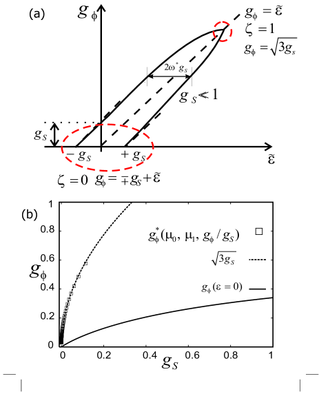
Figure 3: (a) The sketch of the gap domain in $\tilde{\varepsilon}-g_{\phi}$ plane at $g_{S}\ll 1$. (b) Exact results (squares) for the maximum $g_{\phi}$ at $\zeta=1$, follow the expected $\sqrt{3g_{S}}$ dependence for small $g_{S}$. The lower curve is the one plotted in FIG. 2.

There are no gap solutions if $\zeta>1$. The region where these solutions do occur is sketched in FIG. 3a in $\tilde{\varepsilon}-g_{\phi}$ coordinates. It looks like a $45^{\circ}$ slanted strip, the width of the stip in horizontal direction being given by $2\omega^{\ast}g_{S}$. Near the origin $\zeta=0$. In this situation, it is obtained from Eqs.(32, 33) that the width is $2g_{S}$ and $|\tilde{\varepsilon}\pm g_{\phi}|=g_{S}$. The gap solutions at zero energy $\tilde{\varepsilon}=0$ dissapear at $g_{\phi}=g_{S}$. The width gradualy reduces with increasing $g_{\phi}$ due to the increase of $\zeta$. The strip ends if $\zeta=1$, that is, at $|g_{\phi}|=\sqrt{3g_{S}}\gg g_{S}$ (FIG. 3b).

This demonstrates that even in the limit of $g_{\phi},g_{S}\ll 1$ the ferromagentic insulator not only shifts the gap states but also reduces and finally suppesses the gap due to effective spin-flip. We show in the next section that the same picture is qualitatively valid for arbitrary values of these parameters.

VI gap-no gap boundary in general case

So far we have studied the boundary separating gap and no-gap solutions in the parameter space for two limiting cases that allow for analytic solutions. In this section, we find this boundary for arbitrary values of the parameters. We do this by solving Eqs. (12,13,14) numerically.

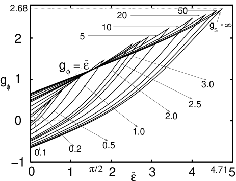
Figure 4: The gap domains (strips) in $g_{\phi}-\tilde{\varepsilon}$ plane calculated for different values of $g_{S}=[0.1,0.2,..,50,\infty]$. Their shape is similar to the sketch in FIG. 3a. The tip of each strip gives the maximum value of $g_{\phi}$ at which the gap survives and simultaneously the corresponding energy.

Figure 5: Side view of the boundary surface in three-dimensional ($g_{S},g_{\phi},\tilde{\varepsilon}$) space. The upper curve gives the maximum $g_{\phi}$ connecting the tips of the strips plotted in FIG.4. It rises monotonically with $g_{S}$ to reach the asymptotic value $\simeq 2.68$ at $g_{S}\rightarrow\infty$. The lower curve presents a cross-section of the surface with the $\tilde{\varepsilon}=0$ plane.

Since we only concern with the boundary, the numerical procedure is as follows. We fix $g_{S}$ and $\tilde{\varepsilon}$. The solutions of Eq. 12 with boundary condition (13) can be parametrized with $\mu_{0}$. We express $\mu_{1},\dot{\mu}_{1}$ in terms of $\mu_{0}$. Then the last boundary condition (14) could be solved to find $\mu_{0}$ in terms of $g_{\phi}$. We do the opposite: We use (14) to directly express $g_{\phi}$ in terms of $\mu_{0}$ and find the two extrema of $g_{\phi}(\mu_{0})$. Those give the endpoints of the interval of $g_{\phi}$ where the gap solutions exist — elements of the boundary. We plot these endpoins at fixed $g_{S}$ versus dimensionless energy $\tilde{\varepsilon}$ to obtain slanted strips similar to the one in FIG. 3a. At certain energy, the extrema come together indicating the endpoint of the strip.

In FIG. 4 we show these strips in $g_{\phi}-\tilde{\varepsilon}$ plane for a wide range of values of $g_{S}$. As expected from the previous discussion, for $g_{S}\ll 1$ the strips extend along the $g_{\phi}=\tilde{\varepsilon}$ line. The sharp tip of each strip gives the critical value of $g_{\phi}$ at which for a given $g_{S}$ the induced minigap disappears. For small $g_{S}$, the height of the tip, $\sqrt{3g_{S}}$, is much bigger than the width of the strip $g_{S}$. With increasing $g_{S}$, the shape of the strips changes. They increase both in width and height, so that these dimensions become of the same order. The strips also become less slanted. The shape converges at $g_{S}\to\infty$ (outer curve in FIG.4). In this limit, the maximum $g_{\phi}$ that allows for superconductivity is $\approx 2.68$ and is achieved at $\tilde{\varepsilon}\approx 4.71$. It is interesting to note that this energy is higher than the maximum value of the minigap without magnetic correlations ($\tilde{\varepsilon}(g_{\phi}=0)=\pi/2,$ see FIG. 4). Counterintuitevely, the presence of the magnetic insulator helps the gap solutions to persist at higher energy. Albeit the magnetic correlations quickly remove these solutions from the Fermi level.

Each strip is a cross-section of the boundary surface in three-dimensional $(g_{\phi},g_{S},\tilde{\varepsilon})$ space. We present in FIG. 5 the side view of this surface. The lower curve in this figure is the cross-section of the surface with $\tilde{\varepsilon}=0$ plane and shows the critical value of $g_{\phi}$ at which the gap solutions dissapear from the Fermi level. The same curve has been already presented in FIG. 2. The upper curve gives the critical value of $g_{\phi}$ at which gap solutions dissapear at any energy. It consists of the tips of each strip from FIG. 4 as a function of $g_{S}$. We see that at $g_{S}\to\infty$ this curve satures at $g_{\phi}=2.68$. The asymptotics $g_{\phi}=\sqrt{3g_{S}}$ derived in the previous section agree with this curve at $g_{\phi}<1$ as expected.

VII Conclusions

We have studied the proximity effect in $S/N/FI$ structures with N being a diffusive normal metal. We pay special attention to the gap in the density of states and find its domain in the parameter space. The convenient dimensionless parameters to work with are $g_{\phi},g_{S}$ that characterize the intensity of magnetic and superconducting correlations respectively, and energy in units of Thouless energy, $\tilde{\varepsilon}$.

We demonstrate that the combined effect of a ferromagnetic insulator and the elastic scattering on the proximity gap of a diffusive wire is twofold. First, the ferromagnetic insulator provides an effective exchange field $\tilde{h}$ that shifts the gap edges in opposite directions for opposite components without reducing the energy interval where the gap solutions occur. Second, its effect combined with suficiently strong elastic scattering in N reduces this interval and finally suppresses the gap. In the limit of small $g_{S},g_{\phi}$ (”spin-flip” limit) the mechanism of this suppression is precisely equivalent to the known one from magnetic impurities, with an effective spin-flip rate $1/\tau_{s}=g_{\phi}^{2}E_{T}/3$. Qualitatively, this picture remains valid at arbitrary parameters.

If $g_{\phi}>0.66$ no gap persist at the Fermi level. If $g_{\phi}>2.68$ no gap occurs at any energy. Counterintuitively, the gap in the presence of magnetic correlations may occur at energies higher than in the absence of the ferromagnetic insulator.

The absence or the presence of the gap in the normal part of a $S/N/FI$ structure at certain energy can be observed by a spin-sensitive tunnel probe. The resistance of such probe must exceed all interface resistances. The possible implementation of the probe depends on its concrete geometry. For traditional sandwich geometry, it is probably simpler to keep the $FI$ layer rather thin, so that the electrons can tunnel through. Covering this layer with a conducting ferromagnet makes the tunnel probe. For the wire geometry, small tunnel contacts to ferromagnets can be made in different points of the normal wire. An alternative is the suggestion of Ref. RefDaniPRLGBC, : the tunneling between two $FI/N/S$ structures.

We thank W. Belzig, D. Esteve and Ya. M. Blanter for useful discussions. This work was financially supported by the Stichting voor Fundamenteel Onderzoek der Materie (FOM). D. H-H also acknowledges additional financial support from the U.S. DOE grant DE-FG-0291-ER-40608.

References

- (1) G. Deutscher and P.G. de Gennes, in Superconductivity, edited by R.D. Parks (Dekker, New York, 1969), p. 1005;P.G. de Gennes, Phys. Lett. 23, 10 (1969); G. Deutscher and F. Meunier, Phys. Rev. Lett. 22,395 (1969); J. J. Hauser Phys. Rev. Lett. 23,374 (1969);
- (2) V.V. Ryazanov, V.A. Oboznov, A.Y. Rusanov, A.V. Veretennikov, A.A. Golubov, and J. Aarts, Phys. Rev. Lett. 86, 2427 (2001); T. Kontos, M. Aprili, J. Lesueur, F. Genet, B. Stephanidis, and R.Boursier, Phys. Rev. Lett. 89, 137007 (2002).
- (3) A.I. Buzdin, A.V. Vedyayev, and N.V. Ryzhanova, Europhys. Lett. 48, 686 (1999); L. R. Tagirov, Phys. Rev. Lett. 83, 2058 (1999).
- (4) A. F. Volkov, F. S. Bergeret and K. B. Efetov, Phys. Rev. Lett. 90, 117006 (2003); F. S. Bergeret, A. F. Volkov, and K. B. Efetov, Phys. Rev. Lett. 86, 4096 (2001).
- (5) R. Mélin and S. Peysson, Phys. Rev. B 68, 174515 (2003); R. Mélin, Eur. Phys. J B 39, 249 (2004); R. Mélin and D. Feinberg, cond-mat/0407283.
- (6) G. Falci, D. Feinberg, and F. W. J. Hekking, Europhys. Lett. 54, 225 (2001); N. M. Chtchelkatchev, JETP Lett. 78, 230 (2003).
- (7) P.M. Tedrow and R. Meservey, Phys. Rev. Lett. 27, 919 (1971); R. Meservey and P.M. Tedrow, Phys. Rep. 238, 173 (1994); J. Y. Gu, C.-Y. You, J. S. Jiang, J. Pearson, Ya. B. Bazaliy, and S. D. Bader, Phys. Rev. Lett. 89,267001 (2002).
- (8) R. Fazio and C. Lucheroni, Europhys. Lett. 45, 707 (1999); K. Halterman and O. T. Valls, Phys. Rev. B 65, 014509 (2001); ibid. B 66, 224516 (2002); B 69, 014517 (2004); F. S. Bergeret, A. F. Volkov and K. B. Efetov, Phys. Rev. B 65, 134505 (2002).
- (9) A. A. Abrikosov, L. P. Gorkov Sov. Phys. JETP-USSR 12, 1243 (1961).
- (10) M.J. DeWeert and G.B. Arnold, Phys. Rev. Lett. 55, 1522 (1985); M.J. DeWeert and G.B. Arnold, Phys. Rev. B 39, 11307 (1989).
- (11) T. Tokuyasu, J.A. Sauls and D. Rainer, Phys. Rev. B 38, 8823 (1988).
- (12) P. M. Tedrow, J. E. Tkaczyk and A. Kumar, Phys. Rev. Lett. 56, 1746 (1986).
- (13) D. Huertas-Hernando, Yu. V. Nazarov and W. Belzig, Phys. Rev. Lett. 88,047003 (2002).
- (14) A. F. Andreev, Sov. Phys. JETP 19,1228 (1964).
- (15) M. Tinkham, Introduction to Superconductivity, 2nd ed., (McGraw Hill, N.Y., 1996).
- (16) I. O. Kulik, Sov. Phys. JETP 30, 944 (1970).
- (17) W.L. McMillan, Phys. Rev. 175, 537 (1968).
- (18) S. Guéron, H. Pothier, Norman O. Birge, D. Esteve, and M. H. Devoret , Phys. Rev. Lett. 77, 3025(1996); W. Belzig, C. Bruder and G. Schön, Phys. Rev. B 54, 9443 (1996); E. Scheer, W. Belzig, Y. Naveh, M. H. Devoret, D. Esteve, and C. Urbina , Phys. Rev. Lett. 86, 284 (2001); N. Moussy, H. Courtois and B. Pannetier, Europhys. Lett.55, 861 (2001).
- (19) A. A. Golubov and M. Yu. Kupriyanov, Sov Phys. JETP 69, 805 (1989); A. Lodder and Yu. V. Nazarov, Phys. Rev. B 58, 5783 (1998); S. Pilgram, W. Belzig and C. Bruder, Phys. Rev. B 62, 12462 (2000); P. M. Ostrovsky, M. A. Skvortsov and M. V. Feigel’man, Phys. Rev. Lett. 87, 027002 (2001).
- (20) K. D. Usadel, Phys. Rev. Lett. 25, 507 (1970).
- (21) A.V. Zaitsev, Sov. Phys. JETP 59, 1015 (1984).
- (22) A. Millis, D. Rainer and J.A. Sauls, Phys. Rev. B 38, 4504 (1988).
- (23) Yu. V. Nazarov, Phys. Rev. Lett. 73, 1420 (1994); Yu.V. Nazarov, Superlatt. and Microstruc. 25, 1221 (1999).
- (24) J. Kopu, M. Eschrig, J.C. Cuevas, and M. Fogelstrom, Phys. Rev. B 69, 094501 (2004).
- (25) M. Zareyan, W. Belzig and Yu. V. Nazarov, Phys. Rev. Lett. 86, 308 (2001).
- (26) J. Rammer and H. Smith, Rev. Mod. Phys. 58, 323 (1986).
- (27) D. Huertas-Hernando, W. Belzig and Yu. V. Nazarov, cond-mat/0204116.
- (28) A. Brataas, Yu. V. Nazarov and G.E.W. Bauer, Phys. Rev. Lett. 84, 2481 (2000).
- (29) M. Eschrig, J. Kopu, J. C. Cuevas and G. Schön, Phys. Rev. Lett. 90, 137003 (2003).
- (30) K. Maki Gapless Superconductivity, chap. 18, Vol. 2 in Superconductivity, edited by R.D. Parks (Marcel Dekker, New York, 1969).