Periodic Anderson model with degenerate orbitals:
linearized dynamical mean field theory approach

1 Introduction

Since the discovery of heavy-fermion materials with rare-earth or actinide elements, comprehensive understanding of this class of correlated electron systems has received considerable attention. In these compounds, strong correlations among $f$ electrons play an important role to form the heavy quasi-particle state at low temperatures. In particular, if correlated $f$-electron systems are in the insulating phase, they are referred to as the Kondo insulator, which possesses a wide variety of compounds. ${}^{\hbox{\immediate{\bf{?}},\penalty 1000\hskip 0.91003pt plus 0.70004pt minus 0.70004pt{\bf{?}},\penalty 1000\hskip 0.91003pt plus 0.70004pt minus 0.70004pt{\bf{?}},\penalty 1000\hskip 0.91003pt plus 0.70004pt minus 0.70004pt{\bf{?}},\penalty 1000\hskip 0.91003pt plus 0.70004pt minus 0.70004pt{\bf{?}},\penalty 1000\hskip 0.91003pt plus 0.70004pt minus 0.70004pt{\bf{?}},\penalty 1000\hskip 0.91003pt plus 0.70004pt minus 0.70004pt{\bf{?}},\penalty 1000\hskip 0.91003pt plus 0.70004pt minus 0.70004pt{\bf{?}},\penalty 1000\hskip 0.91003pt plus 0.70004pt minus 0.70004pt{\bf{?}},\penalty 1000\hskip 0.91003pt plus 0.70004pt minus 0.70004pt{\bf{?}})}}$ To discuss the electronic properties theoretically, the periodic Anderson model (PAM) has been investigated extensively. This model is simplified to extract the essence of heavy fermions, which is usually described by free conduction electrons coupled to highly correlated single-orbital $f$ electrons.

In some heavy-fermion compounds, the other parameters dropped in the original PAM, such as the orbital degeneracy and the interactions among conduction electrons, are also important to explain the experimental findings. For example, the compound Nd_2-xCe_xCuO₄ ${}^{\hbox{\immediate{\bf{?}},\penalty 1000\hskip 0.91003pt plus 0.70004pt minus 0.70004pt{\bf{?}},\penalty 1000\hskip 0.91003pt plus 0.70004pt minus 0.70004pt{\bf{?}},\penalty 1000\hskip 0.91003pt plus 0.70004pt minus 0.70004pt{\bf{?}},\penalty 1000\hskip 0.91003pt plus 0.70004pt minus 0.70004pt{\bf{?}})}}$ shows the unusual behavior in the specific heat, which may be explained by properly taking into account the correlations due to not only $f$ electrons but also conduction electrons. Furthermore, it is claimed that the orbital degrees of freedom affect the Kondo-insulating gap around Fermi surface for another prototype of heavy fermion compound, $\rm YbBe_{12}$.${}^{\hbox{\immediate{?},\penalty 1000\hskip 0.91003pt plus 0.70004pt minus 0.70004pt{?},\penalty 1000\hskip 0.91003pt plus 0.70004pt minus 0.70004pt{?})}}$ These findings naturally encourage us to explore the effects beyond the simple PAM systematically, such as correlations due to conduction electrons, the orbital effects, etc.

In this paper, we investigate the doubly degenerate periodic Anderson model to discuss the effects on the Kondo insulator due to orbital degeneracy together with electron correlations for $f$ and conduction bands. By exploiting a linearized version of dynamical mean field theory (DMFT), we show that the interplay of several interactions yields interesting effects on the formation of the Kondo insulator, which do not appear in the simple PAM.

This paper is organized as follows. In §2, we introduce the model Hamiltonian with orbital degeneracy, and then briefly explain a linearized version of DMFT. In §3, we discuss electron correlations due to conduction bands by employing the single-orbital model. We then explore in §4 how the interplay of several distinct interactions in the degenerate model produces nontrivial effects on the low-energy electronic properties. A brief summary is given in the last section.

2 Model Hamiltonian and Method

2.1 Two-orbital periodic Anderson model

We consider the periodic Anderson model with two-fold degenerate orbitals, which may be described by the following Hamiltonian,

$${\cal H}_{PAM} = {\cal H}_{0}+{\cal H}_{I}$$ (1)

$${\cal H}_{0} = \sum_{\stackrel{{\scriptstyle<i,j>}}{{m,\sigma}}}t_{ij}c^{{\dagger}}_{im\sigma}c_{jm\sigma}+\sum_{i,m,\sigma}\epsilon_{f}f^{{\dagger}}_{im\sigma}f_{im\sigma}$$ (2)

$$+ V\sum_{i,m,\sigma}\left(f^{{\dagger}}_{im\sigma}c_{im\sigma}+h.c.\right)$$

$${\cal H}_{I} = U_{f}\sum_{i,m}n^{f}_{im\uparrow}n^{f}_{im\downarrow}+U_{c}\sum_{i,m}n^{c}_{im\uparrow}n^{c}_{im\downarrow}$$ (3)

$$+ U^{\prime}_{f}\sum_{i,\alpha,\beta}n^{f}_{i1\alpha}n^{f}_{i2\beta}+U^{\prime}_{c}\sum_{i,\alpha,\beta}n^{c}_{i1\alpha}n^{c}_{i2\beta}$$

$$- J_{f}\sum_{i}{\bf S}^{f}_{i1}\cdot{\bf S}^{f}_{i2}-J_{c}\sum_{i}{\bf S}^{c}_{i1}\cdot{\bf S}^{c}_{i2}$$

where $f_{im\sigma}(c_{im\sigma})$ annihilates an $f$ electron (conduction electron) with spin $\sigma(=\uparrow,\downarrow)$ and orbital $m(=1,2)$ at the $i$th site, $n_{im\sigma}^{c}=c_{im\sigma}^{\dagger}c_{im\sigma}$ and $n_{im\sigma}^{f}=f_{im\sigma}^{\dagger}f_{im\sigma}$. Here, $t_{ij}$ represents the hopping integral, $\epsilon_{f}$ the energy level of the $f$ state, and $V$ the hybridization between the conduction and $f$ states. $U_{f}(U_{c})$ is the intra-orbital Coulomb interaction, $U^{\prime}_{f}(U^{\prime}_{c})$ is the inter-orbital Coulomb interaction, and $J_{f}(J_{c})$ is Hund coupling for $f$ electrons (conduction electrons). The spin operators are defined by ${\bf S}_{im}^{f}=\frac{1}{2}\sum_{\alpha\beta}f^{{\dagger}}_{im\alpha}{\bf\tau}_{\alpha\beta}f_{im\beta}$ and ${\bf S}_{im}^{c}=\frac{1}{2}\sum_{\alpha\beta}c^{{\dagger}}_{im\alpha}{\bf\tau}_{\alpha\beta}c_{im\beta}$, where ${\bf\tau}$ is the Pauli matrix. Note that the model has two orbitals both for conduction and $f$ electrons, which are specified by the same index, $m$. This scheme has been sometimes used for investigating the orbital effects on heavy fermion systems, which may capture some essential properties due to degenerate orbitals. ${}^{\hbox{\immediate{\bf{?}},\penalty 1000\hskip 0.91003pt plus 0.70004pt minus 0.70004pt{\bf{?}},\penalty 1000\hskip 0.91003pt plus 0.70004pt minus 0.70004pt{\bf{?}})}}$ In this paper, we discuss how electron correlations are developed in the Kondo insulator with multi-orbitals, by changing the parameters $\{U_{f},U_{f}^{\prime},J_{f}\}$ and $\{U_{c},U_{c}^{\prime},J_{c}\}$ systematically.

2.2 Linearized dynamical mean-field theory

We make use of DMFT, which has been developed by several groups${}^{\hbox{\immediate{\bf{?}},\penalty 1000\hskip 0.91003pt plus 0.70004pt minus 0.70004pt{\bf{?}},\penalty 1000\hskip 0.91003pt plus 0.70004pt minus 0.70004pt{\bf{?}},\penalty 1000\hskip 0.91003pt plus 0.70004pt minus 0.70004pt{\bf{?}})}}$ and has successfully been applied to the single-band Hubbard model, ${}^{\hbox{\immediate{?},\penalty 1000\hskip 0.91003pt plus 0.70004pt minus 0.70004pt{\bf{?}},\penalty 1000\hskip 0.91003pt plus 0.70004pt minus 0.70004pt{\bf{?}},\penalty 1000\hskip 0.91003pt plus 0.70004pt minus 0.70004pt{\bf{?}},\penalty 1000\hskip 0.91003pt plus 0.70004pt minus 0.70004pt{\bf{?}},\penalty 1000\hskip 0.91003pt plus 0.70004pt minus 0.70004pt{\bf{?}},\penalty 1000\hskip 0.91003pt plus 0.70004pt minus 0.70004pt{\bf{?}},\penalty 1000\hskip 0.91003pt plus 0.70004pt minus 0.70004pt{\bf{?}},\penalty 1000\hskip 0.91003pt plus 0.70004pt minus 0.70004pt{\bf{?}},\penalty 1000\hskip 0.91003pt plus 0.70004pt minus 0.70004pt{\bf{?}},\penalty 1000\hskip 0.91003pt plus 0.70004pt minus 0.70004pt{\bf{?}})}}$ the two-band Hubbard model, ${}^{\hbox{\immediate{?},\penalty 1000\hskip 0.91003pt plus 0.70004pt minus 0.70004pt{\bf{?}},\penalty 1000\hskip 0.91003pt plus 0.70004pt minus 0.70004pt{\bf{?}},\penalty 1000\hskip 0.91003pt plus 0.70004pt minus 0.70004pt{\bf{?}},\penalty 1000\hskip 0.91003pt plus 0.70004pt minus 0.70004pt{\bf{?}},\penalty 1000\hskip 0.91003pt plus 0.70004pt minus 0.70004pt{\bf{?}},\penalty 1000\hskip 0.91003pt plus 0.70004pt minus 0.70004pt{\bf{?}},\penalty 1000\hskip 0.91003pt plus 0.70004pt minus 0.70004pt{\bf{?}},\penalty 1000\hskip 0.91003pt plus 0.70004pt minus 0.70004pt{\bf{?}},\penalty 1000\hskip 0.91003pt plus 0.70004pt minus 0.70004pt{\bf{?}},\penalty 1000\hskip 0.91003pt plus 0.70004pt minus 0.70004pt{\bf{?}},\penalty 1000\hskip 0.91003pt plus 0.70004pt minus 0.70004pt{\bf{?}},\penalty 1000\hskip 0.91003pt plus 0.70004pt minus 0.70004pt{\bf{?}},\penalty 1000\hskip 0.91003pt plus 0.70004pt minus 0.70004pt{\bf{?}})}}$ the PAM ${}^{\hbox{\immediate{\bf{?}},\penalty 1000\hskip 0.91003pt plus 0.70004pt minus 0.70004pt{\bf{?}},\penalty 1000\hskip 0.91003pt plus 0.70004pt minus 0.70004pt{\bf{?}},\penalty 1000\hskip 0.91003pt plus 0.70004pt minus 0.70004pt{\bf{?}},\penalty 1000\hskip 0.91003pt plus 0.70004pt minus 0.70004pt{\bf{?}},\penalty 1000\hskip 0.91003pt plus 0.70004pt minus 0.70004pt{?})}}$ , etc. This treatment can take into account local electron correlations precisely, and thereby is exact in infinite dimensions. Then the lattice model can be mapped onto an effective impurity model, which has been solved by a variety of methods such as the iterated perturbation theory, ${}^{\hbox{\immediate{?},\penalty 1000\hskip 0.91003pt plus 0.70004pt minus 0.70004pt{?},\penalty 1000\hskip 0.91003pt plus 0.70004pt minus 0.70004pt{?})}}$ the non-crossing approximation, ${}^{\hbox{\immediate{\bf{?}},\penalty 1000\hskip 0.91003pt plus 0.70004pt minus 0.70004pt{?},\penalty 1000\hskip 0.91003pt plus 0.70004pt minus 0.70004pt{?})}}$ the projective self-consistent method. ${}^{\hbox{\immediate{?},\penalty 1000\hskip 0.91003pt plus 0.70004pt minus 0.70004pt{?})}}$ Since these methods are not efficient enough to treat the systems with degenerate orbitals, powerful numerical methods have been employed, e.g. the exact diagonalization, ${}^{\hbox{\immediate{?},\penalty 1000\hskip 0.91003pt plus 0.70004pt minus 0.70004pt{?},\penalty 1000\hskip 0.91003pt plus 0.70004pt minus 0.70004pt{?},\penalty 1000\hskip 0.91003pt plus 0.70004pt minus 0.70004pt{?})}}$ the quantum Monte Carlo simulation. ${}^{\hbox{\immediate{?},\penalty 1000\hskip 0.91003pt plus 0.70004pt minus 0.70004pt{?},\penalty 1000\hskip 0.91003pt plus 0.70004pt minus 0.70004pt{?},\penalty 1000\hskip 0.91003pt plus 0.70004pt minus 0.70004pt{?},\penalty 1000\hskip 0.91003pt plus 0.70004pt minus 0.70004pt{?},\penalty 1000\hskip 0.91003pt plus 0.70004pt minus 0.70004pt{?})}}$ Recently a new method to solve the effective impurity model has been proposed by Potthoff,${}^{\hbox{\immediate{?})}}$ which we will refer to the linearized DMFT in this paper. This approach simplifies the procedure of DMFT by linearizing the self-consistent equations in the low-energy region, but still keeps the essential features of electron correlations. In this approximation, the effective bath is represented by a few sites. In spite of this simplification, electronic properties in the low-energy region around the Fermi surface can be described rather well.${}^{\hbox{\immediate{?},\penalty 1000\hskip 0.91003pt plus 0.70004pt minus 0.70004pt{?})}}$ In fact, the critical values of the Hubbard model with and without degenerate orbitals are in good agreement with the other numerical techniques.${}^{\hbox{\immediate{?},\penalty 1000\hskip 0.91003pt plus 0.70004pt minus 0.70004pt{?})}}$

In this paper, we exploit the linearized DMFT, which may convert the original model eq. (1) to the effective impurity Anderson model,

$${\cal H}_{imp} = \sum_{lm\sigma}\tilde{\varepsilon}_{l}d^{{\dagger}}_{lm\sigma}d_{lm\sigma}+\sum_{lm\sigma}\tilde{V}_{l}\left(d^{{\dagger}}_{lm\sigma}c_{m\sigma}+h.c.\right)$$ (4)

$$+ \tilde{\varepsilon}_{c}\sum_{lm\sigma}c^{{\dagger}}_{m\sigma}c_{m\sigma}+\tilde{\varepsilon}_{f}\sum_{lm\sigma}f^{{\dagger}}_{m\sigma}f_{m\sigma}$$

$$+ V\sum_{lm\sigma}\left(f^{{\dagger}}_{m\sigma}c_{m\sigma}+h.c.\right)$$

$$+ U_{f}\sum^{2}_{m=1}n^{f}_{m\uparrow}n^{f}_{m\downarrow}+U_{c}\sum^{2}_{m=1}n^{c}_{m\uparrow}n^{c}_{m\downarrow}$$

$$+ U^{\prime}_{f}\sum_{\alpha,\beta}n^{f}_{1\alpha}n^{f}_{2\beta}+U^{\prime}_{c}\sum_{\alpha,\beta}n^{c}_{1\alpha}n^{c}_{2\beta}$$

$$- J_{f}{\bf S}^{f}_{1}\cdot{\bf S}^{f}_{2}-J_{c}{\bf S}^{c}_{1}\cdot{\bf S}^{c}_{2}$$

where $\tilde{\epsilon}_{c}$ and $\tilde{\epsilon}_{f}$ are the renormalized energy levels, which should be determined by the number of conduction and $f$ electrons in the system. Here, $d^{{\dagger}}_{lm\sigma}(d_{lm\sigma})$ creates (annihilates) an electron in the effective bath with two sites $(l=1,2)$.

To determine the effective energy $\tilde{\varepsilon}_{l}$ and the hybridization $\tilde{V}_{l}$, we linearize the self-energies in the small $\omega$ region as,

$$\begin{array}[]{rcl}\Sigma^{ff}(\omega)&=&a+b\omega+O(\omega^{2})\\ \Sigma^{cc}(\omega)&=&c+d\omega+O(\omega^{2})\\ \Sigma^{fc}(\omega)&=&g+h\omega+O(\omega^{2}),\end{array}$$ (5)

where $a,b,c,d,g$ and $h$ are real numbers to be determined. The renormalization factors for $f$ and conduction electrons are respectively given as,

$$Z_{f} = (1-b)^{-1}$$ (6)

$$Z_{c} = (1-d)^{-1}.$$ (7)

On the other hand, the Green function for the lattice system is given as,

$$G(z) = \int dkG(k,z)$$ (8)

$$G^{-1}(k,z) = \left(\begin{array}[]{cc}z-\varepsilon_{k}-\Sigma^{cc}(z)&-V-\Sigma^{cf}(z)\\ -V-\Sigma^{fc}(z)&z-\varepsilon_{f}-\Sigma^{ff}(z)\\ \end{array}\right).$$ (11)

We consider here the $D-$dimensional Bethe lattice with the hopping integral $t=t^{\ast}/\sqrt{D}$, which results in the density of states,

$$\rho_{0}(z)=\frac{1}{2\pi{t^{\ast}}^{2}}\sqrt{4{t^{\ast}}^{2}-z^{2}}.$$ (13)

By comparing the local Green function with the impurity Green function, the self-consistent equation for DMFT now reads

$$\left[G^{-1}_{0,imp}(z)\right]_{cc}=z-\left(\frac{W}{4}\right)^{2}G^{cc}_{loc}(z),$$ (14)

where $W(=4t^{\ast})$ is the band width.

By substituting the equation (5) to the self-consistent equations, we end up with the hybridization and the energy of $f$ level for the effective bath,

$$\tilde{V}_{l}^{2} = \left(\frac{W}{4}\right)^{2}\frac{Z_{c}}{2}$$ (15)

$$\tilde{\varepsilon}_{l}^{2} = V_{g}^{2}+M^{(0)}_{2}{Z_{c}}^{2},$$ (16)

where $M^{(0)}_{2}=\Sigma_{j\neq i}t^{2}_{ij}=\int dx\ x^{2}\rho_{0}(x)$ is the variance of the noninteracting density of states and $V_{g}\equiv V+g$ is the effective hybridization. We note here that the quantities $a$ and $c$ in (5) can be incorporated in $\tilde{\epsilon}_{f}$ and $\tilde{\epsilon}_{c}$, and assume $h=0$ since $h\sim 0$ always holds in the parameter regime we are now interested in.

In the following, we take $t^{*}=1$ as unit of the energy and fix the hybridization $V=1.0$. We deal with the symmetric case in the PAM (half-filled bands) by setting $\tilde{V}_{1}=\tilde{V}_{2}=\frac{W}{4}\sqrt{\frac{Z_{c}}{2}}$, $\tilde{\varepsilon}_{1}=-\tilde{\varepsilon}_{2}=\sqrt{V_{g}^{2}+M^{(0)}_{2}{Z_{c}}^{2}}$, $\tilde{\varepsilon}_{c}=-U_{c}/2-U^{\prime}_{c}$, and $\tilde{\varepsilon}_{f}=-U_{f}/2-U^{\prime}_{f}$, for simplicity.

3 Single-Orbital Periodic Anderson Model

We begin with the single-orbital PAM. As is well known, in the conventional PAM with $U_{c}=0$, the increase of $U_{f}$ enhances correlations among $f$ electrons, resulting in the heavy quasi-particle state. For half-filled bands considered here, the system naturally leads to the Kondo insulator with a renormalized spectral gap. Here, we focus on the role played by electron correlations due to the conduction band. To this end, we calculate the renormalization factors $Z_{c}$ and $Z_{f}$ as a function of the c-c Coulomb interaction $U_{c}$.

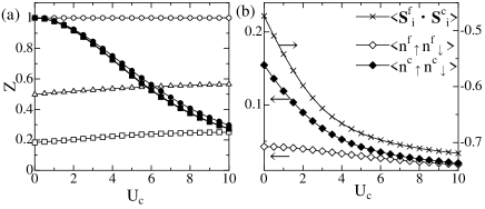
Fig.  1: (a) Renormalization factors as a function of the c-c Coulomb interaction $U_{c}$: solid (open) symbols represent $Z_{c}$ ($Z_{f}$). We show the results for $U_{f}=0.0,5.0$ and $10.0$ as circles, triangles and squares, respectively. (b) Local spin correlation function $\langle{\bf S}_{i}^{f}\cdot{\bf S}^{c}_{i}\rangle$, and double-occupation probabilities $\langle n^{f}_{\uparrow}n^{f}_{\downarrow}\rangle$ and $\langle n^{c}_{\uparrow}n^{c}_{\downarrow}\rangle$.

As shown in Fig. 1 (a), the introduction of $U_{c}$ reduces the renormalization factor $Z_{c}$, while it does not alter the factor $Z_{f}$ so much. Namely, the c-c interaction $U_{c}$ mainly renormalizes conduction electrons, as naively expected. We also show in Fig. 1 (b) the c-f spin correlation function, $\langle{\bf S}^{f}_{i}\cdot{\bf S}^{c}_{i}\rangle$, and the double-occupation probabilities, $\langle n^{f}_{\uparrow}n^{f}_{\downarrow}\rangle$ and $\langle n^{c}_{\uparrow}n^{c}_{\downarrow}\rangle$, for $f$ and conduction electrons. Introducing $U_{c}$, the double occupation probabilities of the two bands are decreased, and accordingly the c-f spin correlation function approaches -3/4, implying that the spin singlet is formed between the $f$ electron and the conduction electron. Therefore, the spin sector for large $U_{f}$ and $U_{c}$ is stabilized by the formation of the local singlet at each site.

Although the interaction $U_{c}$ enhances electron correlations, it may not necessarily reduce the spectral gap characteristic of the Kondo insulating phase. To see this clearly, we compute the density of states (DOS) for the one-particle spectrum shown in Fig. 2.

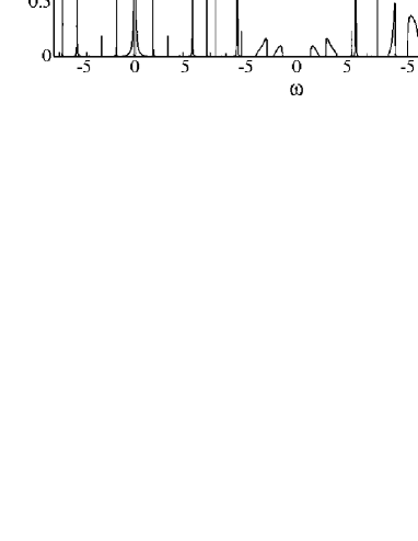
Fig.  2: DOS of $f$ electrons for the single-band PAM.

For the non-interacting case ($U_{f}=U_{c}=0$), the gap in the vicinity of the Fermi level is caused by the bare c-f hybridization. When the f-f Coulomb interaction $U_{f}$ is increased by keeping $U_{c}=0$, $f$ electrons are renormalized, resulting in the formation of the small gap typical for the Kondo insulator. In addition to the low-energy Kondo peaks, the large spectral weight appears around $\tilde{\varepsilon}_{f}$ and $\tilde{\varepsilon}_{f}+U_{f}$, which is represented by a bunch of spiky peaks since the effective heat bath is represented by a few sites in the linearized DMFT. Similar behavior to reduce the gap is observed when only the c-c Coulomb interaction $U_{c}$ is introduced, as should be expected.

On the other hand, when $U_{c}$ is turned on together with $U_{f}$, the gap is increased as shown in Fig. 2. This is contrasted to the above-mentioned cases possessing either of $U_{f}$ or $U_{c}$. To make this behavior more explicit, we plot the gap $\Delta$ in Fig. 3, from which we can indeed see the above mentioned properties.

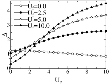
Fig.  3: Spectral gap $\Delta$ for different values of $U_{f}$ as a function of the c-c interaction $U_{c}$ among conduction electrons.

The gap is expressed in terms of the renormalization factors as

$$\Delta=-Z_{c}+\sqrt{{Z_{c}}^{2}+4Z_{c}Z_{f}V_{g}^{2}},$$ (17)

where $V_{g}\equiv V+g$ is the effective hybridization defined before. It is seen from this formula that both of $Z_{f}$ and $Z_{c}$ have a tendency to reduce the gap $\Delta$. For example, when $U_{c}=0$, the gap is decreased by $U_{f}$, leading to the Kondo insulator with a small gap $\sim 4Z_{f}V^{2}$. As mentioned above, however, the interplay of $U_{c}$ and $U_{f}$ increases the gap. We find that this enlargement is due to the c-f non-diagonal self-energy. Namely, in contrast to the simple PAM, the hybridization gap is affected not only by $Z_{f}$ and $Z_{c}$ but also by the shift in the c-f hybridization, $g$, via the relation $V_{g}=V+g$ in the formula (17). Note that $g$ is finite only in the case $U_{c}\neq 0$ and $U_{f}\neq 0$, and gives rise to the large gap in Fig. 3. In this way, the Kondo insulator is adiabatically connected to the Mott insulator realized in the case $U_{c},U_{f}>>t$, where the gap is mainly determined by $U_{f}$ or $U_{c}$. These results are consistent with those obtained by non-crossing approximation.${}^{\hbox{\immediate{?})}}$

4 Two-Orbital Periodic Anderson Model

We now move to the two-orbital PAM to clarify the role of the orbital degrees of freedom.

4.1 Correlations due to f-f interactions

We first turn off the interactions for conduction electrons, $U_{c}=U^{\prime}_{c}=J_{c}=0$, and explore how the interactions for $f$ electrons affect the formation of the Kondo insulator.

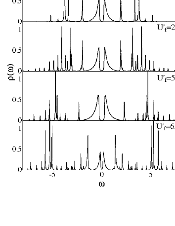
Fig.  4: DOS of $f$ electrons for different values of the inter-orbital f-f Coulomb repulsion $U_{f}^{\prime}$ with a fixed $U_{f}=5.0$.

Shown in Fig. 4 is the DOS for $f$ electrons when the inter-orbital f-f interaction $U^{\prime}_{f}$ is varied with $U_{f}=5.0$ being fixed. Increasing $U_{f}^{\prime}$, the upper and lower Hubbard-type bands, which are represented by $\delta$-function like peaks, are shifted to the higher energy region with their weight being increased. On the other hand, qualitatively different behavior emerges for the gap formation in the lower energy region. Namely, the size of the gap is once enhanced with the increase of $U_{f}^{\prime}$, but beyond $U_{f}^{\prime}\sim U_{f}$ it starts to decrease. This nonmonotonic behavior is explicitly observed in Figs. 5 (a) and (b), where the renormalization factor $Z_{f}$ and the size of the gap $\Delta$ are plotted as a function of $U_{f}^{\prime}$.

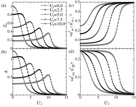
Fig.  5: (a) Renormalization factor $Z_{f}$, (b) spectral gap $\Delta$, (c) and (d) local correlation functions for $f$ electrons, as a function of the inter-orbital f-f interaction $U^{\prime}_{f}$

In the case $U_{f}=0$, $Z_{f}$ and $\Delta$ decrease monotonically with the increase of $U^{\prime}_{f}$. The resulting insulating phase is regarded as a variant of the Kondo insulator, for which enhanced orbital (instead of spin) fluctuations reduce the gap. On the other hand, as already mentioned, a finite $U_{f}$ leads to the maximum structure in $Z_{f}$ and $\Delta$ around $U^{\prime}_{f}\sim U_{f}$. Therefore, low-energy electronic properties are quite sensitive to the balance of the Coulomb interactions $U_{f}$ and $U^{\prime}_{f}$, as pointed out in a related context of the Hubbard model.${}^{\hbox{\immediate{?},\penalty 1000\hskip 0.91003pt plus 0.70004pt minus 0.70004pt{?})}}$ To confirm this, we also calculate the local correlation functions shown in Figs. 5 (c) and (d). The inter-orbital f-f interaction $U^{\prime}_{f}$ increases the double-occupation probability $\langle n^{f}_{m\uparrow}n^{f}_{m\downarrow}\rangle$ in the same orbital , while it decreases $\langle n^{f}_{1\alpha}n^{f}_{2\beta}\rangle$ for two electrons occupying different orbitals. It should be noticed that these quantities are altered dramatically around $U_{f}\sim U^{\prime}_{f}$, implying that orbital fluctuations are enhanced there. Therefore, we can say that the Kondo-insulating gap is enlarged due to orbital fluctuations among $f$ electrons.

We next consider the effects of the exchange coupling $J_{f}$ to further clarify the role of local spin and orbital degrees of freedom.

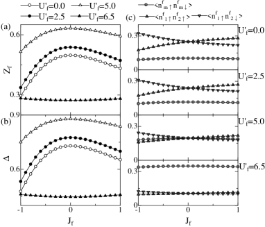
Fig.  6: (a) Renormalization factor $Z_{f}$, (b) spectral gap $\Delta$, and (c) local correlation functions as a function of the Hund coupling $J_{f}$. Other parameters are chosen as $U_{f}=10.0,U_{c}=U^{\prime}_{c}=0.0$ and $J_{c}=0.0$.

In Figs. 6 (a) and (b), we show $Z_{f}$ and $\Delta$, which exhibit analogous $J_{f}$ dependence. Since the Hund coupling restricts the available phase space of $f$ electrons at each site, it has a tendency to suppress orbital fluctuations, thereby reducing both of $Z_{f}$ and $\Delta$. Since the effective internal degrees of freedom depend on the sign of $J_{f}$, the above effects appear differently in two cases. When $J_{f}>0$, the Hund coupling favors a triplet state at each site, while the negative coupling $J_{f}(<0)$ a singlet state. Therefore, for $J_{f}<0$, orbital fluctuations are suppressed rather strongly, thus leading to a more prominent decrease in $Z_{f}$ and $\Delta$. If $U^{\prime}_{f}$ gets large, the system favors the local configuration of two electrons occupying the same orbital, so that the gap becomes insensitive to the Hund coupling in that parameter region, as seen in Figs. 6 (a) and (b).

For reference, we show the local correlation functions $\langle n^{f}_{1\uparrow}n^{f}_{2\uparrow}\rangle$ and $\langle n^{f}_{1\uparrow}n^{f}_{2\downarrow}\rangle$ in Fig. 6 (c), from which we can check to what extent the exchange coupling $J_{f}$ affects spin and orbital fluctuations. It is seen that these quantities characterize the enhancement of triplet or singlet correlations depending on the sign of $J_{f}$, but only in the region $U^{\prime}_{f}<U_{f}$. In the case $U^{\prime}_{f}>U_{f}$, however, the double occupancy of either of two orbitals is favored, and thus $\langle n^{f}_{m\uparrow}n^{f}_{m\downarrow}\rangle$ gets larger than $\langle n^{f}_{1\uparrow}n^{f}_{2\uparrow}\rangle$ and $\langle n^{f}_{1\uparrow}n^{f}_{2\downarrow}\rangle$. This implies that the Hund coupling $J_{f}$ is irrelevant in this case, consistent with the above results.

4.2 Correlations due to c-c interactions

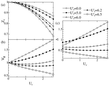
Fig.  7: (a) Renormalization factor $Z_{c}$, (b) effective hybridization $V_{g}$ and (c) spectral gap $\Delta$ as a function of the intra-orbital c-c interaction $U_{c}$ for different values of the inter-orbital f-f interaction $U^{\prime}_{f}$. The intra-orbital f-f Coulomb interaction is fixed as $U_{f}=5.0$.

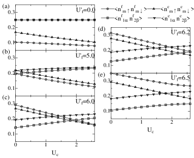
Fig.  8: Local correlation functions as a function of intra-orbital c-c interaction $U_{c}$. The parameters are chosen as in 7

We now study the influence coming from correlations among conduction electrons. In Figs. 7 and 8, several quantities discussed so far are plotted in the presence of the c-c Coulomb interaction $U_{c}$ together with f-f interactions $U_{f}$ and $U^{\prime}_{f}$. We notice that the effect of $U_{c}$ shows up differently in the cases of $U_{f}>U^{\prime}_{f}$ and $U_{f}<U^{\prime}_{f}$. For $U_{f}>U^{\prime}_{f}$, the gap $\Delta$ increases, although the renormalization factor $Z_{c}$ decreases, reflecting electron correlations among conduction electrons (Figs. 7 (a) and (c)). This behavior is somewhat similar to the case discussed in the single-orbital model in Figs. 1 and 2. Namely, the increase of the gap is caused by the increase of the hybridization $V_{g}=V+g$ due to the c-f self-energy. This is indeed confirmed in Fig. 7 (b). In this case, the system changes continuously from the Kondo insulator to the Mott insulator This is typically seen in the local correlation functions shown in Fig. 8 (a), where both of the double-occupation probabilities $\langle n^{f}_{m\uparrow}n^{f}_{m\downarrow}\rangle$ and $\langle n^{c}_{m\uparrow}n^{c}_{m\downarrow}\rangle$ are suppressed with the increase of $U_{c}$.

On the other hand, in the case of $U_{f}<U^{\prime}_{f}$, the gap $\Delta$ decreases with the increase of $U_{c}$, which is caused by the decrease of $V_{g}$. As shown in Figs. 8 (d) and (e), the double-occupation probability of the same orbital at $U_{c}=0$ is enhanced not only for $f$ electrons ($\langle n^{f}_{m\uparrow}n^{f}_{m\downarrow}\rangle$) but also for conduction electrons ($\langle n^{c}_{m\uparrow}n^{c}_{m\downarrow}\rangle$), even if $U_{c}^{\prime}=0$. This is a nontrivial effect due to the interplay of these interactions, and implies that the system at $U_{c}=0$ is a variant of the Kondo insulator, for which the strong renormalization is caused by orbital fluctuations due to the inter-orbital interactions. The increase of $U_{c}$ in turn suppresses such enhanced orbital fluctuations, as typically seen in Figs. 8 (d) and (e), and at the same time gives rise to the decrease of $V_{g}$. Therefore, we may say that the resulting insulator is still in the Kondo insulating phase with a small gap, which possesses both of the enhanced spin and orbital fluctuations.

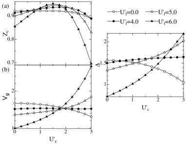
Fig.  9: (a) Renormalization factor of conduction electrons $Z_{c}$, (b) effective hybridization $V_{g}$, (c) spectral gap $\Delta$ as a function of the inter-orbital c-c Coulomb interaction $U^{\prime}_{c}$. We set $U_{f}=5.0$ and $U_{c}=2.0$ for simplicity.

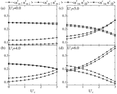
Fig.  10: Local correlation functions for $f$ and conduction electrons. We set $U_{f}=5.0$ and $U_{c}=2.0$.

We finally observe what happens when we further introduce the inter-orbital c-c Coulomb interaction $U_{c}^{\prime}$ among conduction electrons. We fix the values $U_{f}=5.0$ and $U_{c}=2.0$, and compute the gap and the renormalization factor of conduction electrons as a function of $U^{\prime}_{c}$ for various choices of $U^{\prime}_{f}$. Since we can follow the arguments outlined above, we only mention some interesting points briefly. As seen from Fig. 9, the gap is not so sensitive to the value of $U_{c}^{\prime}$ for small $U_{f}^{\prime}$. A remarkable point is that when $U_{f}^{\prime}$ is large (e.g. $U_{f}^{\prime}=6.0$), all of $Z_{c}$, $V_{g}$ and $\Delta$ change dramatically as a function of $U_{c}^{\prime}$. Although the spectral gap $\Delta$ increases similarly to the case discussed in Fig. 7 for small $U_{f}^{\prime}$, we should notice that the nature of the insulating phase is different from each other. The difference is distinguished in terms of the local correlation functions shown in Fig. 10. In particular, from panel (d) for $U_{f}^{\prime}=6.0$, we can see that $\langle n^{f}_{m\uparrow}n^{f}_{m\downarrow}\rangle$ and $\langle n^{c}_{m\uparrow}n^{c}_{m\downarrow}\rangle$ are enhanced, whereas $\langle n^{f}_{1\alpha}n^{f}_{2\beta}\rangle$ and $\langle n^{c}_{1\alpha}n^{c}_{2\beta}\rangle$ are suppressed. This implies that the insulating phase in that parameter region may be regarded as a variant of the Mott insulator with a large gap, for which orbital fluctuations are enhanced while spin fluctuations are suppressed. This phase is qualitatively different from the one discussed in Fig. 7 for small $U_{f}^{\prime}$, where spin (orbital) fluctuations are enhanced (suppressed) in the presence of $U_{c}$.

Before closing this section, brief comments are in order for the impacts due to other interactions we have not addressed here. We have refrained from discussing the effects due to the exchange coupling $J_{c}$ among conduction electrons, since they are mostly the same as those of $J_{f}$. Also, we have not argued the influence due to the c-f Coulomb repulsion in order to avoid the model to be too complicated. We have checked that this interaction has a tendency to enlarge the spectral gap.

5 Summary

We have studied electron correlations for the orbitally degenerate periodic Anderson model by means of a linearized version of dynamical mean field theory. In particular, we have focused on the role played by various intra- and inter-orbital interactions.

By taking the single orbital model, we have first demonstrated how the c-c Coulomb repulsion naturally interpolates the Kondo insulator and the Mott insulator. In this case, the c-f part of the self-energy plays a major role rather than the renormalization effects due to $Z_{c}$ and $Z_{f}$.

In the two orbital model, there are some remarkable effects, which do not appear in the single-orbital case, due to the interplay of the intra- and inter-orbital interactions. One of the most interesting results is that orbital fluctuations are enhanced around $U_{f}=U^{\prime}_{f}$, which in turn suppress the renormalization effect. As a result, the Kondo insulating gap shows a maximum around there. This effect is somehow obscured by the exchange coupling $J_{f}$ between $f$ orbitals since it has a tendency to reduce orbital fluctuations. Accordingly, the introduction of $J_{f}$ again enhances the renormalization effect, making the Kondo gap smaller.

Upon introducing the interactions for conduction electrons as well as $f$ electrons in the degenerate model, there appear a variety of remarkable effects due to the interplay of these interactions. In fact, reflecting the subtle balance of the interactions, the insulating phase with strong correlations has either the enlarged gap or the reduced gap, for which either of spin or orbital fluctuations (both of them in some cases) are enhanced.

In this paper, we have restricted our analysis to the non-magnetic phase. We have indeed observed a number of interesting properties even in such nonmagnetic insulating phase. It remains an interesting problem in the future study to clarify the competition between the nonmagnetic insulating state and magnetically ordered states, which may be particularly important in the system possessing large interactions.

References

- [1] T. Susaki et al: Phys. Rev. Lett. 77 (1996) 4269.
- [2] K. Sugiyama, F Iga, and M. Kasaya: J. Phys. Soc. Jpn. 57 (1988) 3946.
- [3] T. Saso and H. Harima: J. Phys. Soc. Jpn. 68 (1999) 2491.
- [4] J. W. Allen, B. Batlogg, and P. Wachter: Phys. Rev. B. 20 (1979) 4807.
- [5] M. F. Hundley, P. C. Canfield, and Z. Fisk: Phys. Rev. B. 42 (1990) 6842.
- [6] A. Severing, J. D. Thompson, P. C. Canfield, Z. Fisk, and P. S. Riseborough: Phys. Rev. B 44 (1991) 6832.
- [7] T. E. Mason et al: Phys. Rev. Lett. 69 (1992) 490.
- [8] P. S. Riseborough: Phys. Rev. B 45 (1992) 13984.
- [9] C. Sanchez-Castro, K. S. Bedell, and B. R. Cooper: Phys. Rev. B 47 (1993) 6879.
- [10] J. C. Cooley, M. C. Aronson, Z. Fisk, and P. C. Canfield: Phys. Rev. Lett. 74 (1995) 1629.
- [11] T. Brugger, T. Schreiner, G. Roth, P. Adelmann, and G. Czjzek: Phys. Rev. Lett. 71 (1993) 2481.
- [12] Y. M. Li: Phys. Rev. B. 52 (1995) 6979.
- [13] J. Igarashi, K. Murayama, and P. Fulde: Phys. Rev. B. 52 (1995) 15966.
- [14] K. Itai and P. Fazekas: Phys. Rev. B. 54 (1996) 752.
- [15] T. Schork and S. Blawid: Phys. Rev. B. 56 (1997) 6559.
- [16] Y. Ono, T. Matsuura, and Y. Kuroda:J. Phys. Soc. Jpn. 63 (1993) 1406.
- [17] M. Jarrell, H. Pang, D. L. Cox, F. Anders, and A. Chattopadhyay: Physica B 230-232 (1997) 557.
- [18] A. Tsuruta, A. Kobayashi, and Y. Ōno: J. Phys. Soc. Jpn. 68 (1999) 2491.
- [19] W. Metzner and D. Vollhardt: Phys. Rev. Lett. 69 (1989) 324.
- [20] E. Müller-Hartmann, Z. Phys. B: Condens. Matter 74 (1989) 507.
- [21] T. Pruschke, M. Jarrell, and J. K. Freericks: Adv. Phy. 42 (1995) 187.
- [22] A. Georges, G. Kotliar, W. Krauth, and M. J. Rozenberg: Rev. Mod. Phys 68 (1996) 13.
- [23] A. Georges and G. Kotliar: Phys. Rev. B. 45 (1992) 6479.
- [24] M. Jarrell: Phys. Rev. Lett. 69 (1992) 168.
- [25] X. Y. Zhang, M. J. Rozenberg, and G. Kotliar: Phys. Rev. Lett. 70 (1993) 1666.
- [26] M. Caffarel and W. Krauth: Phys. Rev. Lett. 72 (1994) 1545.
- [27] D. S. Fisher, G. Kotliar, and G. Moeller: Phys. Rev. B. 52 (1995) 17112.
- [28] H. Kajueter and G. Kotliar: Phys. Rev. Lett. 77 (1996) 131.
- [29] R. Bulla: Phys. Rev. Lett. 83 (1999) 136.
- [30] M. Potthoff: Phys. Rev. B. 64 (2000) 165114.
- [31] R. Bulla, and M. Potthoff: Eur. Phys. J. B. 13 (2000) 257.
- [32] Y. Ōno, R. Bulla, A. C. Hewson, and M. Potthoff: Eur. Phys. J. B. 22 (2001) 283.
- [33] M. J. Rozenberg: Phys. Rev. B. 55 (1997) R4855.
- [34] K. Held and D. Vollhardt: Euro. Phys. J. B 5 (1998) 473.
- [35] J. E. Han, M. Jarrell, and D. L. Cox: Phys. Rev. B. 58 (1998) R4199.
- [36] Th. Maier, M. B. Zölfl, Th. Pruschke, and J. Keller: Eur. Phys. J. B 19 (1999) 377.
- [37] T. Momoi and K. Kubo: Phys. Rev. B. 58 (2000) R567.
- [38] Y. Imai and N. Kawakami: J. Phys. Soc. Jpn. 70 (2001) 2365.
- [39] A. Koga, Y. Imai, and N. Kawakami: Phys. Rev. B. 66 (2002) 165107.
- [40] V. S. Oudovenko and G. Kotliar: Phys. Rev. B. 65 (2002) 0750102.
- [41] S. Florens, A. Georges, G. Kotliar, and O. Parcollet: Phys. Rev. B. 66 (2002) 205102.
- [42] Y. Ōno, M. Potthoff, and R. Bulla: Phys. Rev. B. 67 (2003) 035119.
- [43] A. Koga, T. Ohashi, Y. Imai, S. Suga and N. Kawakami: J. Phys. Soc. Jpn. 72 (2003) 1306.
- [44] A. Liebsch: Phys. Rev. Lett. 91 (2003) 226401.
- [45] A. Koga, N. Kawakami, T.M. Rice, and M. Sigrist: cond-mat/0401223.
- [46] T. Mutou and D. Hirashima: J. Phys. Soc. Jpn. 63 (1994) 4475; T. Mutou: Phys. Rev. B. 64 (2001) 165103.
- [47] M. Jarrell: Phys. Rev. B. 51 (1995) 7429.
- [48] T. Saso and M. Itoh: Phys. Rev. B. 53 (1996) 6877.
- [49] Th. Pruschke, R. Bulla, M. Jarrell: Phys. Rev. B. 61 (2000) 12799.
- [50] D. Meyer and W. Nolting: Phys. Rev. B. 61 (2000) 13465.
- [51] Chang-Il Kim, Y. Kuramoto, and T. Kasuya: J. Phys. Soc. Jpn. 59 (1990) 2414.