Quantum Monte Carlo simulations of confined bosonic atoms in optical lattices

Abstract

We study properties of ultra-cold bosonic atoms in one, two and three dimensional optical lattices by large scale quantum Monte Carlo simulations of the Bose Hubbard model in parabolic confinement potentials. Local phase structures of the atoms are shown to be accessible via a well defined local compressibility, quantifying a global response of the system to a local perturbation. An indicator for the presence of extended Mott plateaux is shown to stem from the shape of the coherent component of the momentum distribution function, amenable to experimental detection. Additional fine structures in the momentum distribution are found to appear unrelated to the local phase structure, disproving previous claims. We discuss limitations of local potential approximations for confined Bose gases, and the absence of quantum criticality and critical slowing down in parabolic confinement potentials, thus accounting for the fast dynamics in establishing phase coherence in current experiments. In contrast, we find that flat confinement potentials allow quantum critical behavior to be observed already on moderately sized optical lattices. Our results furthermore demonstrate, that the experimental detection of the Mott transition would be significantly eased in flat confinement potentials.

I Introduction

Experiments on ultra cold atomic gases in optical lattices greiner ; esslinger provide the unique opportunity to directly compare theoretical studies of strongly correlated many body quantum lattice models with near-perfect experimental realizations of those models zoller . Unlike for other strongly correlated systems, where often the models simulated numerically are prototype toy models for describing the properties of such materials, the same models are here realistic models of confined cold atoms, allowing for quantitative comparisons.

So far, experiments have focused on bosonic atoms greiner ; esslinger , which are easier to cool than fermions. A quantitative understanding of these bosonic systems will, in the future, allow to correctly interpret measurements on atomic fermion gases, which could be used as analog quantum simulators for strongly correlated fermionic systems hofstetter .

Here we present results of an extensive set of quantum Monte Carlo simulations performed on one dimensional (1D), two dimensional (2D) and three dimensional (3D) systems of confined bosonic atoms in optical lattices, extending previous work in 1D batrouni and 3D prokofev . Parts of our results were already presented elsewhere advances , here we provide a more detailed discussion and new results on confined Bose gases. Details on the many body quantum lattice model used for simulating confined bosons, as well as the employed quantum Monte Carlo method are discussed in the following section.

In the first part of the paper, Sec. II, we focus on simulations of bosons in 2D confinement potentials, and study various aspects of confined bosons in a realistic setup. In particular, we (i) identify a local probe for the state at a given location inside the inhomogeneous trap, (ii) present a detailed analysis concerning the limitations of local potential approximations, and (iii) discuss the nature of spatial correlations inside the trap.

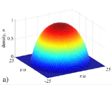
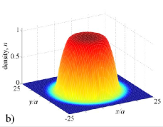
Figure 1: Spatial dependence of the local density for two dimensional confined atomic boson systems: a) in the superfluid phase; b) at stronger lattice depths a central Mott insulating region is formed. The simulations were performed for a parabolic trap with curvature $V/U=0.002$, at $\mu/U=0.37$, for $U/t=6.7$ (a), and $U/t=25$ (b).

Next, in Sec. IV, we introduce an effective model describing the inhomogeneous Bose gas inside the confinement potential. This allows us to study the finite size effects arising from the limited extent of the Bose gas in the trap. Using this effective model, we discuss the absence of quantum critical behavior for bosons trapped in confinement potentials.

In a third part, Sec. V, we aim at identifying experimentally accessible quantities that signal restructurings in the density distribution of the confined Bose gases. For this purpose, we monitor the evolution of the momentum distribution function upon increasing the lattice depth of the optical lattice, similar to the experimental procedure greiner . We find that a method put forward recently prokofev for identifying the phase structure of the confined Bose gas is not appropriate. However, by monitoring the evolution of both the coherence fraction and the full width at half maximum of the coherent part of the momentum distribution function we obtain clear signals for restructurings of the density distributions. Finally, we summarize our observations in Sec. VI, along with implications for the experiments in confined atom systems.

II Model and numerical techniques

Cold confined atomic Bose gases in an optical lattice are direct experimental realizations of the inhomogeneous Bose Hubbard Hamiltonian zoller

$$H = -t\sum_{\langle i,j\rangle}\left(b^{\dagger}_{i}b_{j}+h.c.\right)$$

$$+\frac{U}{2}\sum_{i}n_{i}(n_{i}-1)+V\sum_{i}r^{2}_{i}n_{i}-\mu\sum_{i}n_{i},$$

where $b^{\dagger}_{i},(b_{i})$ denotes the creation (destruction) operator for bosons at lattice site $i$, located a distance $r_{i}$ from the center of the trap, and $n_{i}=b^{\dagger}_{i}b_{i}$ the local density operator. The nearest neighbor hopping integral $t$, the onsite Hubbard repulsion $U$ , and the curvature of the parabolic confinement potential $V>0$ are tunable parameters in experiments.

After evaporative cooling of the atoms, the experiments are, to a good approximation, performed at constant particle number. Similarly, the chemical potential $\mu$ allows us to control the filling of the trap in the numerical simulations. For the discussions below we introduce a local chemical potential

$$\mu^{\rm eff}_{i}=\mu-Vr^{2}_{i}$$ (2)

which decreases upon moving away from the trap center.

Quantum Monte Carlo (QMC) simulations of the Hamiltonian Eq. (II) were performed using the Stochastic Series Expansion method sse ; loopoperator , with directed loop updates sylju1 ; sylju2 ; alet . This algorithm requires a cutoff $N_{\rm max}$ on the local site occupation. Performing simulations at mean densities $\langle n_{i}\rangle\leq 1$, a cutoff $N_{\rm max}=2$ or $3$ can be chosen without introducing significant errors. The temperature used in the QMC calculations was chosen low enough to be essentially in the ground state.

All lengths are set in units of the lattice constant $a$, and the simulation box is taken large enough, to ensure that outside its boundary the local density $n_{i}$ vanishes due to depopulation by large negative values of $\mu^{\rm eff}_{i}$. For the values chosen in our simulations we needed to keep up to 500-site chains in 1D, $50\times 50$ square lattices in 2D and up to $16^{3}$-site cubes in 3D.

To distinguish the local phases in the inhomogeneous system and to probe for quantum criticality we define the local compressibility at site $i$,

$$\kappa^{\rm local}_{i}=\left\langle\frac{\partial n}{\partial\mu^{\rm eff}_{i}}\right\rangle=\beta\left(\langle n_{i}n\rangle-\langle n_{i}\rangle\langle n\rangle\right),$$ (3)

by the response of the system’s density, n, to a local chemical potential change at site $i$. Here, $\beta=1/T$ denotes the inverse temperature. Another way of probing for local properties is to measure local density fluctuations batrouni . These are related, by

$$\Delta_{i}=\frac{1}{\beta}\left\langle\frac{\partial n_{i}}{\partial\mu^{\rm eff}_{i}}\right\rangle=\langle n_{i}^{2}\rangle-\langle n_{i}\rangle^{2},$$ (4)

to a local density response. In the homogenous case, the global compressibility

$$\kappa=\left\langle\frac{\partial n}{\partial\mu}\right\rangle=\beta\left(\langle n^{2}\rangle-\langle n\rangle^{2}\right)$$ (5)

is equal to the local comressibility $\kappa^{\rm local}_{i}$ defined in Eq. (3) at each lattice site $i$, but is in general not given by $\beta\Delta_{i}$. This is due to correlations between different lattice sites in the superfluid regime. Only in the Mott-insulating phases of the homogenous system, where these correlations are absent, do all quantities become zero. We will show in Sec. III.2 that the local compressibility, $\kappa^{\rm local}$, as defined in Eq. (3) is indeed able to characterize the local state near a given site even in the inhomogenous case.

In addition to measuring local quantities, we measure the momentum distribution function,

$$n({\bf k})=\frac{1}{N}\sum_{i,j}e^{i({\bf r}_{i}-{\bf r}_{j}){\bf k}}\langle b^{\dagger}_{i}b_{j}\rangle,$$ (6)

where $N$ denotes the total number of particles within the system. This way the momentum distribution is normalized to unity, and the coherence fraction given by the height of the coherence peak, $n({\bf k}=0)$.

The momentum distribution function $n({\bf k})$ is directly accessible in experimental studies of confined atomic gases. For negligible interparticle interactions during ballistic expansion of the atomic cloud, it essentially maps onto the interference pattern of the resulting absorption imagines roth . Due to the tight binding approximation of the Bose-Hubbard model, the numerical momentum distribution functions are periodic in the extended zone scheme. A finite extent of the Wannier functions on each site in an optical lattice leads to a form factor in the momentum distribution prokofev , resulting in unequal heights of the higher order Bragg peaks, as observed in the experimental interference patterns greiner .

To further quantify spatial correlations within the trap, we measure the one particle density matrix, i.e. the correlation function

$$g(i,j)=\langle b^{\dagger}_{i}b_{j}\rangle,$$ (7)

between bosons on lattice sites $i$ and $j$.

III Simulations of realistic 2D traps

III.1 Phase coexistence in trapped systems

Trapped inhomogeneous systems can show coexistence of both superfluid and Mott insulating regions, as has been clearly identified in experiments greiner ; esslinger , in mean field investigations zoller , numercial renormalization group pollet and Gutzwiller ansatz calculations schroll and in numerical simulations in 1D batrouni ; kollath ; bergkvist and 3D prokofev . Simulating large realistic systems in 2D, we can clearly observe this coexistence. For large hoppings $t$ the total system is superfluid (Fig. 1a).

As the hopping amplitude $t$ is decreased, a Mott insulating plateau with integer density (here $\langle n_{i}\rangle=1$) forms in the center of the trap, as seen in Fig. 1b. A superfluid ring-like region with a non-uniform particle density surrounds the central plateau. The typical width of this superfluid ring is $6-8$ times the lattice unit, for the parameters used in our simulations. Far away from the center, the density is $\langle n_{i}\rangle=0$ which can also be viewed as a Mott plateau.

The emergence of the Mott plateau and the shrinking of the superfluid region have been interpreted as a quantum phase transition greiner . We prefer to view it as a crossover where the volume fraction of the Mott insulating phase grows and that of the superfluid phase shrinks. After discussing the quantitative properties of the two phases and of the boundary region we will, in Sec. IV.3, show that no quantum critical behavior is observed in this system, which supports our interpretation of this phenomenon as a crossover instead of a phase transition.

III.2 Local compressibility

Fig. 1 is useful for a qualitative view, but we need a quantitative probe to distinguish the different phases. This probe is given by the compressibility. QMC results for the local compressibility within the trap of Fig. 1b are shown in Fig. 2. The extent of the superfluid shell is clearly reflected by this local probe, which also shows that the compressibility is largest close to the outer regions of the superfluid shell.

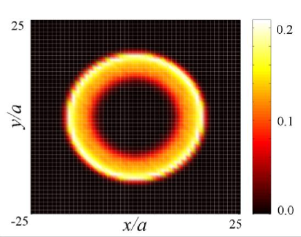
Figure 2: Spatial dependence of the local compressibility, $\kappa^{\rm local}$, of bosons in a two dimensional parabolic trap with curvature $V/U=0.002$, for $\mu/U=0.37$ and $U/t=25$. A superfluid ring surrounding the $n=1$ central Mott plateau is clearly resolved.

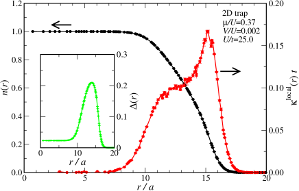
Figure 3: Radial dependence of the density, $n$, and local compressibility, $\kappa^{\rm local}$, of bosons in a two dimensional parabolic trap with curvature $V/U=0.002$, for $\mu/U=0.37$ and $U/t=25$, with a superfluid ring surrounding the $n=1$ central Mott plateau. The inset shows the radial dependence of the local density fluctuations, $\Delta$, which remain finite within the Mott plateau region.

For a quantitative analysis we plot in Fig. 3 the radial dependence of both the local density $n(r)$ and the local compressibility $\kappa^{\rm local}(r)$ as a function of the distance $r$ from the center of the trap. We observe two well defined Mott regions with local density $n(r)=1$ and $n(r)=0$. In these Mott plateaux, the local compressibility vanishes, whereas it is finite in the intervening superfluid ring with non-integral density $0<n(r)<1$.

More precisely, we observe two well defined peaks in $\kappa^{\rm local}(r)$, signaling an increase in the particle number fluctuations at the boundaries to the Mott regions. While these two peaks would be of the same height in hard-core boson models (due to particle-hole symmetry), they are asymmetric in the soft-core case.

The inset of Fig. 3 shows the radial dependence of the local density fluctuations of Eq. (4), $\Delta(r)$, first used in simulations of 1D confined Bose systems batrouni . As opposed to $\kappa^{\rm local}(r)$, this quantity peaks in the middle of the superfluid ring, and does not vanish in the central Mott plateau region. While density fluctuations are therefore most pronounced in the middle of in the superfluid, they remain finite inside the Mott plateau, due to the surrounding superfluid. These results demonstrate that the local compressibility $\kappa^{\rm local}(r)$ is a better probe for the existence of superfluid or Mott regions in the system than the onsite response expressed by $\Delta(r)$. Moreover, the response of the total system to a local excitation should be easier to study experimentally than the local response to a local excitation (for example by changing the laser intensity at one specific point).

III.3 Spatial correlations in the superfluid

In order to gain a better understanding of the extended superfluid ring, we study the behavior of the one particle density matrix, Eq. (7), in the trapped system. In Fig. 4, the spatial dependence of $g(i,j)$ is shown for a fixed site $j$, well inside the superfluid ring, and all other sites $i$ in the parabolic trap. The rapid decay of the correlations towards both the central Mott plateau region and the outside clearly exhibits the ring-like structure of the coherent superfluid.

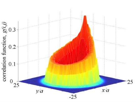
Figure 4: Spatial dependence of the correlation function $g(i,j)=\langle b^{\dagger}_{i}b_{j}\rangle$ between bosons at site ${\bf r}_{j}=(12.3,0)$ inside the superfluid shell, and all other sites $i$ within a two dimensional parabolic trap with curvature $V/U=0.002$, at $\mu/U=0.37$ and $U/t=25$.

Inside the superfluid ring the correlation function decays less rapidly. In order to make a quantitative analysis of its long distance behavior, we plot in Fig. 5 the dependence of the correlation function $g(i,j)$ for site $i,j$ along the ring on the distance $d$ between the sites, as measured along the ring. See the left inset of Fig. 5 for an illustration. We find all data for distances $d/a>5$ to follow very closely a finite size exponential decay,

$$g(d)=c+b\cosh\left(\frac{\pi r-d}{\xi}\right),$$ (8)

with a correlation length $\xi/a=21.6\pm 0.4$, and a finite constant $c=0.033\pm 0.003$. Thus, the superfluid ring does not exhibit quasi-long ranged correlations, as might have been expected from the reduced dimensionality of the quasi-1D superfluid ring. Instead, we find the ring to be wide enough for long range order, i.e. 2D behavior, to persist inside the superfluid in spite of the presence of a central Mott plateau.

A rapid decrease of the correlations, as one moves away from the middle of the superfluid, can be seen from the right inset of Fig. 5, which shows the radial dependence of the correlation function $g(d)$ at the largest distance $d=\pi r$. The correlations are thus most pronounced near $r\approx 12$, which corresponds to the central region of the superfluid ring, and become suppressed as one moves towards either boundaries. Finally, inside the Mott plateau region, the correlations are merely short ranged. Even though the coherent part of the Bose gas is thus confined to a 1D ring-like structure, the spatial dependence of the correlations inside the ring clearly exhibit the underlying 2D structure of the trapping potential.

Our findings are related to recent results in 1D systems rigol04 ; kollath , which show that the presence of a Mott insulating region does not change the long distance behavior of the one particle density matrix in trapped boson systems. Similar analysis might also apply to 3D confinement potentials, which would allow for extended 2D superfluid shells surrounding a Mott insulating central region.

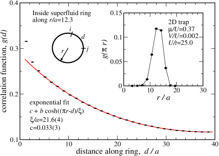
Figure 5: Dependence of the correlation function $g(d)=\langle b^{\dagger}_{i}b_{j}\rangle$ on the distance $d$ between sites $i$ and $j$ along the superfluid ring for sites within $r/a=12.3\pm 1.2$ lattice units from the center of a two dimensional parabolic trap with curvature $V/U=0.002$, at $\mu/U=0.37$ and $U/t=25$. For $d/a>5$ the data fit well ($\chi^{2}=1.6$) to an exponential decay, with a finite value of $c=0.033\pm 0.003$, and correlation length $\xi/a=21.6\pm 0.4$. The right inset shows the correlation at the largest distance, $g(\pi r)$, as a function of the distance $r$ from the trap center. The left inset illustrates the distance $d$ between two sites $i,j$ along a ring of radius $r$ employed here.

III.4 Local potential approximation

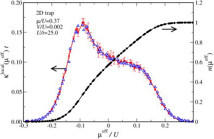
Figure 6: Local density, $n$, and local compressibility, $\kappa^{\rm local}$, of bosons in a two dimensional parabolic trap with curvature $V/U=0.002$, at $\mu/U=0.37$ and $U/t=25$, as functions of $\mu^{\rm eff}$. The results for $\kappa^{\rm local}$ from the density fluctuations, Eq.( 3) (circles) agree with the numerical derivative $\partial n/\partial\mu^{\rm eff}$ (triangles).

The confinement potential $V$ enters the Bose Hubbard Hamiltonian, Eq. (II), by coupling to the boson density. It therefore corresponds to a local chemical potential shift, expressed by the local chemical potential $\mu^{\rm eff}$, defined in Eq. (2). In Fig. 6, we show the behavior of both the local density and compressibility as functions of this effective chemical potential, $\mu^{\rm eff}$. The observed data collapse in both quantities, as well as the smooth behavior of these curves for all points on the lattice, indicate that for the realistic parameters used for the simulation, a local potential approximation holds, i.e. the local density can be determined from the value of the local chemical potential. The validity of this approximation is further confirmed by observing that the local compressibility coincides perfectly with the numerical derivative of the curve $n(\mu^{\rm eff})$, i.e.

$$\frac{\partial\langle n\rangle}{\partial\mu^{\rm eff}_{i}}=\frac{\partial\langle n_{i}\rangle}{\partial\mu_{0}}.$$ (9)

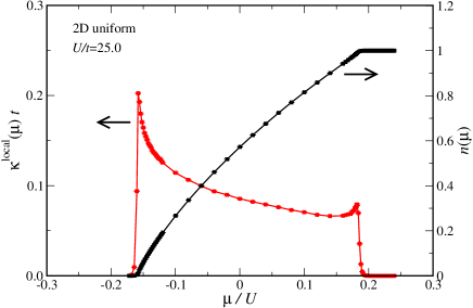
Figure 7: Density, $n$, and compressibility $\kappa$ of the Bose-Hubbard model on the 2D square lattice for $U/t=25$, as a function of $\mu$. The data are taken from simulations on a $24\times 24$ sites square lattice.

It is important to note, that $n(\mu^{\rm eff})$ is not a universal function, but depends on both the confinement geometry as well as the trap curvature, $V$. Universal behavior is violated in particular near the boundary of the superfluid, where $n(\mu^{\rm eff})$ does not behave as $n(\mu)$ for uniform systems, corresponding to $V=0$. For example, in the uniform 2D case a cusp develops when $n$ approaches $1$, as seen in Fig. 7, due to quantum criticality. This cups is absent in the confined system, where $n$ approaches $1$ rather smoothly (c.f. Fig. 6). While a local potential approximation in terms of an effective local chemical potential holds, the value of $n(\mu^{\rm eff})$ thus has to be taken from simulations in a trap, and not from the uniform system on the underlying lattice. Approximative schemes such as those of Ref. oliva , which assume that locally the system can be mapped onto an unconfined system at the local value of $\mu^{\rm eff}$, have to be applied with care. Being reasonable in the bulk of both the superfluid and the Mott plateau region, such approaches become unreliable near the interfaces between superfluid and Mott insulating regions, where differences between the confined and unconfined case are most pronounced. There QMC simulations are needed in order to obtain $n(\mu^{\rm eff})$ for a given trap geometry.

IV Thermodynamic limits and quantum criticality

In the previous section we found that in the boundary layer between Mott plateaux and superfluid regions, the confined system does not show cusps in the density profile like the uniform system does as a function of $\mu$ near the quantum critical points. This is indication for the absence of quantum criticality in the confined system. It could be argued that this is simply due to finite size effects, but here we show that the situation is indeed more subtle. For this purpose, we introduce an effective ladder model for bosons inside inhomogeneous potentials.

IV.1 Effective ladder model for the superfluid ring

A parabolic potential imposed on a regular hyper-cubic lattice makes for an irregular form of the superfluid ring surrounding the Mott insulator (see Fig. 8a). We thus first investigate whether this structural quenching is the reason for the apparent absence of quantum critical features by looking at a “smoother” lattice. Although it cannot be realized in experiments, we consider a polar lattice, such as depicted in Fig. 8, which is topologically equivalent to the ladder system in Fig. 8. The rotational invariance of the polar lattice (translation invariance of the ladders along the leg direction) simplifies the detection of critical behavior by reducing finite size effects.

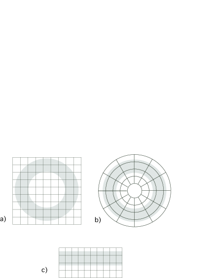
Figure 8: Different lattice topologies and expected superfluid regions (denoted in grey) for a quadratic confining potential for such topologies: (a) square lattice, (b) polar lattice, (c) ladder lattice.

While the polar and ladder lattices are not topologically equivalent to the square lattice, universality of quantum critical behavior ensures that we study the same effects. Comparing the lattices will be a further check for the validity of a local potential approximation for the confined system.

The Hamiltonian of the ladder system of size $L_{x}\times L_{y}$ is

$$H = -t\sum_{i=1}^{L_{x}}\sum_{j=1}^{L_{y}}\left(b^{\dagger}_{i,j}b_{i+1,j}+b^{\dagger}_{i,j}b_{i,j+1}+h.c.\right)$$

$$+\frac{U}{2}\sum_{i=1}^{L_{x}}\sum_{j=1}^{L_{y}}n_{i,j}(n_{i,j}-1)-\sum_{j=1}^{L_{y}}\mu(j)\sum_{i=1}^{Lx}n_{i,j},$$

where the confinement potential is now given by a chemical potential $\mu(j)$ which is constant for each leg $j$ of the ladder. The boundary conditions are chosen to be periodic along the legs of the ladder, and open in the transverse direction.

With these choices, the local density $\langle n_{i,j}\rangle$ is independent of $i$ due to translation invariance along a leg of the ladder, and we denote by $n(j)$ the density of particles on the $j$-th leg. Similarly, the local compressibility $\kappa^{\rm local}(j)$ is the same for all sites on the $j$-th leg. The results shown below have been obtained for a geometry with $L_{x}=64$, and $L_{y}=10$.

To simplify simulations, we linearize the quadratic potential, $\mu+Vj^{2}$ and set

$$\mu(j)=\mu_{0}+j\Delta\mu,$$ (11)

where $\Delta\mu$ is the difference in chemical potential between two neighboring legs. In our simulations we fix $\Delta\mu/U=0.053$ and make sure that the first leg is always in the $\langle n\rangle=0$ Mott insulating phase and the last leg in the $\langle n\rangle=1$ insulating phase. Sweeping the value of the global $\mu_{0}$ allows us to obtain results for all values of the local chemical potentials, and to drive one of the legs across the transition from the superfluid to the Mott insulating phase. We note, that a similar construction is obtained for 3D traps, by modeling the superfluid shell as a set of coupled planes with a chemical potential gradient applied perpendicular to the planes.

IV.2 Results of the ladder model and comparison to the realistic trap

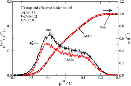
Figure 9: Local density, $n$, and local compressibility, $\kappa^{\rm local}$, for a two dimensional parabolic trap on a square lattice and for a ladder, as functions of $\mu^{\rm eff}$. The parameters for the trapping potential are $V/U=0.002$, at $\mu/U=0.37$, and the parameters of the ladder model are chosen as to cover the whole superfluid region (see text). The density profile within the trap and the ladder coincide almost perfectly. Small differences are exhibited by the two different compressibility curves, which nevertheless share the same overall shape.

In Fig. 9 we show the combined results of all simulations with different values of $\mu_{0}$. We plot both the local density $\langle n(j)\rangle$ and local compressibility $\kappa^{\rm local}(j)$ for all legs and all values of $\mu_{0}$ as functions of the local chemical potential. Note that all data from simulations using different values of $\mu_{0}$ collapse onto a single curve. Due to the equivalence of all sites on the ladder with the same value of the chemical potential, this data collapse is expected in the ladder model, where changing $\mu_{0}$ by an amount of $\Delta\mu$ corresponds to a shift in the index of each chain in the ladder.

Fig. 9 also shows the results obtained for the realistic trap, as described in the previous section. Both results coincide almost perfectly, which is a strong justification for the validity of the effective model and the applicability of a local potential approximation.

The small differences can be attributed to the different shape of the trapping potential which is parabolic for the realistic trap, but linearized in the ladder model. While differences in the densities are small, the compressibility, which is the derivative of the density, is more sensitive, marking the lack of universality.

In particular, we find that the ladder model does not show cusp-like features in the boundary regions between the superfluid and the Mott plateaux, similar to the realistic 2D trap. We thus conclude, that structural quenching in the rotational symmetric trap on the square lattice is not the reason for the apparent absence of quantum criticality since similar behavior is also found on the polar lattice, i.e. in the ladder model. We expect similar features also to be obtained for 3D traps using the effective multilayer model.

IV.3 Quantum criticality

Having shown that the ladder model captures important features of the realistic trap even quantitatively, we now discuss possible quantum criticality in confined systems.

Performing the thermodynamic limit in the uniform case does not change the model parameters apart from increasing the number of lattice sites. On the other hand, standard thermodynamic limit definitions for the confined case damle ; muramatsu imply a decrease in the trapping potential’s curvature $V$, such that

$$N\rightarrow\infty,\quad{\rm with}\quad N\sqrt{V/t}={\rm const.}$$ (12)

Such a procedure locally drives the system towards the uniform regime, since for lattice sites with a given value of $\mu^{\rm eff}$, the gradient in the confinement potential eventually becomes irrelevant on the scale set by the correlation length in their neighborhood. Therefore, the state of the uniform system at the value of $\mu^{\rm eff}$ is established there damle .

An example of this approach to the uniform system upon decreasing the trapping potential $V$ is given in Fig. 10. It shows the density $n$ as a function of $\mu^{\rm eff}$ for two different 1D traps. In the 1D case, we can study larger systems than in 2D, allowing us to decrease $V$ by a factor of $25$, which requires increasing the linear system size by a factor of $5$. While in both traps in Fig. 10 the value of the local density follows the curve $n(\mu)$ of the uniform 1D system, deviations are visible in the insets, which focus on the regions close to the Mott plateaux. In the case of the shallow trap, these deviations are clearly reduced, with more pronounced singularities developing at the critical point.

The thermodynamic limiting procedure in Eq. (12) corresponds to the limit $\Delta\mu\rightarrow 0$ in the gradient of the effective ladder model. In this limit, we recover the Bose Hubbard model on the 2D square lattice, showing 2D quantum critical behavior. A finite gradient $\Delta\mu$ in the ladder model restricts the correlation length perpendicular to the chains, and does not allow for 2D quantum critical behavior to be observed.

However, in the opposite limit, $\Delta\mu\rightarrow\infty$, we recover a 1D chain on the lowest leg, which will show 1D critical behavior. In the inset of Fig. 11 the compressibility of the Bose Hubbard model is shown on a chain of 64 sites. Already on such a short chain sharp peaks near the transition are visible, which diverge with increasing chain length batrouni_kappa .

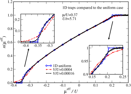
Figure 10: Local density, $n$, for bosons confined in one dimensional parabolic confinement potentials of different curvatures $V$, as a function of $\mu^{\rm eff}$. For comparison, the behavior of the density as a function of $\mu$ in the uniform 1D system is also shown. The insets focus on the regions close to $n=0$ and $n=1$, where differences between the trapped case and the uniform case are most pronounced.

One might expect this 1D quantum criticality to persist in the ladder model with a finite gradient $\Delta\mu$, observed upon changing the chemical potential $\mu_{0}$ to drive one of the legs across the phase transition. This is however not the case: While the broad peaks in Fig. 9 are weak remnants of 1D quantum criticality, they do not diverge as the size of the ladder model is increased. This is seen from Fig. 11, which shows the density and local compressibility as functions of $\mu^{\rm eff}$ for ladders of different lengths.

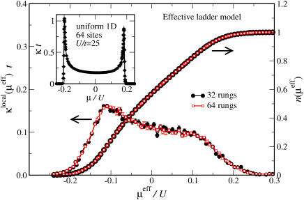
Figure 11: Local density, $n$, and local compressibility, $\kappa^{\rm local}$, for the Bose Hubbard model on ladders with different lengths as a function of $\mu^{\rm eff}$. The other parameters of the ladder model are chosen as in Fig. 9. The inset shows the compressibility for the uniform 1D case as a function of $\mu$ for a chain with 64 sites, for the same value of $U/t$ as used in the ladder model.

Therefore, the effective ladder model as well as the realistic trapped system do not show quantum criticality. The quantum critical behavior that might have been expected to occur in the boundary layer between the Mott insulator and the superfluid is destroyed by the finite gradient in the effective chemical potential, and the coupling of this layer to the rest of the system. The absence of quantum criticality in the realistic 2D parabolic trap is not only due to its finite size, but is in fact imposed by the inhomogeneity of the confinement potential, as we showed using the effective ladder description. The Mott transition observed in experiments on ultra-cold atoms greiner should not be viewed as a quantum phase transition, but instead as a crossover with changing volume fractions of the Mott plateaux and superfluid regions.

In contrast, for flat confinement potentials, corresponding to $V=0$, quantum critical behavior can be observed already on moderate system sizes. For example, the data shown in Fig. 7 for a $24\times 24$ sites 2D system, and in the inset of Fig. 11, for a 64 sites chain, both clearly reflect the quantum criticality of the uniform 2D and 1D cases.

V Identifying Mott plateau formation in traps

While measuring the spatial density distribution and the local compressibility in QMC simulations allows for the identification of the different regions inside the trap, such a local probe is not (yet) available experimentally.

In order to identify changes in the density distribution inside the trap upon varying control parameters such as $V$, $U$, or $t$, different strategies have been proposed. In particular, in Ref. prokofev it was claimed that the presence of a Mott plateau in the trap center is signaled by fine structures in the momentum distribution function, and that these are absent in traps without Mott plateaux.

Two of the configurations of Ref. prokofev are shown in Figs. 12 and 13. Here, we simulated 3D systems in a trap and used the parameters given in Ref. prokofev , and plot the resulting momentum distribution along the line from ${\bf k}=(0,0,0)$ to $(\pi/a,0,0)$, along the $k_{x}$-axis of momentum space.

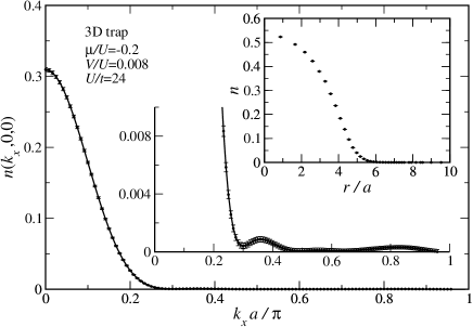
Figure 12: Momentum distribution function of bosons in a three dimensional parabolic trap with curvature $V/U=0.008$, along the line $(0,0,0)$-$(\pi/a,0,0)$ in momentum space, for $\mu/U=-0.2$, and $U/t=24$, values taken from Ref. prokofev . The lower inset exhibits the presence of satellite peaks in this system, without a Mott plateau, as seen from the radial density distribution shown in the top inset.

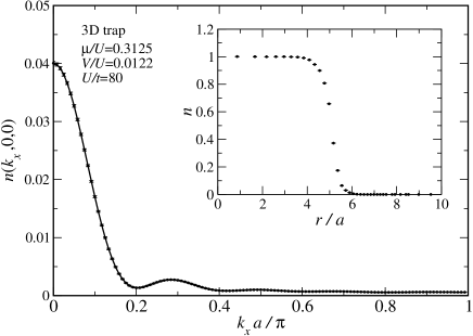
Figure 13: Momentum distribution function of bosons in a three dimensional parabolic trap with curvature $V/U=0.0122$, along the line $(0,0,0)$-$(\pi/a,0,0)$ in momentum space, for $\mu/U=-0.3125$, and $U/t=80$, values taken from Ref. prokofev . The corresponding radial density distribution is shown in the inset.

While in Fig. 13, where an extended Mott plateau is present, additional fine structures in $n({\bf k})$ are visible, such structures seem not to exist at first sight for the data shown in Fig. 12. However, similar fine structures are also present there, even on a similar scale, as clearly seen from the bottom inset of Fig. 12, which focuses on the tail of the momentum distribution function. These fine structures become invisible on the scale used for the main part of Fig. 12, due to the presence of a dominant coherence peak. We found in the simulations discussed below, that a simple correspondence as proposed in Ref. prokofev does not hold: The presence of fine structures is due to the finite extent of the superfluid within the trap, and emerges also without a Mott plateau being present in the trap center. Denoting the radial extent of the superfluid by $R$, these peaks appear for $k_{x}$ near integer multiplies of $2\pi/R$, if not masked by the incoherent background, or rendered almost invisible on the scale of the coherence peak.

For a more systematic analysis of the experimentally accessible momentum distribution function we monitor its evolution upon varying experimentally accessible control parameters of the system. We have performed sets of simulations, which mimic the experimental procedure of increasing the lattice depth of the optical lattice greiner , by reducing the hopping parameter $t$, while keeping all other parameters constant. We performed such scans for traps of different dimensionalities, and begin our discussion of the results for the 2D case.

V.1 Homogeneous and closed box 2D systems

In order to better interpret data obtained for inhomogeneous traps, we first consider the homogeneous case. To this end, we set the trap curvature $V=0$, using periodic boundary conditions (PBC), and also consider a finite square lattice with open boundary conditions (OBC), representing an infinitely sharp trapping potential, i.e. a closed box system. We then compare both the closed box and the parabolic trap to the uniform case.

The phase diagram of the Bose Hubbard model on the square lattice in the parameter regime of interest is shown in the inset of Fig. 14. While the overall phase structure is well described by mean field theory fisher ; monien , the maximum extent of the first Mott lobe of $U/t=23.3$ is thereby overestimated by about 32% of the value obtained by a strong coupling expansion ($U/t=17.54$) monien ; freericks . Thus, in order to compare later the onset of Mott plateau formation in confined systems with the homogeneous case, we first need to determine the precise phase boundary within the region of interest.

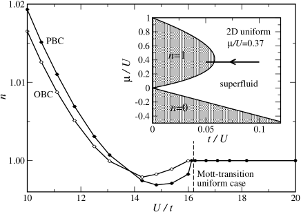
Figure 14: Density $n$ as a function of $U/t$ for bosons along a constant $\mu/U=0.37$ scan, for both periodic (PBC) and open (OBC) boundary conditions on a 24$\times$24 sites square lattice, OBC corresponding to an infinitely sharp trapping potential. The Mott transition in the uniform case is indicated by the dashed line. The inset locates this constant $\mu$ scan within the phase diagram of the uniform system.

In the following we consider a path through the phase diagram along a line of constant $\mu/U=0.37$, indicated by the directed line in the inset of Fig. 14. Moving along this line through the quantum phase transition, the system undergoes the generic transition fisher which is mean field in nature. The transition does not cross over to the special case of the commensurate transition, belonging to the $3D$ $XY$ universality class fisher .

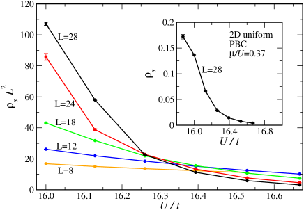
Figure 15: Scaling plot of the stiffness, $\rho_{s}$, for the Bose Hubbard model on the square lattice for periodic boundary conditions, while tuning along a constant $\mu/U=0.37$ scan. The inset shows the stiffness, $\rho_{s}$, for a $28\times 28$ sites system as a function of $U/t$.

In order to identify the Mott transition point along this scan we measured the stiffness, $\rho_{s}$, which quantifies the response of the system to a twist in the boundary conditions along the real space directions. This quantity can be calculated in QMC from the boson winding number fluctuations winding . At the quantum critical point finite size scaling theory fisher predicts it to scale in two dimensions as $L^{-z}$, where $z=2$ is the dynamical critical exponent for the generic transition, and $L$ the linear system size of a $N=L^{2}$ sites system.

The inset of Fig. 15 shows $\rho_{s}$ as a function of the inverse hopping, $U/t$, for a system of linear size $L=28$, indicating its increase upon entering the superfluid phase. The main part of Fig. 15 is a scaling plot of $\rho_{s}L^{2}$ vs. $U/t$, from which the critical point $U/t=16.25\pm 0.1$ is obtained with sufficient precision for the purpose of this study. Note that corrections to scaling are visible already at $L=12$, in agreement with a recent study, indicating that large systems sizes are needed for high precision determinations of the critical point aletgeneric . Mean field theory monien predicts a value of $U/t=23.5$ which is too large by more than 40%. Thus in 2D, corrections to mean field have to be accounted for already the uniform case.

Having established the position of the Mott transition in the uniform case, we show in Fig. 14 the evolution of the density, $n$, in homogeneous systems with PBC and OBC along the constant $\mu$ scan shown in the inset of Fig. 14. Here, we show data on systems with $24\times 24$ lattice sites. In both cases the onset of the Mott insulating regime is located close to the critical point obtained from finite size scaling. Thus already for this moderate system size, the Mott transition is located rather close to the value in the thermodynamic limit.

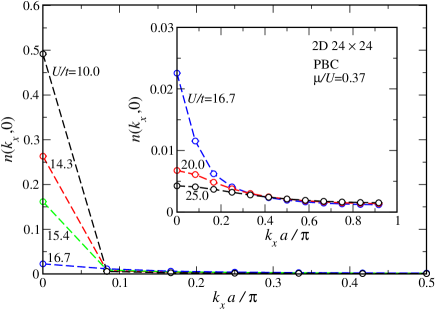
Figure 16: Momentum distribution function of bosons on a 24$\times$24 sites square lattice with periodic boundary conditions (PBC) for the commensurate momenta along the line $(0,0)$-$(\pi/a,0)$ in momentum space, for different values of $U/t$, while tuning $t$ along the constant $\mu/U=0.37$ scan of Fig. 14. The loss of coherence due to the Mott transition at $U/t=16.7$ is reflected by the reduced coherence peak height, $n(0,0)$.

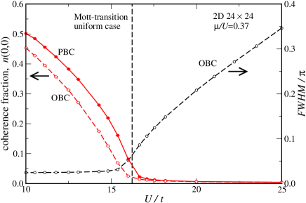
Figure 17: Evolution of the coherence fraction, i.e. the height of the coherence peak, $n(0,0)$, as a function of $U/t$ while tuning $t$ along the constant $\mu/U=0.37$ scan of Fig. 14, for bosons on a $24\times 24$ sites square lattice for both periodic (PBC) and open (OBC) boundary conditions. For OBC the full width at half maximum ($FWHM$) of the coherence peak is also shown, clearly signaling the onset of the Mott phase. The Mott transition point is indicated by the vertical dashed line.

Phase coherence is signaled by a pronounced coherence peak in the momentum distribution function, $n({\bf k}=0)$. This can be seen from Fig. 16, which shows $n({\bf k})$ for the commensurate momenta along the $k_{x}$-axis of momentum space for different values of $U/t$ for a $24\times 24$ sites system with PBC. The evolution of $n(0)$ while tuning through the transition is shown in Fig. 17. It clearly marks the loss of coherence in the Mott insulator.

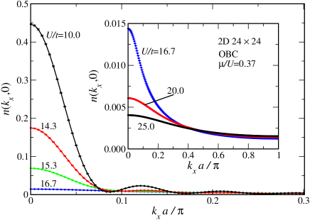
Figure 18: Momentum distribution function of bosons on a 24$\times$24-site square lattice with open boundary conditions, corresponding to an infinitely sharp trapping potential, along the line $(0,0)$-$(\pi/a,0)$ in momentum space, for different values of $U/t$, while tuning $t$ along the constant $\mu/U=0.37$ scan of Fig. 14. Within the superfluid regime satellite peaks appear, which diminish upon emergence of the Mott phase.

While for PBC a discrete set of commensurate momenta exists, for OBC states of arbitrary momenta can be occupied. In the QMC simulations, we measured the momentum distribution function on a mesh covering $10\times L$ momenta in the first Brillouin zone along the $k_{x}$-axis. The resulting momentum distribution functions for different values of $U/t$ are shown in Fig. 18. Similar to the case of PBC, the loss of coherence upon entering the Mott phase is signaled by a reduction of the coherence fraction, $n(0)$, as seen from Fig. 17. Also note the pronounced fine structures in $n({\bf k})$ for $U/t=10.0$, deep in the superfluid regime, and the complete absence of such structures for larger values of $U/t$.

Using a Ornstein-Zernike form for the coherent part for the momentum distribution function,

$$n({\bf k})=\frac{n(0)}{1+{\bf k}^{2}\xi^{2}},$$ (13)

where $\xi$ denotes the coherence length, we can obtain $\xi$ from the full width at half maximum ($FWHM$) of the coherence peak,

$$FWHM=\frac{2}{\xi}.$$ (14)

In the thermodynamic limit, the coherence length diverges in the superfluid regime. On a finite system it is bounded from above by the linear system size $L$, and decreases to zero deep inside the Mott insulating regime. We thus expect an increase of the $FWHM$, from its minimum value of $2/L$ in the superfluid regime, upon driving the system through the Mott transition. This behavior can indeed be seen in Fig. 17, which shows the $FWHM$ as a function of $U/t$ for the $24\times 24$ sites closed box. The $FWHM$ is at its lowest value of about $2/24$ left of the Mott transition, and increases due to loss of coherence beyond this point.

V.2 Parabolic traps in 2D

After our analysis of the homogeneous system, we are now in position to discuss the evolution of a confined Bose gas in a 2D optical lattice while increasing the lattice depth, i.e. decreasing the hopping, $t$. In the following, we will take the system along a path of constant chemical potential, $\mu/U=0.37$, in a parabolic trap of curvature $V/U=0.002$. An illustration of the path taken in our simulations is shown in Fig. 19.

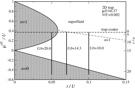
Figure 19: Variation of $\mu^{\rm eff}$ in a two dimensional parabolic trap with curvature $V/U=0.002$ for three different values of $U/t$ while tuning $t$ along a constant $\mu/U=0.37$ scan, shown within the phase diagram of the Bose Hubbard model on the square lattice. Along the dashed dotted line the density has a constant value of $n=1$.

As discussed in Sec. III, we can use a local potential approximation for a qualitative description of the inhomogeneous density profile of the trap, by employing the local value of $\mu^{\rm eff}$. For a given value of $U/t$, we can therefore represent the confined system by a vertical line in the phase diagram of the Bose Hubbard model on the square lattice. This representative vertical line is then shifted towards smaller values of $t$, during our constant $\mu$ scan. While for large values of $t$ the system will be superfluid, from Fig. 19 we expect the appearance of a central Mott plateau for smaller hopping amplitudes.

In order to determine accurately the position of the Mott plateau formation, we monitor the evolution of the density in the trap center, which is shown in Fig. 20 as a function of the inverse hopping, $U/t$.

Figure 20: Top: Radial density distribution of bosons within a two dimensional parabolic trap with curvature $V/U=0.002$ for different values of $U/t$ for $\mu/U=0.37$. Bottom: Evolution of the density in the trap center while tuning $t$ along a constant $\mu/U=0.37$ scan. For comparison the density of the uniform system along the same constant $\mu$ scan is shown. The arrow indicates the threshold for Mott plateau formation within the trap, which deviates by about 6% from the position of the Mott transition in the uniform case (vertical dashed line).

In accordance with Fig. 19, the trap center has a density larger than 1 for small values of $U/t$. Upon increasing $U/t$, the central density decreases, closely following the path of the homogeneous system. It crosses the value 1 for $U/t\approx 13.13$, as expected from Fig. 19, then undergoes a minimum, and reaches 1 for $U/t\approx 16.7$, where a Mott plateau starts to form. Apart from the critical region of the homogeneous 2D system, the density in the center of the trap closely follows the behavior in the uniform case along the same constant $\mu$ scan. The rather smooth approach towards a central density of $1$ is in agreement with the observations in Sec. IV.3 of the absence of critical fluctuations inside the trap. In addition to this qualitative difference to the homogeneous case, the local potential approximation underestimates the lower value of $U/t$ for Mott plateau formation by about 6%, as seen from Fig. 19.

Having determined the value of $U/t$ for the onset of the central Mott plateau from measurements of the density distribution, we turn to a discussion of the momentum distribution function of bosons inside the parabolic trap and its evolution upon increasing the inverse hopping, $U/t$.

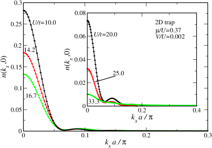
Figure 21: Momentum distribution function of bosons in a two dimensional parabolic trap with curvature $V/U=0.002$ along the line $(0,0)$-$(\pi/a,0)$ in momentum space, for different values of $U/t$ while tuning $t$ along the constant $\mu/U=0.37$ scan of Fig. 20. Satellite peaks near $(k_{x},k_{y})=(0.1\pi/a,0)$ appear unrelated to the phase structure within the trap.

In Fig. 21 the momentum distribution function $n({\bf k})$ is shown for different values of $U/t$ along the constant $\mu/U=0.37$ scan of Fig. 20. From these data it is obvious that the presence of the fine structure peak near $k_{x}a/\pi\approx 0.1$, reflecting the typical radial extent, $R\approx 20a$, of the confined Bose gas, is not related to the presence of a central Mott plateau, in agreement with earlier observations in Sec. V.

Analyzing the data further, we show in Fig. 22 the coherence fraction, $n({\bf k}=0)$, and the $FWHM$ of the coherence peak as a function of $U/t$. In marked contrast to the uniform case (Fig. 17), but in agreement with experimental findings greiner , the coherence fraction does not display distinct features upon emergence of a central Mott plateau, but instead decreases rather smoothly over a broader range than for the uniform system. This behavior is expected as it reflects the coexistence of both a Mott plateau region and a surrounding superfluid.

Similar broadenings are observed in the evolution of the $FWHM$, which becomes rather flat in the region where Mott plateau formation sets in. Since changes in the $FWHM$ are thus small near the threshold, care has to be taken when extrapolating data taken for large values of $U/t$ down to the flat region. For example, a linear extrapolation using the last two data points in Fig. 22, would overestimate the threshold for Mott plateau formation by more than 60% of its actual value.

However, we find that the $FWHM$ starts to increase well below the threshold for Mott plateau formation. Furthermore, beyond this point a change in curvature of the graph is observed, with an inflection point located at the threshold point. In fact, we found the presence of such inflection points in the $FWHM$ graphs at the transition point to be a generic feature for different trapping curvatures and dimensionalities, as will be shown below. This feature thus appears to be a reliable indication for the onset of Mott plateau formation in confined Bose systems. Although the $FWHM$ is accessible experimentally esslinger , limited resolution can make the location of the inflection point difficult, as we found the $FWHM$ graphs to be rather flat in this region.

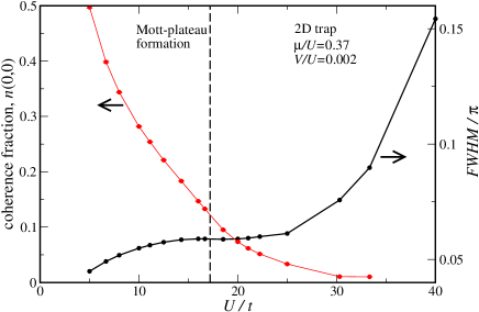
Figure 22: Evolution of the coherence fraction, i.e. the height, $n(0,0)$, and of the full width at half maximum ($FWHM$) of the coherence peak as a function of $U/t$ while tuning $t$ along the constant $\mu/U=0.37$ scan of Fig. 20 for bosons in a two dimensional parabolic trap with curvature $V/U=0.002$. The threshold for Mott plateau formation is indicated by the dashed line.

V.3 Parabolic traps in 3D

We now present results of QMC simulations of the Bose Hubbard model for bosons confined in 3D parabolic traps. Performing an analysis like in the 2D case, we find that similar generic features as those obtained in 2D apply to these 3D systems as well.

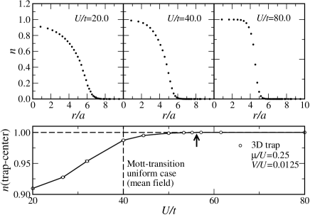
Figure 23: Top: Radial density distribution of bosons within a three dimensional parabolic trap with curvature $V/U=0.0125$ for different values of $U/t$ for $\mu/U=0.25$. Bottom: Evolution of the density in the trap center while tuning $t$ along a constant $\mu/U=0.25$ scan. The arrow indicates the threshold for Mott plateau formation within the trap, which deviates by about 30% from the position of the Mott transition in the uniform case within mean field theory (vertical dashed line).

In particular, we consider a parabolic trap with curvature $V/U=0.0125$, and study the system’s states for different values of $t/U$ along a line of constant $\mu/U=0.25$. For a value of $U/t=20$, the system is still deep in the superfluid regime, as seen in Fig. 23, reflecting the increased strength of the kinetic energy, due to the larger dimensionality. Upon decreasing the hopping $t$, a Mott plateau forms in the trap center. In Fig. 23 we trace the boson density in the trap center as a function of $U/t$, in order to locate the threshold for emergence of the Mott plateau region, indicated by the vertical arrow. Similar to the 2D case, the central density approaches the value of 1 with a flat slope. Within mean field theory fisher ; monien and the local potential approximation, the threshold would be underestimated by about 30%, as indicated by the dashed vertical line in Fig. 23.

Analyzing the momentum distribution functions shown in Fig. 24, we observe similar behavior as in the 2D system: (i) As seen from Fig. 25, at the threshold for Mott plateau formation, the coherence fraction is still about 10% of the overall bosonic density and decreases over a rather broad range of parameters.

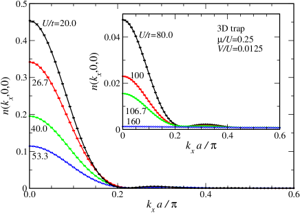
Figure 24: Momentum distribution function of bosons in a three dimensional parabolic trap with curvature $V/U=0.0125$ along the line $(0,0,0)$-$(\pi/a,0,0)$ in momentum space, for different values of $U/t$ while tuning $t$ along the constant $\mu/U=0.25$ scan of Fig. 23. Satellite peaks near ${\bf k}=(0.3\pi/a,0,0)$ appear unrelated to the phase structure within the trap.

(ii) The $FWHM$ of the coherence peak undergoes a change of curvature with an inflection point being located at the threshold for Mott plateau formation. The presence of this inflection point thus provides a robust indication of density restructurings also inside 3D traps. (iii) As in 2D, we find the presence of satellite peaks to be unrelated to the local density structure, as seen from Fig. 24. (iv) The position of the fine structure peak is indicative of the spatial extent of the bosonic cloud. In fact, the broad peak observed at $k_{x}\approx 0.3\pi/a$ in Fig. 24 corresponds well to the radial extent $R\approx 6a$ of the Bose gas.

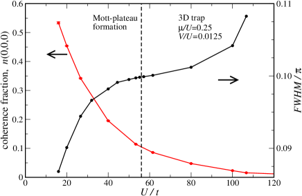
Figure 25: Evolution of the coherence fraction, i.e. the height, $n(0,0,0)$ and of the full width at half maximum ($FWHM$) of the coherence peak as a function of $U/t$ while tuning $t$ along the constant $\mu/U=0.25$ scan of Fig. 23 for bosons in a three dimensional parabolic trap with curvature $V/U=0.0125$. The threshold for Mott plateau formation is indicated by the dashed line.

V.4 Parabolic traps in 1D

Finally, we extend our analysis to the case of a 1D parabolic trap. Fixing the chemical potential to a value of $\mu/U=0.37$, similar to the 2D case, we study the system for different values of the hopping amplitude, $t$. In the upper part of Fig. 26 the spatial density distribution is shown for three different values of $U/t$. The evolution of the density in the trap center as a function of $U/t$ is shown in the lower part of Fig. 26.

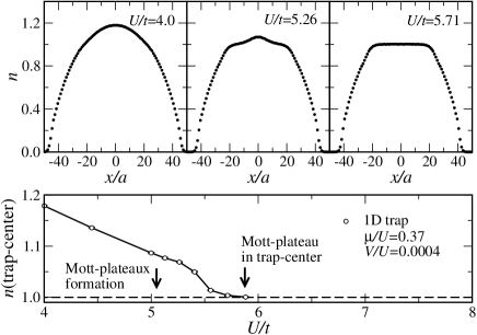
Figure 26: Top: Spatial density distribution of bosons within a one dimensional parabolic trap with curvature $V/U=0.0004$ for different values of $U/t$, for $\mu/U=0.37$. Bottom: Evolution of the density in the trap center while tuning $t$ along a constant $\mu/U=0.37$ scan. The threshold for Mott plateaux formation within the trap, and merging of the two plateaux are indicated by vertical arrows.

For $U/t=4.0$ the system is in the fully superfluid regime, with no Mott plateaux present. Upon increasing $U/t$, there appears a finite regime, where two Mott plateaux emerge well outside the center of the trap. These plateaux eventually merge into an extended Mott plateau at a larger value of $U/t$. The position of these points is marked by the arrows in the lower part of Fig. 26. This emergence of an intermediate regime with two well separated Mott plateaux is expected from the shape of the first Mott lobe in 1D kuehner , and the chosen value of $\mu/U=0.37$, and follows using a local potential approximation, similar to the case of the 2D trap considered above. The reason why such an intermediate regime is observed in our 1D simulations, but not for the 2D case, is that in 1D the largest extent of the first Mott lobe has a critical value of $\mu/U\approx 0.10$ which is below our chosen value of $\mu/U=0.37$, whereas the critical value of $\mu/U=0.42$ in 2D is above that value.

The corresponding momentum distribution functions are shown in Fig. 27. Compared to the higher dimensional cases, the momentum distribution functions appear broad, indicating larger incoherent contributions. This is expected, as in 1D long range coherence cannot develop, even at zero temperature. Similar to the higher dimensional cases, we observe broad fine structure peaks in $n(k)$, restricted however to $U/t$ below the threshold for Mott plateau formation. At larger values of $U/t$, such fine structure is not resolved due to the large incoherent contribution.

Analyzing the momentum distribution functions as shown in Fig. 28, we find that the graph of $FWHM$ as a function of $U/t$ exhibits two characteristic features: The increase of the slope for $U/t$ near $5.0$ corresponds well to the threshold for the formation of the two Mott plateaux. The growth of the two Mott plateaux regions results in the fast decrease of the coherence length in this regime. Beyond $U/t\approx 5.7$, the increase in the $FWHM$ is reduced, indicating that the two plateaux have merged into a single plateau, which now grows at only two ends. The $U/t$ dependence of the coherence fraction $n(0)$ also indicates the merging of the two Mott plateaux, by a reduced decrease in $U/t$ beyond $U/t\approx 5.7$.

Recently Kollath et al. kollath studied the 1D case using the Density Matrix Renormalization Group method. Their results are in perfect agreement with our observations.

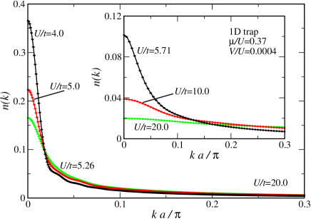
Figure 27: Momentum distribution function of bosons in a one dimensional parabolic trap with curvature $V/U=0.0004$ along the line $0$-$\pi/a$ in momentum space, for different values of $U/t$ while tuning $t$ along the constant $\mu/U=0.37$ scan of Fig. 26.

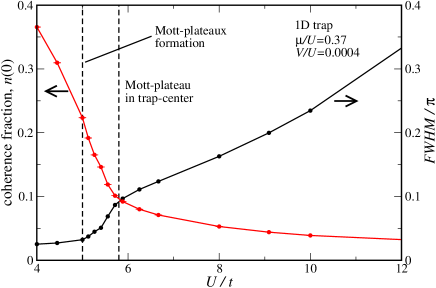
Figure 28: Evolution of the coherence fraction, i.e. the height, $n(0)$, and of the full width at half maximum ($FWHM$) of the coherence peak as a function of $U/t$ while tuning $t$ along the constant $\mu/U=0.37$ scan of Fig. 26 for bosons in a one dimensional parabolic trap with curvature $V/U=0.0004$. The threshold for Mott plateaux formation within the trap, and for the collapse of the two plateaux into a single plateau are indicated by dashed lines.

VI Discussion and conclusion

Our quantum Monte Carlo simulations provide insight into the physics of trapped bosonic systems on lattices. The validity of a local potential approximation, where local quantities such as the local density or compressibility depend mainly on the value of the local chemical potential, is confirmed by an excellent data collapse of local quantities on single curves. This single curve is however not the same as for the homogeneous bulk system; the differences are particularly pronounced in the interesting vicinity of the transition layer between Mott insulators and superfluid in the parabolic trap. There the singularities due to quantum critical behavior are removed and replaced by smooth and broad features.

While the behavior of the homogeneous system can give a qualitative overview of the phase structure realized locally inside the parabolic trap, quantitative results can only be obtained by numerical (quantum Monte Carlo) simulations of realistic systems. Results for realistic 2D parabolic traps of a size comparable to experiments have been presented here, as well as an analysis of the 1D situation. Three dimensional simulations have so far been performed only on systems with linear dimensions 2-3 times smaller than experimental realizations, but realistic simulations will be possible in the near future using faster computers and improved algorithms.

An effective ladder model, which quantitatively models the realistic trapped system, provides clear evidence for the absence of quantum critical behavior in parabolic confinement potentials. The ladder model allows us to exclude the randomness imposed on the superfluid ring by the underlying square lattice structure as the source of this absence of quantum criticality. Instead, the divergences due to quantum critical fluctuations are suppressed by the inhomogeneity, and the coupling to the rest of the system. It will be very interesting to develop an effective action for this coupling, which might explain the power law behavior observed in Ref. muramatsu ; bergkvist . Furthermore, the observed absence of quantum criticality in both parabolic traps and ladder models with a gradient in the chemical potential connecting different Mott plateau regions calls for future investigations, and extension to fermionic models.

The absence of quantum critical behavior of bosons in parabolic confinement potentials also agrees well with the fast dynamics of the “phase transition” and the observed absence of “critical slowing down” of the dynamics in experiments greiner . Critical slowing down at a second order phase transition is caused by the long time scales taken to establish a uniform order parameter across the whole system. Small ordered domains, with differently broken $U(1)$ symmetry are quickly formed, but as these domains grow and merge, the dynamics to establish the same $U(1)$ symmetry breaking across neighboring domains slows down as the domains grow in size. The dynamics of the “quantum phase transition” in the trapped system is different: driving the system from the superfluid to the Mott insulator happens by nucleating a small Mott domain inside the trap, which then grows as the depth of the optical lattice is increased. As the Mott phase grows in volume and the superfluid phase shrinks the “quantum phase transition” is observed. This is however better viewed as a crossover with changing volume fractions of the two phases than as a phase transition: the large Mott plateau is always surrounded by a shell of coherent superfluid. Sweeping back to the superfluid phase by decreasing the depth of the optical lattice, the Mott insulator melts and atoms join the superfluid. The dynamics here is not that of two large domains merging, but that of a single atom joining the coherent superfluid and there is no critical slowing down involved in this process. It might be possible to experimentally observe critical slowing down in a trap by first driving the system deep into the Mott insulating region, then kicking it to destroy the phase coherence in the remaining superfluid shell and afterwards quickly driving it back into the superfluid.

Finally, we analyzed the behavior of the momentum distribution function, which is accessible experimentally from the interference patterns of absorption images taken after free expansion of the atomic gas. We find that the full width at half maximum of the coherence peak in the momentum distribution function, due to its relation to the coherence length in the system, yields valuable information about density restructurings inside the trap. In particular, we found an inflection point in its graph upon increasing the lattice depth well at the threshold for central Mott plateau formation. Since the graph becomes flat in this region, detection of such features requires high resolution data taken in the crossover regime.

In contrast, we found that for flat confinement potentials, realizing closed box systems, both the full width at half maximum, as well as the coherence fraction provide clear signals for the Mott transition. Furthermore, in flat trapping geometries, quantum critical fluctuations are significantly more pronouned, and allow the observation of quantum critical behavior already on optical lattices of currently available sizes. We thus expect the possible realization of flat confinement potentials zoller_privat to significantly ease the detection of true quantum criticality and the interpretation of the experimental data.

Performing quantum Monte Carlo studies for realistic systems will be important for interpreting current and future experiments on confined Bose gases in optical lattices, and for testing our quantitative understanding of these systems. Such understanding will be important, once analog quantum computers build from fermionic atoms are available, for which large scale quantum Monte Carlo simulations will not be possible.

References

- (1) M. Greiner et al., Nature 415, 39 (2002).
- (2) T. Stöferle et al., Phys. Rev. Lett. 92, 130403 (2004).
- (3) D. Jaksch et al., Phys. Rev. Lett. 81, 3108 (1998).
- (4) W. Hofstetter et al., Phys. Rev. Lett. 89, 220407 (2002).
- (5) G. G. Batrouni et al., Phys. Rev. Lett. 89, 117203 (2002).
- (6) V. A. Kashurnikov, N. V. Prokof’ev, and B. V. Svistunov, Phys. Rev. A 66 031601(R) (2002).
- (7) S. Wessel, F. Alet, M. Troyer, and G. G. Batrouni, to appear in Adv. Solid State Phys. (2004).
- (8) A.W. Sandvik and J. Kurkijärvi, Phys. Rev. B 43, 5950 (1991); A. W. Sandvik, J. Phys. A 25, 3667 (1992).
- (9) A.W. Sandvik, Phys. Rev. B 59, R14157 (1999).
- (10) O. F. Syljuåsen and A. W. Sandvik, Phys. Rev. E 66, 046701 (2002).
- (11) O. F. Syljuåsen, Phys. Rev. E 67, 046701 (2003).
- (12) F. Alet, S. Wessel, and M. Troyer, Report cond-mat/0308495.
- (13) R. Roth and K. Burnett, Phys. Rev. A 67, 031602(R) (2003).
- (14) L. Pollet, S. Rombouts, and K. Heyde, J. Dukelsky Phys. Rev. A 69, 043601 (2004).
- (15) C. Schroll, F. Marquardt, and C. Bruder, Report cond-mat/0404576.
- (16) C. Kollath et al., Phys. Rev. A 69, 031601(R) (2004).
- (17) S. Bergkvist, P. Henelius, and A. Rosengren, Report cond-mat/0404395.
- (18) M. Rigol and A. Muramatsu, Report cond-mat/0403078.
- (19) J. Oliva, Phys. Rev. B 39, 4197 (1989).
- (20) K. Damle et al., Europhys. Lett. 36, 7 (1996).
- (21) M. Rigol et al., Phys. Rev. Lett. 91, 130403 (2003).
- (22) G. G. Batrouni, R. T. Scalettar, and G. T. Zimanyi, Phys. Rev. Lett. 65, 1765 (1990).
- (23) M. P. A. Fisher et al., Phys. Rev. B 40, 546 (1989).
- (24) J. K. Freericks and H. Monien, Europhys. Lett. 26, 545 (1994).
- (25) J. K. Freericks and H. Monien, Phys. Rev. B 53, 2691 (1996).
- (26) E. L. Pollock and D. M. Ceperley, Phys. Rev. B 36, 8343 (1987); A. W. Sandvik, Phys. Rev. B 56, 11678 (1997).
- (27) F. Alet and E. S. Sørensen, Report cond-mat/0401236.
- (28) T. D. Kühner, S. R. White, and H. Monien, Phys. Rev. B 61, 12474-12489 (2000).
- (29) P. Zoller, private communications.
-
(30)
M. Troyer et al., Lecture Notes in Computer
Science 1505, 191 (1998). Source codes of the libraries can
be obtained from
http://alps.comp-phys.org/.