Phase diagrams of a classical two-dimensional Heisenberg antiferromagnet with single-ion anisotropy

Abstract

A classical variant of the two-dimensional anisotropic Heisenberg model reproducing inelastic neutron scattering experiments on La₅Ca₉Cu₂₄O₄₁ [M. Matsuda et al., Phys. Rev. B 68, 060406(R) (2003)] is analysed using mostly Monte Carlo techniques. Phase diagrams with external fields parallel and perpendicular to the easy axis of the anisotropic interactions are determined, including antiferromagnetic and spin-flop phases. Mobile spinless defects, or holes, are found to form stripes which bunch, debunch and break up at a phase transition. A parallel field can lead to a spin-flop phase.

I Introduction

The compounds (La,Ca)₁₄Cu₂₄O₄₁ have been studied experimentally rather extensively in recent years.ca ; m1 ; miz ; m2 ; am ; ka ; windt ; rk ; m4 They display interesting low-dimensional magnetic properties arising from Cu₂O₃ two-leg ladders and CuO₂ chains. In addition, for La_14-xCa_xCu₂₄O₄₁ there is an intriguing interplay between spin and charge ordering due to hole doping when $x>8$.

In particular, La₅Ca₉Cu₂₄O₄₁ exhibits, at low temperatures and small fields, antiferromagnetic long range order associated with the CuO₂ chains which are oriented along the $c$ axis. The Cu²⁺ ions in those chains carry a spin-1/2. The spins are ordered ferromagnetically in the chains, while the interchain coupling in the $ac$–planes is antiferromagnetic. The magnetic interactions between the $ac$–planes are believed to be very weak. The couplings in the $ac$–planes are anisotropic with an easy axis along the $b$ axis, i.e. the magnet has an Ising-like character.am ; ka ; rk ; m4 Holes may originate from the La and Ca ions, transforming Cu ions into spinless quantities, with a hole content of about 10 percent.nu

Experiments on La₅Ca₉Cu₂₄O₄₁ include thermodynamic measurements on the specific heat, magnetization, and susceptibility am ; rk as well as electron spin resonance ka and neutron scattering.miz ; rk Motivated by the experimental findings, different models have been proposed and studied. Firstly, a two-dimensional Ising model has been introduced,spbk ; hs where the spins correspond to the Cu²⁺ ions, and mobile spinless defects mimic the holes. In addition to the ferromagnetic intrachain and antiferromagnetic interchain couplings between neighboring spins, a rather strong and antiferromagnetic exchange between next-nearest chain spins separated by a hole is assumed. The model has been shown to describe, at low temperatures, antiferromagnetic domains separated by quite straight defect lines which break up at a phase transition where also the long range magnetic order gets destroyed. The stripe instability is caused by an effectively attractive interaction between the defects mediated by the antiferromagnetic interchain couplings.

Even more recently, a two-dimensional anisotropic Heisenberg model has been shown by Matsuda et al. to reproduce the measured spin-wave dispersions which supposedly result from the collective spin excitations of the Cu²⁺ ions in the $ac$–planes.m4 Our subsequent Monte Carlo simulations on the classical variant of the model seem to indicate, however, that some of its thermodynamic properties tend to deviate from experimental findings.ls In particular, in an external field along the $b$ axis, at low temperatures, the field dependence of the susceptibility of the anisotropic Heisenberg model disagrees with the measured behavior. The disagreement can probably not be resolved by invoking quantum effects. In particular, the critical temperature of the model seems to be significantly lower than the measured one, as can be seen by comparing results on related quantum and classical models.ls ; cuc ; se Indeed, in this paper we will show that the qualitative properties of the phase diagram of the model are not affected qualitatively by quantum effects.

In any event, the classical variant of the model of Matsuda et al. deserves to be studied in more detail. Apart from the previous qualitative comparison ls with experimental data, the classical model is of genuine theoretical interest as well. Perhaps most interestingly, the phase diagram in the (temperature,field)–plane is worth studying in the context of two-dimensional anisotropic Heisenberg models. Due to the anisotropy, there is a spin-flop phase when applying a sufficiently high external field along the $b$ axis. In two dimensions, that phase has interesting properties as it is believed to be of Kosterlitz-Thouless type with spin correlations decaying algebraically with distance. Furthermore, the boundary line of the antiferromagnetic phase as well as the transition between the antiferromagnetic and the spin-flop phase has been discussed controversially for anisotropic nearest-neighbor Heisenberg models. In three and higher dimensions, there is a bicritical point where the antiferromagnetic, the spin-flop, and the paramagnetic phases meet.fn As it is well known, such a point could occur in two dimensions only at zero temperature (Mermin-Wagner theorem). Actually, different scenarios have been proposed.bl However, simulations and other analyses on classical models lead to controversial results.bl ; cp Fairly recently, a $S=1/2$ quantum version has been simulated suggesting a topology of the phase diagram with a tricritical and a critical end point.sch Our work will deal with this aspect. Note that quasi two-dimensional anisotropic Heisenberg antiferromagnets exhibiting a spin-flop phase have attracted much experimental attention already some years ago.jon ; rau ; stei Well-known examples are Rb₂MnCl₄ and K₂MnF₄. The approach of our study may be also useful for the correct theoretical analysis of models describing these materials.

Our main emphasis will be on a classical variant of the model by Matsuda et al. obtained from the spin-wave dispersions of La₅Ca₉Cu₂₄O₄₁. In addition, in an attempt to include possible effects due to the holes, we shall extend the model by allowing for mobile defects following the previous considerations.spbk In fact, the defects again form stripes which are destabilized at a phase transition. Bunching and debunching of the stripes are novel features. Effects of an external field along the $b$ axis will also be considered.

The layout of the article is as follows: In the next section, the model will be introduced. Its phase diagrams, without defects and applying external fields parallel and perpendicular to the easy axis of the magnetic interactions, will be presented in Sec. III. The possible influence of defects on thermal properties will be discussed in section IV, followed by a summary.

II The model, simulations, and quantities of interest

Following Matsuda et al.,m4 the magnetic properties of La₅Ca₉Cu₂₄O₄₁ depend on the $\text{Cu}^{2+}$ ions located in the $ac$–planes, having a centered rectangular geometry as depicted in Fig. 1. Based on their spin-wave analysis, the spins ($S=1/2$) of the ions couple along the CuO₂ chains, i.e. along the $c$ axis, through nearest neighbor, $J_{c1}$, and next-nearest neighbor, $J_{c2}$, exchange constants, with $J_{c1}=-0.2$ meV being antiferromagnetic and $J_{c2}=0.18$ meV being ferromagnetic. The ferromagnetic ordering in the chains is due to the strong antiferromagnetic interchain couplings, see also Fig. 1: $J_{ac1}=-0.681$ meV refers to the two nearest neighbors in the adjacent chain, and $J_{ac2}=0.5J_{ac1}=-0.3405$ meV denotes the couplings to the two next-nearest neighbors.

Importantly, there is an uniaxial exchange anisotropy favoring alignment of the spins along the $b$ axis. Its contribution to the different couplings cannot be determined in the spin-wave analysis, and only its integral effect on the gap in the dispersion is quantified.m4 When going over to a classical description with spins of fixed length, say, one, the total anisotropy may be mimicked by a single-ion term. Such a term would be, of course, merely a trivial constant and unphysical for a quantum system with $S$= 1/2. The single-ion term, avoiding ambiguities in distributing the anisotropy among the different couplings, is quite reasonable in the classical variant. It leads to about the same transition temperature without field as various exchange anisotropies of the same overall magnitude.ls In addition, the entire phase diagram seems to be not affected by the type of anisotropy. The anisotropy has been estimated from the gap energy to be $D=-0.211$ meV.m4 Thence the Hamiltonian can be written as m4 ; ls

$${\cal H} = -J_{c1}\sum\limits_{(l,m)}\mathbf{S}_{l,m}\mathbf{S}_{l+1,m}-J_{c2}\sum\limits_{(l,m)}\mathbf{S}_{l,m}\mathbf{S}_{l+2,m}-J_{ac1}\sum\limits_{(l,m)}\mathbf{S}_{l,m}(\mathbf{S}_{l,m+1}+\mathbf{S}_{l+1,m+1})$$

$${}-J_{ac2}\sum\limits_{(l,m)}\mathbf{S}_{l,m}(\mathbf{S}_{l-1,m+1}+\mathbf{S}_{l+2,m+1})+D\sum\limits_{(l,m)}(S_{l,m}^{z})^{2}-H_{\alpha}\sum\limits_{(l,m)}S_{l,m}^{\alpha},$$ (1)

where $\mathbf{S}_{l,m}=(S_{l,m}^{x},S_{l,m}^{y},S_{l.m}^{z})$ denotes the spin at the $l$–th site in the $m$–th chain; $\alpha$ refers to differently oriented magnetic fields, with $\alpha=z$ for the field parallel to the easy axis, and $\alpha=x$ or $y$ for a field perpendicular to it, i.e. along the $a$ or $c$ axis.

Figure 1: Sketch of the the magnetic interactions for the two-dimensional anisotropic Heisenberg model of Matsuda et al.m4 The dots denote the sites of the Cu²⁺ ions in the $ac$–plane of La₅Ca₉Cu₂₄O₄₁.

Extending this Hamiltonian of Matsuda et al., we introduce defects $S_{l,m}=0$, induced by the holes originating from the La and Ca ions.spbk We neglect direct interactions between the defects, and there are no couplings between a defect and a spin. Next-nearest neighbor spins in the same chain, $S_{l,m}$ and $S_{l\pm 2,m}$, with a defect in between them are coupled by the exchange constant $J_{0}$ (replacing $J_{c2}$), which we presume to be antiferromagnetic and rather strong as before, i.e. of several meV.spbk Specifically, we choose $J_{0}=-6.25$ meV. Thence, the Hamiltonian (1) is augmented by the term

$${\cal H}_{d}=-J_{0}\sum\limits_{(l,m)}S_{l,m}S_{l+2,m}(1-n_{l+1,m}),$$ (2)

with $n_{l,m}=0,1$ being the occupation variable of a spin at site $(l,m)$. The defects are allowed to hop to a neighboring site in a chain, transforming the spin at that site into a defect and leaving a new spin with arbitrary orientation at its initial site. The probability of such a process is determined by the Boltzmann factor of the change in the magnetic energy, Eqs. (1) and (2), associated with the hop.spbk It is easily incorporated in Monte Carlo simulations.

As before,spbk we assume that defects are separated along the chain by at least one spin. The number of defects in each chain will be taken to be 10 percent of the number of sites in that chain. The defect concentration is then close to that in La₅Ca₉Cu₂₄O₄₁.nu ; rk

We shall study the model, with and without defects, using, apart from ground state calculations, standard Monte Carlo techniques with local elementary processes changing at randomly chosen sites the spin orientation and moving defects to neighboring sites. In the simulations, we consider lattices with the same number $L$ of chains and of sites per chain, i.e. with a total of $L^{2}$ sites. Full periodic boundary conditions are employed. To study finite-size effects allowing extrapolations to the thermodynamic limit, $L\longrightarrow\infty$, we consider typically sizes ranging from $L$=10 to $L$=200. Each run consists of at least $10^{6}$ and up to $5\times 10^{6}$ Monte Carlo steps per site. To obtain averages and error bars, we take into account the results of up to 10 realizations using different random numbers.

We compute both quantities of direct experimental interest as well as other quantities which enable us to determine critical properties and the phase transition lines. In particular, we recorded the specific heat $C$, both from the fluctuations and from the temperature derivative of the energy per site $E$. In the absence of defects, various magnetizations were computed. Especially, we recorded

(i) the $\alpha$–component of the magnetization to study the response to a field in the $\alpha$ direction, with $\alpha=x,y,z$,

$$<M^{\alpha}>=<\sum\limits_{(l,m)}S_{l,m}^{\alpha}>/L^{2};$$ (3)

(ii) the $z$–component of the absolute value of the staggered magnetization $M_{s}^{z}$ and the square of the staggered magnetization to describe the order in the antiferromagnetic phase,

$$<|M_{s}^{z}|>=<|\sum\limits_{(\mathrm{all}\,l,\,m\,\mathrm{even})}S_{l,m}^{z}-\sum\limits_{(\mathrm{all}\,l,\,m\,\mathrm{odd})}S_{l,m}^{z}|>/L^{2},$$ (4)

(summing separately over sites in even and odd chains), and similarly for $<(M_{s}^{z})^{2}>$; and

(iii) the square of the transverse sublattice magnetization to describe the Kosterlitz-Thouless character of the spin-flop phase when applying a field along the easy axis,

$$<M_{xy}^{2}>=<\sum\limits_{\alpha=x,y}\Big{[}\Big{(}\sum\limits_{(\mathrm{all}\,l,\,m\,\mathrm{even})}S_{l,m}^{\alpha}\Big{)}^{2}+\Big{(}\sum\limits_{(\mathrm{all}\,l,\,m\,\mathrm{odd})}S_{l,m}^{\alpha}\Big{)}^{2}\Big{]}>\big{/}(L^{4}/2).$$ (5)

In addition, we recorded the magnetic susceptibilities $\chi^{\alpha}$, which may be computed from the fluctuations or field derivatives of the corresponding magnetizations, $<M^{\alpha}>$, and the (finite lattice) staggered susceptibility $\chi_{s}^{z}$ defined by

$$\chi_{s}^{z}=L^{2}\,\big{(}<(M_{s}^{z})^{2}>-<|M_{s}^{z}|>^{2}\big{)}/2.$$ (6)

To identify the type of transition from the antiferromagnetic to the paramagnetic and the spin-flop phases, the fourth-order, size dependent cumulant of the staggered magnetization, the Binder cumulant bin $U_{L}$, is rather useful:

$$U_{L}=1-<(M_{s}^{z})^{4}>/\big{(}3<(M_{s}^{z})^{2}>^{2}\big{)},$$ (7)

where $<(M_{s}^{z})^{4}>$ is defined in analogy to $<(M_{s}^{z})^{2}>$.

In the presence of defects we studied, apart from the specific heat, magnetization and susceptibility, also microscopic quantities describing the topology and stability of the defect stripes,spbk ; hs including the average minimal distance between defects in adjacent chains and the density of defect pairs. Results will be discussed in Sec. IV.

III Phase diagrams in the absence of defects

We analysed the anisotropic Heisenberg model of Matsuda et al.m4 applying external fields along the easy axis ($H_{z}$) and perpendicular to it (say, $H_{x}$), and varying the temperature, see the Hamiltonian (1). The resulting phase diagrams are depicted in Fig. 2.

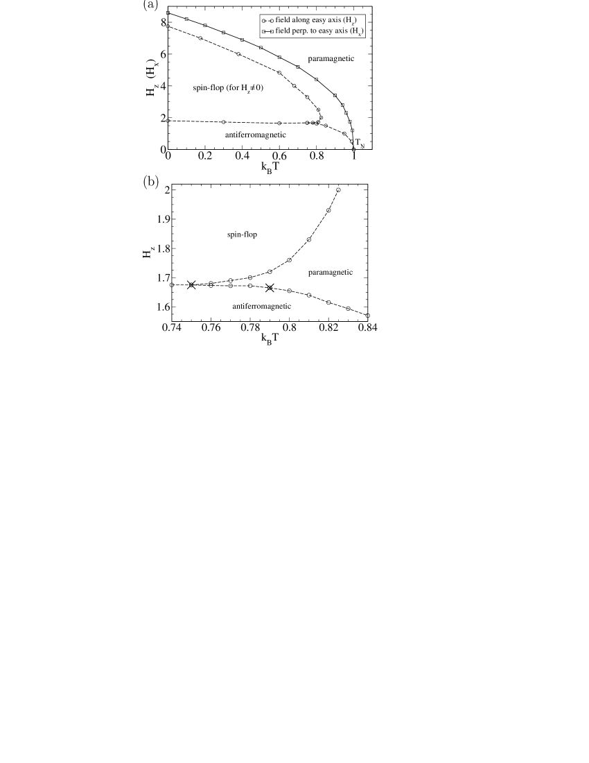
Figure 2: Phase diagram of the model without defects, with fields parallel, $H_{z}$, and perpendicular, $H_{x}$, to the easy axis. (a) Global phase diagram, (b) details in the ($T,H_{z}$) plane. Crosses denote approximate locations of the tricritical point and the critical end point (see text).

In the case of a field $H_{x}>0$ perpendicular to the easy axis one encounters, at zero temperature and small fields, $H_{x}<H_{x}^{\mathrm{pm}}$, an antiferromagnetic ground state with the non-zero, field-dependent $z$–component of the spins in each chain pointing in the same direction and alternating sign from chain to chain, $S_{l,m}^{z}=-S_{l,m+1}^{z}$. At zero temperature and larger fields, $H_{x}>H_{x}^{\mathrm{pm}}$, the magnetic field term dominates, and the spins are aligned along the direction of the field, $S_{l,m}^{x}$=1. The critical field $H_{x}^{\mathrm{pm}}$ is readily calculated. Inserting the values of the intrachain, $J_{c1}$ and $J_{c2}$, and interchain coupling constants, $J_{ac1}$ and $J_{ac2}$, as well as the spin anisotropy, $D$, as stated in the preceeding section, one gets $H_{x}^{\mathrm{pm}}=8.594..$ meV. Certainly, this is an artificial unit, which had to be transcribed into the standard unit Tesla, taking into account the $g$-factor and the actual spin value, when comparing results for non-vanishing fields quantitatively to experimental findings. However, in the context of our analysis the artificial unit will be sufficient. In the following, the unit ”meV” will be suppressed in all expressions for the energy, $k_{B}$ times temperature ($k_{B}T$), and the magnetic field.

At non-zero temperatures, a critical line arises from $(T=0,H_{x}=H_{x}^{\mathrm{pm}})$ ending at $(T=T_{N},H_{x}=0)$, see Fig. 2a. The transition separates the ordered antiferromagnetic phase with a non-zero staggered magnetization $<|M_{s}^{z}|>$, see Eq. (4), from the disordered (paramagnetic) phase, where $<|M_{s}^{z}|>=0$. The phase transition is expected to be continuous and of Ising type, i.e. with the well-known critical exponents of the two-dimensional Ising model. The critical line has been obtained by fixing either the temperature and varying the field or by fixing the field and varying the temperature. Then standard finite-size analyses on the peak positions of the specific heat, $T_{m}^{C}(L)$, were done. Indeed, these positions approach, for sufficiently large system sizes, the critical temperature $T_{c}$ of the infinite system like $T_{c}-T_{m}^{C}(L)\propto 1/L$, which is consistent with the transition belonging to the Ising universality class. For illustrative purposes, some raw data on the specific heat are shown in Fig. 3.

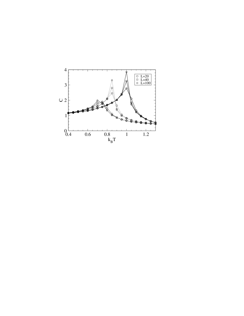
Figure 3: Specific heat vs. temperature at fixed fields $H_{x}=H_{z}=0$ (solid lines), $H_{x}=4.0$ (dotted lines), and $H_{z}=4.0$ (dashed lines), for systems, without defects, of various sizes $L$.

The thermal behavior of the staggered magnetization is shown, for a few selected examples, in Fig. 4.

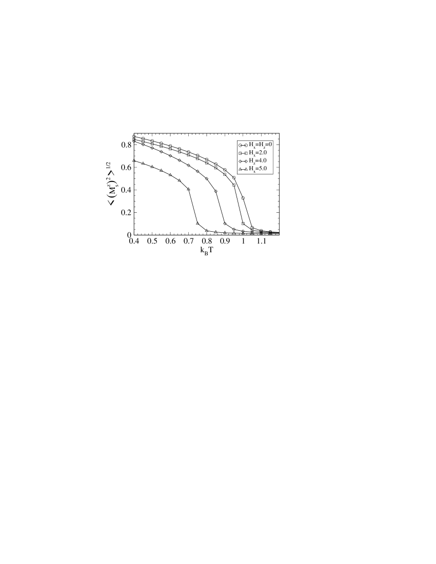
Figure 4: Staggered magnetization vs. temperature for various fields parallel ($H_{z}$) and perpendicular ($H_{x}$) to the easy axis, simulating systems, without defects, of size $L=100$.

In the case of an external field $H_{z}>0$ along the easy axis one obtains a more complex and more interesting phase diagram, see Fig. 2. In the ground state ($T=0$), one has to distinguish two critical fields, $H_{z}^{\mathrm{sf}}$ and $H_{z}^{\mathrm{pm}}$. For $H_{z}<H_{z}^{\mathrm{sf}}$, the antiferromagnetic structure, as described above, has the lowest energy. At larger fields, $H_{z}^{\mathrm{sf}}<H_{z}<H_{z}^{\mathrm{pm}}$, the spin-flop state is stable. There the $z$–component of the spins in all chains acquires the same, field-dependent value $S^{z}(H_{z})>0$. The planar, $xy$–components of the spins are aligned parallel to each other in each chain, pointing in an arbitrary direction due to the rotational invariance of the interactions in the $xy$–plane, see Eq. (1). The $xy$–components of spins in neighboring chains point in the opposite direction because of the antiferromagnetic interchain couplings. At $H>H_{z}^{\mathrm{pm}}$, one has a ferromagnetic ordering with $S^{z}=1$.

For the set of couplings obtained from the spin-wave analysis, the critical fields are $H_{z}^{\mathrm{sf}}=1.808..$ and $H_{z}^{\mathrm{pm}}=7.75$. At $H_{z}=H_{z}^{\mathrm{sf}}$, the $z$–component takes the value $S^{z}(H_{z}^{\mathrm{sf}})=0.233..$, corresponding to an angle of $76.5..$ degrees formed by the $z$ axis and the orientation of the spins.

The complete phase diagram in the $(T,H_{z})$ plane consists of the antiferromagnetic, the spin-flop and the paramagnetic or disordered states, see Figs. 2a and 2b. The antiferromagnetic phase exhibits long-range order with the staggered magnetization $M_{s}^{z}$ as order parameter. The spin-flop phase has been argued to be of Kosterlitz-Thouless character,fn ; bl ; cp ; sch where transverse spin correlations, i.e. $<S_{lm}^{x}S_{l^{\prime}m^{\prime}}^{x}+S_{lm}^{y}S_{l^{\prime}m^{\prime}}^{y}>$, decay algebraically with distance $\sqrt{(l-l^{\prime})^{2}+(m-m^{\prime})^{2}}$. Accordingly, the transverse sublattice magnetization, see Eq. (5), being the order parameter of the spin-flop phase in three dimensions, is expected to behave for $T>0$ and sufficiently large systems as

$$<M_{xy}^{2}>\propto L^{-g}$$ (8)

with $g$ approaching 1/4 at the transition from the spin-flop to the paramagnetic phase,kt and $g=2$ in the paramagnetic phase. Thence, the order parameter vanishes in the Kosterlitz-Thouless phase as $L\longrightarrow\infty$ at all temperatures $T>0$. Of course, in the disordered phase spin correlations decay exponentially with distance.

While the existence of these phases for weakly anisotropic Heisenberg antiferromagnets in two dimensions is undisputed, basic aspects of the topology of the phase diagram and especially the transitions between the antiferromagnetic phase and the spin-flop as well as the paramagnetic phases have been discussed controversially,bl ; cp ; sch and they may, indeed, depend on details of the model.

We determined the boundary line of the antiferromagnetic phase by monitoring especially the specific heat $C$, the (square of the) staggered magnetization, $<|M_{s}^{z}|>$ and $<(M_{s}^{z})^{2}>$, the staggered susceptibility, $\chi_{s}^{z}$, and the Binder cumulant, $U_{L}$, Eq. (7). A few raw data for the specific heat and the staggered magnetization are included in Figs. 3 and 4.

The transition from the antiferromagnetic to the disordered phase at low fields and high temperatures is continuous and of Ising type. Its location, as displayed in Figs. 2a and 2b, follows from finite-size analyses of the various physical quantities. The data are consistent with a logarithmic divergence of the specific heat as well as with the well-known Ising values for the critical exponents of the order parameter, $\beta=1/8$, and of the staggered susceptibility, $\gamma=7/4$.

More interestingly, the transition from the antiferromagnetic to the paramagnetic phase eventually becomes first order when increasing the field and lowering the transition temperature, with a tricritical point at $k_{B}T_{\mathrm{tr}}=0.79\pm 0.015$ and $H_{z}^{\mathrm{tr}}=1.665\pm 0.01$. The boundary line of the antiferromagnetic phase remains to be first order at lower temperatures when separating the antiferromagnetic and the spin-flop phase. The Kosterlitz-Thouless line separating the spin-flop phase from the paramagnetic (disordered) state hits the boundary of the antiferromagnetic phase in a critical end point at $k_{B}T_{\mathrm{cep}}=0.75\pm 0.015$ and $H_{z}^{\mathrm{cep}}=1.675\pm 0.01$, see Fig. 2b. Note that the phase diagram has qualitatively the same topology as the one suggested for the spin–1/2 quantum version of the standard nearest-neighbor antiferromagnet with exchange anisotropy in two dimensions,sch in agreement with the classical version of that model as well.hls Therefore, we conclude that quantum effects are of minor importance for the main features of the phase diagram.

The tricritical point may be located by studying the Binder cumulant. In the thermodynamic limit the value of the cumulant at the transition point, $U_{L=\infty}$, is known to depend on the type and universality class of the transition. In simulations, $U_{L=\infty}$ can be estimated from systematic finite-size extrapolations of the intersection values of the Binder cumulant for different system sizes $L_{1}$ and $L_{2}$, $U_{L_{1}}=U_{L_{2}}=U(L_{1},L_{2})$.bin In Fig. 5, we depict results for $U(80,100)$, obtained usually at fixed temperature and varying the field in the vicinity of the boundary of the antiferromagnetic phase. Obviously, $U(80,100)$ is nearly constant at high temperatures, $U\approx 0.6$, with a fairly rapid change around $k_{B}T\approx 0.80$. This finding and further finite-size analyses on $U(L_{1},L_{2})$ for other system sizes allow us, indeed, to approximately locate the tricritical point which separates the transition of Ising type, where $U_{L=\infty}=0.6106..$,bloe ; nico and the transition of first order. Note that the value of $U_{L=\infty}$ may be slightly affected due to the interactions $J_{c1}$, $J_{c2}$ and $J_{ac2}$. If only the predominant coupling $J_{ac1}$ were non-zero, the model is easily seen to be equivalent to a nearest-neighbor Heisenberg antiferromagnet on a square lattice (cf. Fig. 1). Clearly, the Hamiltonian then respects the full symmetry of the lattice. Any of the couplings $J_{c1}$, $J_{c2}$ and $J_{ac2}$ destroys this lattice isotropy, leading to a spatially anisotropic system for which cumulant ratios usually exhibit (small) deviations from their “isotropic” values.bloe ; cd

Figure 5: Binder cumulant $U(80,100)$, close to the boundary line of the antiferromagnetic phase, as a function of temperature.

To determine the boundary of the spin-flop phase, we analysed the size dependence of the transverse sublattice magnetization, $<M_{xy}^{2}>$. We apply the criterion that the exponent $g$, see Eq. (8), is 1/4 at the transition. Typical data are shown in Fig. 6, demonstrating that the magnetization decays much more rapidly with system size in the paramagnetic phase than in the spin-flop phase. To estimate the transition point, we determined the local slope (in a double logarithmic plot),

$$g_{\mathrm{eff}}(L)=-\frac{\mathrm{d}\ln<M_{xy}^{2}>}{\mathrm{d}\ln L},$$ (9)

from two consecutive system sizes, typically, $L$ and $L+20$. Indeed, when crossing the phase boundary by fixing the temperature and lowering the field, $g_{\mathrm{eff}}(L)$, for large $L$, tends to jump from 2, characterizing the decay in the disordered phase, to 1/4 at the transition to the spin-flop phase. Deeper in the spin-flop phase, $g_{\mathrm{eff}}$ decreases slightly.

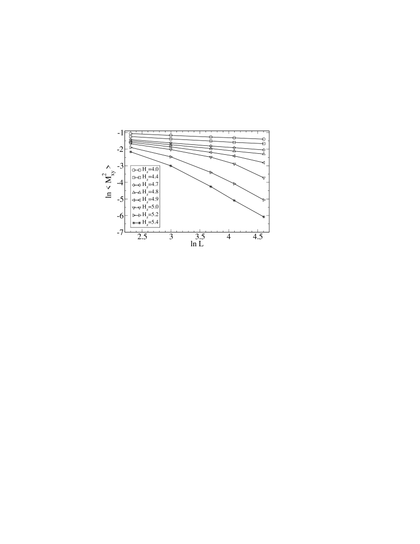
Figure 6: Logarithm of the transverse sublattice magnetization $<M_{xy}^{2}>$ versus the logarithm of the system size $L$ at fixed temperature $k_{B}T=0.6$ and for various fields $H_{z}$, close to the boundary between the spin-flop and the disordered phase.

The Kosterlitz-Thouless character of the transition between the spin-flop and the paramagnetic phases is also reflected in the thermal behavior of the specific heat $C$, which displays a non-critical maximum close to, but not exactly at the transition. Of course, from simulational data one cannot identify the expected essential singularity of $C$ at the transition.

IV Effects of defects

As discussed before,ls experiments on La₅Ca₉Cu₂₄O₄₁ in a field $H_{z}$ along the easy axis provide no evidence for a sharp transition from the antiferromagnetic to the spin-flop phase. Instead, when fixing the temperature and increasing the field, the antiferromagnetic phase eventually becomes unstable against the disordered phase, and spin-flop structures seem to occur at higher fields only locally as indicated by a quite large, but non-critical maximum in the susceptibility.am ; rk The reason for this experimentally observed behavior is not understood yet. Tentatively, one possible explanation invokes the holes or defects,spbk which may drive the transition and suppress the spin-flop phase.

In the following, we shall explore this possibility by extending the classical variant of the anisotropic Heisenberg model of Matsuda et al. by adding defects as described in Sec. II. Actually, ten percent of the lattice sites will be occupied by these spinless, mobile defects, in accordance with the experiments.nu We neglect the quantum nature of the holes and do not, e.g., include a kinetic energy or “hopping” term in the Hamiltonian as one would normally expect in the case of a doped quantum antiferromagnet. Of course, quantum effects may play an important role for the phase behavior of the doped model. E.g., quantum fluctuations lead to a non-zero mobility of the holes even at $T=0$ where our spinless defects are static due to the absence of thermal fluctuations. Nevertheless, our classical description is believed to provide some guidance to novel effects induced by the holes.

Without external field ($H_{z}=0$) in the ground state ($T=0$), the defects will form straight stripes perpendicular to the chains. Due to the next-nearest neighbor interactions, $J_{c2}$ and $J_{ac2}$, the stripes are bunched with two consecutive defects in a chain keeping the minimum distance of two lattice spacings with one spin in between the two defects. Such a bunching did not occur in the related Ising description,spbk where only nearest-neighbor couplings were assumed. In any event, the bunching may be suppressed, for example, by a pinning of the defects or repulsive interactions between the defects. The spins, in the ground state, are oriented along the $z$ axis with an antiferromagnetic ordering from chain to chain, as in the case without defects.

At low temperatures, the bunching dominates the typical equilibrium configurations, as illustrated in Fig. 7a.

Figure 7: Typical low temperature Monte Carlo equilibrium configurations showing (a) at $k_{B}T=0.3$, the bunching of defect lines, and (b) at $k_{B}T=0.6$, the onset of debunching, both for systems of size $L=40$. The open circles denote the mobile defects, while the arrows symbolize the $z$–components $S_{lm}^{z}$ of the spins.

Upon increasing the temperature, the stripes tend to debunch, thereby gaining entropy, see Fig. 7b. The debunching is reflected by a steep decrease in the density of defect pairs, i.e. consecutive defects in the same chain separated by merely one spin. The pronounced drop takes place in a rather narrow range of temperatures at roughly $k_{B}T\approx 0.55$. However, the debunching seems to be a gradual, smooth process, without any thermal singularities.

A phase transition occurs at $k_{B}T_{c}\approx 0.7$, i.e. at a significantly lower temperature than in the absence of defects. At the transition, the defect stripes destabilize. As for the Ising model with mobile defects, the stripe instability may be inferred from the average minimal distance $d_{a}$ between each defect in chain $m$, at position $(l_{d},m)$, and those in the next chain, at $(l_{d}^{\prime},m+1)$, defined by spbk ; hs

$$d_{a}=\sum\limits_{l_{d}}\langle\min|l_{d}-l_{d}^{\prime}|\rangle/N_{d},$$ (10)

dividing the sum by the number $N_{d}$ of defects. This quantity increases rapidly at the transition. The transition is also marked in the simulations by a pronounced peak in the specific heat and a drastic decrease in the sublattice magnetization, which is expected to vanish at $T\geq T_{c}$ in the thermodynamic limit.

Applying an increasing external field $H_{z}>0$ along the easy axis, the results of the ground state calculation (for even numbers of at least four defects per chain) may be summarized as follows. First, one has to distinguish two fields $H_{z}^{(1)}$ and $H_{z}^{(2)}$. For $0<H_{z}<H_{z}^{(1)}$ one keeps the same antiferromagnetic structure with bunched defect stripes as in the case of vanishing field. Then, for $H_{z}^{(1)}<H_{z}<H_{z}^{(2)}$, precisely one additional spin (pointing along the field direction) is inserted between two consecutive defects in every other chain, see Fig. 8a.

Figure 8: Illustration of the ground state configurations in an external field $H_{z}>0$ for a system with four defects per chain; for (a) $H_{z}^{(1)}<H_{z}<H_{z}^{(2)}$, and (b) $H_{z}^{(2)}<H_{z}<H^{\mathrm{sf}}$.

This configuration becomes unstable at $H_{z}=H_{z}^{(2)}$, and now an additional spin pointing in the $z$ direction is inserted between two consecutive defects in every chain (Fig. 8b). For simplicity and by analogy to the Ising case,spbk we refer to these two ground state configurations as ”zig-zag” structures. The two fields $H_{z}^{(1)}$ and $H_{z}^{(2)}$ are readily found to be given by $H_{z}^{(1)}=-J_{ac2}+J_{c2}/2$ and $H_{z}^{(2)}=2H_{z}^{(1)}$. Inserting the values of the interaction constants (see Sec. II) one obtains $H_{z}^{(1)}=0.4305$ and $H_{z}^{(2)}=0.861$. Note that broader regions of ”inserted” spins are, however, not favored energetically even when increasing the field. Instead, for larger fields, eventually a spin-flop transition occurs at $H^{\mathrm{sf}}$, followed by a ferromagnetic structure at higher fields, as in the case without defects.

The zig-zag structures lead to a stepwise increase in the total magnetization, which gives rise to rather small maxima in the susceptibility $\chi^{z}$ at low temperatures, as depicted in Fig. 9. One observes a small, non-critical peak at $H_{z}\approx 0.9$, which is the remnant of the transition at $T=0$ between the two zig-zag structures depicted in Fig. 8. Moreover, a very weak, non-critical maximum can be identified at $H_{z}\approx 0.5$ (see inset). This peak is associated with the zig-zag structure of Fig. 8a. At higher fields, a pronounced peak occurs signaling the transition to the spin-flop phase.

Figure 9: Susceptibility $\chi^{z}$ as a function of the magnetic field $H_{z}$ at fixed temperature $k_{B}T=0.3$, for a system of size $L=40$. The inset shows the existence of a very weak maximum at $H_{z}\approx 0.5$.

We found, however, no evidence for a phase transition at finite temperatures associated with the small peaks in $\chi^{z}$. Instead, upon increasing the field, straight stripes seem to transform gradually into zig-zag stripes, as for the Ising model with mobile defects.mh The first peaks already vanishes at about $k_{B}T\approx 0.3$, and the position of the second small peak shifts to somewhat higher fields and gets less pronounced as the temperature is increased. It disappears at about $k_{B}T\approx 0.5$, possibly due to the debunching. Obviously, the occurrence of zig-zag structures cannot be identified with the phase transition in La₅Ca₉Cu₂₄O₄₁ observed well below the onset of spin-flop structures.

Indeed, the anisotropic Heisenberg model with mobile defects still displays, at low temperatures, a sharp transition from the antiferromagnetic phase, with straight or zig-zag defect stripes, to a spin-flop phase, as signaled by a delta-like peak in the susceptibility $\chi^{z}$ (see Fig. 9). The topology of the phase diagram in the $(T,H_{z})$ plane seems to resemble that in the absence of defects, see Figs. 2a and 2b. Actually, at the triple point (or critical end point) between the antiferromagnetic, spin-flop and paramagnetic phases, located roughly at $(k_{B}T=0.5,H_{z}=1.7)$, the, presumably, non-critical debunching line seems to meet as well. However, we did not attempt to map the phase diagram accurately, because obviously the introduction of defects does not suffice to reconcile the experimental findings on La₅Ca₉Cu₂₄O₄₁, showing no direct transition from the antiferromagnetic to the spin-flop phase. In fact, the possible destruction of the spin-flop phase by the instability of the defect stripes tends to be hindered by the bunching of the stripes. Further investigations are desirable, but beyond the scope of the present study.

V Summary

We have analysed in detail a classical variant of a two-dimensional Heisenberg antiferromagnet with weak, uniaxial anisotropy proposed by Matsuda et al. to reproduce spin-wave dispersions measured in the magnet La₅Ca₉Cu₂₄O₄₁. In particular, we determined the phase diagrams of the model applying fields parallel, $H_{z}$, and perpendicular, $H_{x}$, to the easy axis of the spin anisotropy.

In the case of a transverse field $H_{x}$ (perpendicular to the easy axis), the transition from the antiferromagnetic phase to the paramagnetic phase belongs to the Ising universality class. The phase diagram in the case of a field $H_{z}$ pointing along the easy axis consists of the antiferromagnetic, the spin-flop, and the disordered (paramagnetic) phases. Extensive analyses have been performed to locate the phase boundaries, partly motivated by conflicting analyses of related models. Indeed, our analysis, studying especially the Binder cumulant and the transverse sublattice magnetization, allows one to locate reasonably well both the tricritical point on the phase boundary between the antiferromagnetic and the paramagnetic phases as well as the critical end point between these two phases and the spin-flop phase. Quantum effects seem to play no essential role for the topology of the phase diagram, which is in qualitative disagreement with experimental observations on La₅Ca₉Cu₂₄O₄₁.

We extended the classical variant of the model of Matsuda et al. by including spinless mobile defects mimicking the holes in La₅Ca₉Cu₂₄O₄₁, thereby following previous suggestions on a related Ising model. In the antiferromagnetic phase, the defects, at low temperatures and low fields, are found to form stripes as in the corresponding Ising case. However, due to next-nearest neighbor couplings, the stripes tend to bunch. The debunching, occurring at higher temperatures, seems to be non-critical, albeit it takes place in a rather narrow temperature range. A phase transition at which the antiferromagnetic order is destroyed is driven by a destruction of the defect stripes loosing their coherency at the transition.

The model with defects has also been studied in the presence of a field along the easy axis. There, a spin-flop phase is observed as well, separated from the antiferromagnetic phase presumably by a transition of first order. Therefore, we conclude that adding the mobile defects is not sufficient to reconcile model properties with experimental findings ruling out a direct transition from the antiferromagnetic to the spin-flop phase. Perhaps a destruction of the spin-flop phase may occur when the bunching is suppressed.

However, when interpreting our findings for the model with defects one should keep in mind that our description of the holes is a purely classical one. Quantum fluctuations reduce the clustering tendency of the holes and may also destroy the bunched structures that we find from our classical ground state analysis. Thus the role of quantum effects should certainly be investigated more carefully when comparing with actual experiments.

In any event, the models display various interesting behavior, and they may well contribute to arriving at a really satisfying theoretical description of the intriguing experimental observations on the La₅Ca₉Cu₂₄O₄₁ magnets. Moreover, the methods used in our study may be helpful in analysing phase diagrams of other two-dimensional weakly anisotropic Heisenberg antiferromagnets.

- (1) S. A. Carter, B. Batlogg, R. J. Cava, J. J. Krajewski, W. F. Peck Jr., and T. M. Rice, Phys. Rev. Lett. 77, 1378 (1996).
- (2) M. Matsuda, K. Katsumata, T. Yokoo, S. M. Shapiro, and G. Shirane, Phys. Rev. B 54, R15626 (1996).
- (3) Y. Mizuno, T. Tohyama, S. Maekawa, T. Osafune, N. Motoyama, H. Eisaki, and S. Uchida, Phys. Rev. B 57, 5326, (1998).
- (4) M. Matsuda, K. M. Kojima, Y. J. Uemura, J. L. Zarestky, K. Nakajima, K. Kakurai, T. Yokoo, S. M. Shapiro, and G. Shirane, Phys. Rev. B 57, 11467 (1998).
- (5) U. Ammerahl, B. Büchner, C. Kerpen, R. Gross, and A. Revcolevschi, Phys. Rev. B 62, R3592 (2000).
- (6) V. Kataev, K.-Y. Choi, M. Grüninger, U. Ammerahl, B. Büchner, A. Freimuth, and A. Revcolevschi, Phys. Rev. Lett. 86, 2882 (2001).
- (7) M. Windt, M. Grüninger, T. Nunner, C. Knetter, K. P. Schmidt, G. S. Uhrig, T. Kopp, A. Freimuth, U. Ammerahl, B. Büchner, and A. Revcolevschi, Phys. Rev. Lett. 87, 127002 (2001).
- (8) R. Klingeler, PhD thesis, RWTH Aachen (2003).
- (9) M. Matsuda, K. Kakurai, J. E. Lorenzo, L. P. Regnault, A. Hiess, and G. Shirane, Phys. Rev. B 68, 060406(R) (2003).
- (10) A. Cuccoli, T. Roscilde, V. Tognetti, R. Vaia, and P. Verrucchi, Phys. Rev. B 67, 104414 (2003).
- (11) P. A. Serena, N. García, and A. Levanyuk, Phys. Rev. B 47, 5027 (1993).
- (12) N. Nücker, M. Merz, C. A. Kuntscher, S. Gerhold, S. Schuppler, R. Neudert, M. S. Golden, J. Fink, D. Schild, S. Stadler, V. Chakarian, J. Freeland, Y. U. Idzerda, K. Conder, M. Uehara, T. Nagata, J. Goto, J. Akimitsu, N. Motoyama, H. Eisaki, S. Uchida, U. Ammerahl, and A. Revcolevschi, Phys. Rev. B 62, 14384 (2000).
- (13) W. Selke, V. L. Pokrovsky, B. Büchner, and T. Kroll, Eur. Phys. J. B 30, 83 (2002).
- (14) M. Holtschneider and W. Selke, Phys. Rev. E 68, 026120 (2003).
- (15) R. Leidl and W. Selke, Phys. Rev. B 69, 056401 (2004).
- (16) M. E. Fisher and D. R. Nelson, Phys. Rev. Lett. 32, 1350 (1974).
- (17) D. P. Landau and K. Binder, Phys. Rev. B 24, 1391 (1981).
- (18) B. V. Costa and A. S. T. Pires, J. Magn. Magn. Mat. 262, 316 (2003).
- (19) G. Schmid, S. Todo, M. Troyer, and A. Dorneich, Phys. Rev. Lett. 88, 167208 (2002).
- (20) H. J. M. de Groot and L. J. de Jongh, Physica B 141, 1 (1986).
- (21) H. Rauh, W. A. C. Erkelens, L. P. Regnault, J. Rossat–Mignod, W. Kullmann, and R. Geick, J. Phys. C 19, 4503 (1986).
- (22) R. van de Kamp, M. Steiner, and H. Tietze–Jaensch, Physica B 241, 570 (1998).
- (23) K. Binder, Z. Phys. B 43, 119 (1981).
- (24) J. M. Kosterlitz and D. J. Thouless, J. Phys. C 6, 1181 (1973).
- (25) M. Holtschneider, R. Leidl, and W. Selke, submitted to J. Magn. Magn. Mat.
- (26) G. Kamieniarz and H. W. J. Blöte, J. Phys. A 26, 201 (1993).
- (27) D. Nicolaides and A. D. Bruce, J. Phys. A 21, 233 (1988).
- (28) X.S. Chen and V. Dohm, cond-mat/0408511 (2004).
- (29) M. Holtschneider, Diploma thesis, RWTH Aachen (2003).