Temperature Anisotropy in a Driven Granular Gas

Abstract

When smooth granular material is fluidized by vertically shaking a container, we find that the temperature in the direction of energy input always exceeds the temperature in the other directions. An analytical model is presented which shows how the anisotropy can be traced back to the inelasticity of the interparticle collisions and the collisions with the wall. The model compares very well with molecular dynamics simulations. It is concluded that any non-isotropic driving of a granular gas in a steady state necessarily causes anisotropy of the granular temperature.

As compared to an ordinary, molecular gas, the hallmark of a granular gas is its permanent dissipation of energy due to inelastic collisions. Whereas an isolated molecular gas will sustain its motion for an infinite amount of time, the only true equilibrium state of granular matter is the one where it is at rest. Hence a steady supply of energy is required to keep a granular gas alive, giving rise to prototypical non-equilibrium systems with many striking phenomena goldhirsch03 ; weele03 . The one addressed in this Letter is the crucial temperature anisotropy within a granular gas. It is observed to be a significant effect in both numerical simulations mcnamara98 ; barrat02 ; herbst04 ; brey98cub ; krouskop03 ; krouskop03b and experiments wildman00 ; yang02 ; kudrolli01 ; kudrolli03 . Although it has been studied in the context of a random restitution coefficient model barrat01 ; barrat03 , a theoretical explanation is still lacking. Here we provide such an explanation, in which for analytical convenience we will restrict ourselves to a dilute granular gas, fluidized by vertically vibrating a container.

So what causes the anisotropy? We approach this question by a theoretical model in combination with event driven molecular dynamics (MD) simulations, and show that the anisotropy results from the following characteristic feature of such a gas: The distribution of energy from the vibrating bottom towards the horizontal directions occurs through the very same mechanism that also constitutes one of the major sources of energy dissipation, i.e., the collisions between the particles. This result carries over to any granular gas with a non-isotropic energy source.

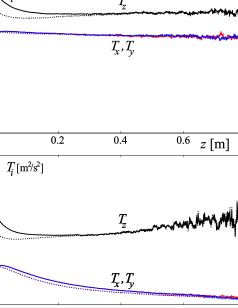
Figure 1: Solid lines: Temperature components (1) from MD simulations of the driven granular gas model as specified in the main text with sinusoidal driving and parameters $f=72.648$ Hz, $a=1.00$ mm, $N=50$, $r_{\!p}=1.18$ mm, and $L=2.265$ cm. (a): $e_{p}=0.9$ and $e_{w}=1$ (reflective sidewalls). (b): $e_{p}=0.95$ and $e_{w}=0.95$ (dissipative sidewalls). Dashed lines: Counting only particles that move downward, i.e. restricting the average in (1) to negative $v_{z}$-values. At large $z$ the statistics deteriorates since particles rarely reach such heights. The curves $T_{x}(z)$ and $T_{y}(z)$ practically coincide.

The setup we will consider in our present work consists of a granular gas in a container with a square-shaped bottom of side length $L$ in the $x$-$y$-plane and infinitely high, vertical side-walls. Gravity acts with $g=9.81$ m/s² and the gas is fluidized by vertical vibrations of the bottom about $z=0$ with amplitude $a$ and frequency $f$ – typically of triangular (piecewise linear, symmetric) or sinusoidal shape. The gas consists of $N$ identical hard spheres with radius $r_{\!p}$ and mass $m$. We restrict ourselves to the case mcnamara98 ; sela98 ; brey98 ; baldassari01 ; brey01 ; eggers99 ; soto99 that only normal restitution goldhirsch03 ; weele03 contributes to the dissipative processes, with restitution coefficients $e_{p}$ for particle-particle and $e_{w}$ for particle-wall collisions, while collisions with the vibrating bottom are taken to be perfectly elastic.

After initial transients have died out, we expect (and observe) a stationary probability distribution $\rho({\mbox{\boldmath$r$}},{\mbox{\boldmath$v$}})$ of the particle positions ${\mbox{\boldmath$r$}}:=(x,y,z)$ and velocities ${\mbox{\boldmath$v$}}:=(v_{x},v_{y},v_{z})$. The quantities of central interest are the temperature components

$$T_{i}(z):=\frac{m}{k}\,\langle v_{i}^{2}\rangle$$ (1)

where $i\in\{x,y,z\}$ and $k$ is Boltzmann’s constant. This $T_{i}(z)$ is directly proportional to the average kinetic energy of the particles in a horizontal layer at height $z$ in either of the three spatial directions $i$.

In evaluating our MD simulations we replace ensemble averages in (1) by time averages (justified by ergodicity) and work in units with $m=1$ and $k=1$. A representative result is depicted in Fig. 1: As expected for symmetry reasons, the horizontal temperature components $T_{x}(z)$ and $T_{y}(z)$ are practically indistinguishable. In contrast, the vertical temperature component $T_{z}(z)$ is significantly larger than $T_{x}(z)$ and $T_{y}(z)$. For perfectly elastic particle-wall collisions (Fig. 1a) the $z$-dependence of the temperature components is very weak except for a region directly above the bottom. There, the energy-input by the driving leads to increased upward particle velocities, as shown by the dashed lines in (Fig. 1a). For inelastic particle-wall collisions (Fig. 1b) the $z$-dependence of the temperature components is more pronounced. Yet, in both cases the differences between vertical and horizontal temperatures are more important than the $z$-dependences.

Our theoretical analysis of the observed temperature differences starts with the well-known conservation laws of energy and momentum for a dilute granular gas, derived from Boltzmann’s equation sela98 ; brey98 ; baldassari01 . For a stationary system, they read, in terms of the local heat flux $\mathbf{J}({\mbox{\boldmath$r$}})$ and stress (or pressure) tensor $\mathbf{P}({\mbox{\boldmath$r$}})$:

$$\nabla\cdot\mathbf{J}({\mbox{\boldmath$r$}})=I({\mbox{\boldmath$r$}})\ ,\ \ \nabla\cdot\mathbf{P}({\mbox{\boldmath$r$}})=n({\mbox{\boldmath$r$}})\mathbf{f}({\mbox{\boldmath$r$}})\ .$$ (2)

Here, $I({\mbox{\boldmath$r$}})$ is the local energy dissipation rate per unit volume, $n({\mbox{\boldmath$r$}})$ is the local particle density, and the force $\mathbf{f}({\mbox{\boldmath$r$}})=-mg\mathbf{e}_{z}$. Integrating the first equation (2) over the container volume $V$ we obtain with Gauss’ theorem that the energy dissipation rate due to particle-particle collisions $Q_{pp}:=\int_{V}I({\mbox{\boldmath$r$}})\,d\mathbf{r}$ must be equal to the total flux of energy through the boundaries. The latter can be decomposed in the influx $Q_{in}:=L^{2}\,J_{z}(0)$ of energy through the vibrating bottom of area $L^{2}$ and the energy dissipation rate $Q_{w}$ due to particle-wall collisions. This gives

$$Q_{in}=Q_{pp}+Q_{w}.$$ (3)

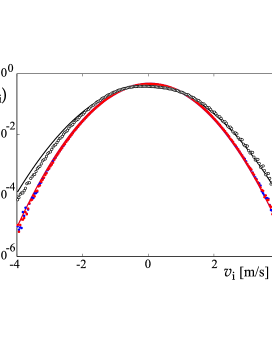
Figure 2: Horizontal (solid red and blue dots) and vertical (open, black dots) velocity distributions of particles in a layer between $z=0$ and $z=5$ mm obtained by MD simulations for the same system as in Fig. 1a but with $f=30$ Hz and $L=4.8$ cm. The solid lines are Gaussian fits f2 .

Crucial to the present model is that the temperature components $T_{i}$ defined in (1) are treated separately. To our knowledge, all existing theories for driven granular gases in a steady state without net flow of material are based upon the assumption of an isotropic temperature, and many of them also on isotropic stress sela98 ; brey98 ; baldassari01 ; brey01 ; f1 .

The temperature components $T_{i}$ are related to the diagonal elements of the stress tensor by a generalized ideal gas law $P_{ii}=nkT_{i}$ sela98 ; brey98 ; baldassari01 . Motivated by our MD simulations, we assume that each temperature component $T_{i}$ is approximately constant within the entire container volume (see also kumaran98 ; eggers99 ). Because of symmetry the stress tensor is diagonal and $T_{x}=T_{y}=:T_{\!h\!o\!r}$, with which the second equation (2) can now be readily integrated to yield

$$n({\mbox{\boldmath$r$}})=\frac{Nmg}{L^{2}kT_{z}}\exp\left\{-\frac{mgz}{kT_{z}}\right\}\ .$$ (4)

Furthermore, as exemplified by Fig. 2, our MD simulations show that the particle velocity components can be assumed as Gaussian distributed in very good approximation for a wide range of parameter values olafsen99 ; f2 . All together, we thus arrive at the following approximative distribution function for particle position and velocity:

$$\rho({\mbox{\boldmath$r$}},{\mbox{\boldmath$v$}})=\frac{n({\mbox{\boldmath$r$}})\ m^{3/2}}{\sqrt{(2\pi k)^{3}T_{\!h\!o\!r}^{2}T_{z}}}\exp\!\left\{\!-\frac{m(v_{x}^{2}+x_{y}^{2})}{2kT_{\!h\!o\!r}}-\frac{mv_{z}^{2}}{2kT_{z}}\!\right\}\ .$$ (5)

The next main idea is to determine the two unknowns $T_{z}$ and $T_{\!h\!o\!r}$ in (5) by means of two energy balance relations. The first of them is (3). To obtain the second, we observe that particle-particle collisions not only cause energy dissipation but also a transfer of kinetic energy from the horizontal direction into the vertical direction, and vice versa. In the steady state the net effect must be an average loss of kinetic energy per time unit $Q_{z}$ in the vertical direction which is exactly balanced by the incoming energy flux $Q_{in}$ through the vibrating bottom:

$$Q_{in}=Q_{z}\ .$$ (6)

The remaining, rather technical task is to explicitly determine all the energy fluxes $Q$ appearing in (3) and (6) with the help of the approximation (5). In order to evaluate $Q_{z}$, we first note that the change of kinetic energy in the vertical direction in a single particle-particle collision is

$$q_{z}=\sum_{j=1}^{2}\frac{m}{2}\left(({\mbox{\boldmath$v$}}_{j}\cdot{\mbox{\boldmath$e$}}_{z})^{2}-({\mbox{\boldmath$v$}}^{*}_{j}\cdot{\mbox{\boldmath$e$}}_{z})^{2}\right)\ ,$$ (7)

where ${\mbox{\boldmath$v$}}_{j}$ and ${\mbox{\boldmath$v$}}^{*}_{j}$ are the velocities of the two colliding particles ($j=1,2$) before and after the collision, respectively. Due to our assumption that only normal restitution contributes to the dissipative processes, we have ${\mbox{\boldmath$v$}}^{*}_{j}={\mbox{\boldmath$v$}}_{j}+(-1)^{j}(1+e_{p})[({\mbox{\boldmath$v$}}_{1}-{\mbox{\boldmath$v$}}_{2})\cdot{\mbox{\boldmath$n$}}]{\mbox{\boldmath$n$}}/2$, where $n$ is the collision normal vector. To determine $Q_{z}$ one essentially has to introduce this result for ${\mbox{\boldmath$v$}}^{*}_{j}$ into (7) and then average according to (5). More precisely, first $q_{z}$ in (7) is multiplied by the collisional volume per unit time $(1/2)\pi(2r_{\!p})^{2}|{\mbox{\boldmath$v$}}_{2}-{\mbox{\boldmath$v$}}_{1}|\delta(|{\mbox{\boldmath$r$}}_{1}-{\mbox{\boldmath$r$}}_{2}|-2r_{\!p})$, where the factor $1/2$ arises since collisions only can happen if $({\mbox{\boldmath$v$}}_{2}-{\mbox{\boldmath$v$}}_{1})\cdot{\mbox{\boldmath$n$}}<0$. Next we multiply with $(1/2)\rho({\mbox{\boldmath$r$}}_{1},{\mbox{\boldmath$v$}}_{1})\rho({\mbox{\boldmath$r$}}_{2},{\mbox{\boldmath$v$}}_{2})$ according to (5) and integrate over all ${\mbox{\boldmath$v$}}_{j}$ and ${\mbox{\boldmath$r$}}_{j}$ (within the container volume). The factor $1/2$ is needed since every collision appears twice in the above considerations. This gives, after a substantial amount of algebra:

$$Q_{z}\!\! = \!\!(1+e_{p})\,(Nr_{\!p}/L)^{2}g\sqrt{\pi mkT_{z}}\,F(T_{\!h\!o\!r}/T_{z})$$ (8)

$$F(\vartheta)\!\! := \!\!\int\limits_{0}^{\infty}\!ds\!\int\limits_{0}^{\infty}\!dt\,\sqrt{s+t}\,\frac{(8-4e_{p})s-(1+e_{p})t}{6\,\vartheta\sqrt{s}\,\exp\{s+t/\vartheta\}}\ .$$

A similar averaging of the total energy loss in a single particle-particle collision $q_{pp}=(m/2)\sum_{j=1}^{2}({\mbox{\boldmath$v$}}_{j}^{2}-({\mbox{\boldmath$v$}}^{*}_{j})^{2})$ yields

$$Q_{pp}\!\! = \!\!(1-e_{p}^{2})\,(Nr_{\!p}/L)^{2}g\sqrt{\pi mkT_{z}}\,G(T_{\!h\!o\!r}/T_{z})$$ (9)

$$G(\vartheta)\!\! := \!\!\int\limits_{0}^{\infty}\!ds\!\int\limits_{0}^{\infty}\!dt\,\frac{[s+t]^{3/2}}{\vartheta\sqrt{s}\,\exp\{s+t/\vartheta\}}\ .$$

In the same spirit one can evaluate the total dissipation rate due to particle-wall collisions $Q_{w}$ with the result

$$Q_{w}=4\,(1-e_{w}^{2})\,N\,(kT_{\!h\!o\!r})^{3/2}/(L\sqrt{2\pi m})$$ (10)

Finally, a somewhat lengthy but straightforward calculation yields the following expression for the energy input rate at the perfectly elastic, vibrating bottom of the container:

$$Q_{in}=2\,N\,g\,m^{3/2}\,u^{2}\psi(\gamma)/\sqrt{\pi kT_{z}}$$ (11)

where $\gamma:=\sqrt{2kT_{z}/mu^{2}}$, $u=:\pi\sqrt{2}\,af$ for sinusoidal driving of the bottom, and $u:=4\,af$ for triangular driving. In both cases, for large $\gamma$ (which is the typical situation in the dilute systems under study) the function $\psi(\gamma)$ approaches unity f3 .

In the absence of wall dissipation ($e_{w}=1$), Eqs. (3), (6), (8)-(11) imply

$$F(T_{\!h\!o\!r}/T_{z})=(1-e_{p})G(T_{\!h\!o\!r}/T_{z})\ ,\ \ [e_{w}=1]\ .$$ (12)

Closer inspection shows that for any $0\leq e_{p}<1$ a unique solution $0\leq T_{\!h\!o\!r}/T_{z}<1$ of (12) exists. In particular, for small $1-e_{p}$ one finds the leading order asymptotics

$$T_{\!h\!o\!r}/T_{z}=1-(5/2)\,(1-e_{p})\ ,\ \ [e_{w}=1]\ .$$ (13)

Thus for $e_{p}<1$ and perfectly reflecting walls, the model predicts that the horizontal temperature $T_{\!h\!o\!r}$ is always smaller than the vertical temperature $T_{z}$. Moreover, the ratio $T_{\!h\!o\!r}/T_{z}$ solely depends on $e_{p}$ but not on any details of driving shape and strength, particle density, particle size, or compartment geometry. The comparison with MD simulations in Fig. 3 is excellent. The inset of Fig. 3 shows that the remaining deviations can largely be attributed to finite size effects.

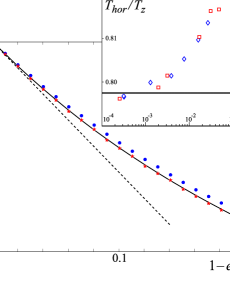
Figure 3: Ratio of horizontal and vertical temperatures versus particle-particle restitution coefficient. Solid line: Theoretical prediction (12). Dashed line: Theoretical asymptotic behavior (13). Symbols: MD simulations for the same system as in Fig. 1a with $N=20$ ($\star$) and $N=50$ ($\bullet$) particles. For $e_{p}\not=0.9$, a different choice for the frequency $f$ such that the $T_{z}$ was (approximately) the same for all $e_{p}$. Inset: Same, but for fixed $e_{p}=0.9$ and variable local solid fraction $\sigma:=(4/3)\pi r_{\!p}^{3}\max[n({\bf r})]$, either by varying particle number $N$ ($\Diamond$, at $r=1.18$ mm) or radius $r_{\!p}$ ($\Box$, at $N=50$).

In the general case one obtains two transcendental, algebraic equations for the two unknowns $T_{\!h\!o\!r}$ and $T_{z}$ by introducing (8)-(11) into (3) and (6). While existence and uniqueness of solutions can still be demonstrated analytically, their quantitative determination is only possible numerically. An example is depicted in Fig. 4, comparing very well with MD simulations. As expected, dissipative walls tend to reduce the horizontal temperature $T_{\!h\!o\!r}$ since they add a source of dissipation for the horizontal kinetic energy. If we increase the particle number, the gas becomes more dense, and the number of particle-particle collisions will increase much faster than the number of particle-wall collisions. Therefore, $T_{\!h\!o\!r}$ will first increase, in sharp contrast to the overall temperature $[T_{z}+2T_{\!h\!o\!r}]/3$ which must decrease with increasing particle density. Eventually, particle-particle collisions will dominate the system, and $T_{\!h\!o\!r}/T_{z}$ will asymptotically tend to the value it would have with reflecting walls.

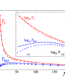
Figure 4: Horizontal (blue) and vertical (red) temperatures versus particle number. Lines: Theoretical predictions from (3), (6), (8)-(11) for triangular driving and parameters $f=30$ Hz, $a=1.00$ mm, $r_{\!p}=1.18$ mm, $L=4.8$ cm, $e_{p}=0.95$ and $e_{w}=0.95$. Symbols: MD simulations. Inset: Same data in a log-log plot.

In conclusion, we have numerically observed large differences between the vertical and horizontal temperatures in vertically driven granular gases subjected to gravity. We introduced a theoretical model based on an approximative Maxwell-Boltzmann distribution with anisotropic but homogeneous temperature (5), justified by our MD simulations. Both for reflecting and dissipative walls of the container we find that the theoretical model gives good quantitative agreement with the simulations.

The difference of the horizontal and vertical temperatures from the isotropic value is a significant correction, at least of the same order as those resulting from taking into account the non-constancy of the temperature and density profiles, or from embedding Chapman-Enskog corrections to the velocity distributions into the theoretical framework sela98 ; brey98 .

At the root of the temperature anisotropy lies the fact that the transfer of kinetic energy between different spatial directions and its dissipation arise out of the same mechanism: the collisions between the particles. Thus, the anisotropy of the temperature is a necessary consequence of the anisotropy of the driving. The present work indicates that one may obtain an improved hydrodynamic description for dilute granular gases by starting out from an anisotropic velocity distribution (instead of an isotropic one) in deriving hydrodynamics equations from Boltzmann’s equation.

The basic concept of the model applies to any situation in which the energy-input in a granular gas is anisotropic, always predicting a higher kinetic energy content in the main direction of energy-input.

- (1) I. Goldhirsch, Annu. Rev. Fluid Mech. 35, 267 (2003).
- (2) K. van der Weele, R. Mikkelsen, D. van der Meer, and D. Lohse, in The Physics of Granular Media, D. Wolf and H. Hinrichsen (ed.), vol. in press (Wiley-VCH, 2004).
- (3) S. McNamara and S. Luding, Phys. Rev. E 58, 813 (1998).
- (4) J. Brey and D. Cubero, Phys. Rev. E 57, 2019 (1998).
- (5) A. Barrat and E. Trizac, Phys. Rev. E 66, 051303 (2002).
- (6) P.E. Krouskop and J. Talbot, cond-mat/0303263 (preprint, 2003).
- (7) P.E. Krouskop and J. Talbot, cond-mat/0312530 (preprint, 2003).
- (8) O. Herbst, P. Müller, M. Otto, and A. Zippelius, cond-mat/0402104 (preprint, 2004).
- (9) X. Yang, C. Huan, D. Candela, R.W. Mair, and R.L. Walsworth, Phys. Rev. Lett. 88, 044301 (2002).
- (10) R.D. Wildman and J.M. Huntley, Powder Technology 113, 14 (2000).
- (11) D.L. Blair and A. Kudrolli, Phys. Rev. E 64, 050301 (2001).
- (12) D.L. Blair and A. Kudrolli, Phys. Rev. E 67, 041301 (2003).
- (13) A. Barrat, E. Trizac, and J. N. Fuchs, Eur. Phys. J. E 5, 161 (2001).
- (14) A. Barrat and E. Trizac, Eur. Phys. J. E 11, 99 (2003).
- (15) N. Sela and I. Goldhirsch, J. Fluid Mech. 361, 41 (1998).
- (16) J.J. Brey, J.W. Dufty, C.S. Kim, and A. Santos, Phys. Rev. E 58, 4638 (1998).
- (17) A. Baldassarri, U. Marini Bettolo Marconi, A. Puglisi, and A. Vulpiani, Phys. Rev. E 64, 011301 (2001).
- (18) J.J. Brey, M.J. Ruiz-Montero, and F. Moreno, Phys. Rev. E 63, 061305 (2001).
- (19) J. Eggers, Phys. Rev. Lett. 83, 5322 (1999).
- (20) R. Soto, M. Mareschal, and D. Risso, Phys. Rev. Lett. 83, 5003 (1999).
- (21) V. Kumaran, Phys. Rev. E 57, 5660 (1998).
- (22) J.S. Olafsen and J.S. Urbach, Phys. Rev. E 60, R2468 (1999).
- (23) C.S. Campbell and A. Gong, J. Fluid Mech. 164, 107 (1986).
- (24) I. Goldhirsch and N. Sela, Phys. Rev. E 54, 4458 (1996).
- (25) J.T. Jenkins and M.W. Richman, J. Fluid Mech. 192, 313 (1988).
- (26) V. Kumaran, Phys. Rev. Lett. 82, 3248 (1999).
- (27) J.J. Brey, M.J. Ruiz-Montero, and F. Moreno, Phys. Rev. E 62, 5339 (2000).
- (28) Only in the context of the normal-stress differences observed in steady plane Couette flow of granular material campbell86 , an anisotropic stress tensor goldhirsch96 or Maxwell-Boltzmann velocity distribution jenkins88 has been used.
- (29) In brey00 ; kumaran99 , large deviations from Gaussian velocity distributions, especially near the vibrating bottom, have been reported. Our simulations show that they are rooted in the discontinuous, saw-tooth shape of the vibrations considered in brey00 ; kumaran99 . This is the main reason that we focus on continuous shapes of the driving in the present work.
- (30) For triangular driving we have derived the exact result . For sinusoidal driving we were only able to show that for .