Andreev interference in adiabatic pumping

Abstract

Within the scattering approach, we develop a model for adiabatic quantum pumping in hybrid normal/superconductor systems where several superconducting leads are present. This is exploited to study Andreev-interference effects on adiabatically pumped charge in a 3-arm beam splitter attached to one normal and two superconducting leads with different phases of the order parameters. We derive expressions for the pumped charge through the normal lead for different parameters for the scattering region, and elucidate the effects due to Andreev interference. In contrast to what happens for voltage-driven transport, Andreev interference does not yield in general a pumped current which is a symmetric function of the superconducting-phase difference.

Introduction. Pumping consists in the transport of particles obtained, in absence of a transport voltage, by varying in time some properties of a mesoscopic conductor. If the time scale for the variation of the scattering matrix describing the conductor is larger than the transport time, then the pumping is adiabatic and the number of particles transferred per period does not depend on the detailed time evolution of the scattering matrix but only on geometrical properties of the pumping cycle brouwer .

Adiabatic pumping has attracted a vast interest, and different aspects of this phenomenon have been addressed makhlin ; levitov ; levinson ; aleiner ; moskalets ; butti as, for example, the counting statistics of the pumped current, the generalization to multi-terminal geometries and the question of phase coherence. The idea of adiabatic pumping has been combined with other phenomena typical of mesoscopic physics, like spin-dependent transportmucciolo ; spinpump ; watson , Kondo physicswangpumping ; aono , Luttinger-liquid physicscitro , and Quantum Hall effectquantumhall . So far, there have been only few investigations of adiabatic pumping in normal/superconductor hybrid structures. Zhouzhoucondmat has considered the pumped current due to the time-modulation of the superconducting correlations induced in the normal region. Wang et al.wangapl have studied the combined effect of pumping and Andreev reflection in a system with only one single-mode superconducting lead, finding up to a fourfold enhancement of the pumped current due to the interplay of Andreev and normal reflection. The generalization to a multi-mode superconducting lead was done by Blaauboerblaauboer .

In this paper we explore the physics of adiabatic pumping in the presence of several superconducting leads. In particular, we want to study Andreev interference in adiabatic pumping. Andreev interferometers have been intensively investigated in the past both in the diffusive limit hekking_93 ; hui_93 ; nazarov_94 ; zaitsev_94 ; nazarov_96 ; volkov_96 , and in the ballistic onenakano ; takagi (for an extended list of references see, for example, Ref. lambert_98 ). In a standard Andreev interferometer (as those considered in Refs. hekking_93 ; nazarov_94 ; nazarov_96 ; volkov_96 ; nakano ; takagi ) transport is driven by an applied voltage. In the present work, we study the problem of an Andreev interferometer when transport is induced by adiabatic pumping.

The paper is organized as follows: we start by deriving a formula for the current pumped through a normal lead in the presence of several other normal and superconducting leads; then we apply the formalism to a fork-shaped structure which exhibits Andreev interference.

Formalism. We consider a system consisting of $P$ normal and $Q$ superconducting leads connected to a generic scattering region characterized by its scattering matrix $\mathcal{S}$ (matrices are in boldface). The different superconductors are described by a constant pair potential $\Delta_{m}=|\Delta_{m}|\exp{(i\Phi_{m})}$, where $m=1,...,Q$ labels the superconducting leads. We note that when all leads are in the normal state we can write the scattering matrix as

$$\mbox{\boldmath$S$}_{\text{N}}=\left(\begin{array}[]{cc}\mbox{\boldmath$R$}(\epsilon)&\mbox{\boldmath$T$}^{\prime}(\epsilon)\\ \mbox{\boldmath$T$}(\epsilon)&\mbox{\boldmath$R$}^{\prime}(\epsilon)\end{array}\right),$$ (1)

where $R$ is a $P\times P$ matrix containing the scattering amplitudes between the normal terminals; $\mbox{\boldmath$R$}^{\prime}$ is a $Q\times Q$ matrix containing the scattering amplitudes between the superconducting terminals; $T$ is a $Q\times P$ matrix describing the scattering between the normal leads and the superconducting ones; and $\mbox{\boldmath$T$}^{\prime}$ is $P\times Q$ matrix describing the scattering between the superconducting leads and the normal ones. The energy $\epsilon$ is measured with respect to the Fermi energy. Writing the scattering matrix as in Eq. (1) makes evident that the system is equivalent to one consisting only of a normal lead with $P$ modes and a superconducting lead with $Q$ modes, each mode in the superconducting lead having its own pair potential $\Delta_{m}$. We can now write the scattering matrix for the hybrid normal–superconductor system in Nambu space:

$$\mbox{\boldmath$\mathcal{S}$}=\left(\begin{array}[]{cc}\mbox{\boldmath$\mathcal{R}$}_{\text{ee}}(\epsilon)&-{\mbox{\boldmath$\mathcal{R}$}_{\text{he}}}^{*}(-\epsilon)\\ \mbox{\boldmath$\mathcal{R}$}_{\text{he}}(\epsilon)&{\mbox{\boldmath$\mathcal{R}$}_{\text{ee}}}^{*}(-\epsilon)\end{array}\right),$$ (2)

where the submatrices are obtained composing the matrix $\mbox{\boldmath$S$}_{\text{N}}$ with the scattering matrix $\mbox{\boldmath$S$}_{\text{NS}}$ of a perfect NS multichannel interface beenakker . The latter is a diagonal matrix of Andreev reflection amplitudes which can be written, under the Andreev approximation, as $\mbox{\boldmath$S$}_{\text{NS}}=\mbox{\boldmath$\alpha$}~{}\mbox{\boldmath$e^{-i\Phi}$}$, where $\alpha$ is a diagonal matrix whose elements are $\exp[-i\text{Arcos}(\epsilon/|\Delta_{m}|)]$ and $e^{-i\Phi}$ is a diagonal matrix of elements $\exp[-i\Phi_{m}]$. As a result:

$$\mathbf{\mbox{\boldmath$\mathcal{R}$}_{\text{ee}}}(\epsilon) = \mbox{\boldmath$R$}(\epsilon)+$$ (3a)

$$\mbox{\boldmath$T$}^{\prime}(\epsilon)\mbox{\boldmath$\alpha e^{i\Phi}$}{\mbox{\boldmath$R$}^{\prime}}^{*}(-\epsilon)\mbox{\boldmath$\alpha$}\mbox{\boldmath$e^{-i\Phi}$}\mbox{\boldmath$M$}(\epsilon)\mbox{\boldmath$T$}(\epsilon)$$

$$\mbox{\boldmath$\mathcal{R}$}_{\text{he}}(\epsilon) = {\mbox{\boldmath$T$}^{\prime}}^{*}(-\epsilon)\mbox{\boldmath$\alpha$}\mbox{\boldmath$e^{-i\Phi}$}\mbox{\boldmath$M$}(\epsilon)\mbox{\boldmath$T$}(\epsilon)$$ (3b)

with

$$\mbox{\boldmath$M$}(\epsilon)=\left[\mathbf{1}-\mbox{\boldmath$R$}^{\prime}(\epsilon)\mbox{\boldmath$\alpha e^{i\Phi}$}{\mbox{\boldmath$R$}^{\prime}}^{*}(-\epsilon)\mbox{\boldmath$\alpha e^{-i\Phi}$}\right]^{-1}.$$ (4)

In Eq. (2), $\mbox{\boldmath$\mathcal{R}$}_{\text{ee}}$ ($\mbox{\boldmath$\mathcal{R}$}_{\text{he}}$) is a $P\times P$ matrix of normal (Andreev) scattering amplitudes between the normal leads. Note that we have used the particle-hole symmetry, which yields $\mbox{\boldmath$\mathcal{R}$}_{\text{hh}}(\epsilon)=\mbox{\boldmath$\mathcal{R}$}^{*}_{\text{ee}}(-\epsilon)$ and $\mbox{\boldmath$\mathcal{R}$}_{\text{eh}}(\epsilon)=-\mbox{\boldmath$\mathcal{R}$}^{*}_{\text{he}}(-\epsilon)$.

By means of the scattering matrix Eq. (2), operating along the same lines of Refs. blaauboer ; buettiker_02 , we can write the charge pumped through any of the normal leads:

$$Q_{n}=\frac{e}{\pi}\int dX_{1}dX_{2}\sum_{l\in\text{Normal leads}}\Pi_{n,l}(X_{1},X_{2}),$$ (5)

where $X_{1}$, and $X_{2}$ are the two pumping fields, and

$$\Pi_{n,l}(X_{1},X_{2})=\int_{-\infty}^{\infty}d\epsilon\left(-\frac{\partial f}{\partial\epsilon}\right)\mbox{Im}\left\{\frac{\partial\left({\mbox{\boldmath$\mathcal{R}$}_{\text{ee}}}^{*}(\epsilon)\right)_{n,l}}{\partial X_{1}}\frac{\partial\left({\mbox{\boldmath$\mathcal{R}$}_{\text{ee}}(\epsilon)}\right)_{n,l}}{\partial X_{2}}-\frac{\partial\left({\mbox{\boldmath$\mathcal{R}$}_{\text{he}}}^{*}(\epsilon)\right)_{n,l}}{\partial X_{1}}\frac{\partial\left(\mbox{\boldmath$\mathcal{R}$}_{\text{he}}(\epsilon)\right)_{n,l}}{\partial X_{2}}\right\},$$ (6)

with $f(\epsilon)$ being the Fermi Dirac distribution. Although Eq. (6) is valid at finite temperature, in the rest of the paper we will restrict ourselves to zero temperature.

Andreev interferometers. We, now, apply the formalism developed above to an example of an Andreev interferometer. The most simple system which allows us to investigate pumping with different superconductors consists of a 3-arm beam splitter schematically shown in Fig. 1. For the sake of simplicity we consider a symmetric beam splitter, whose scattering matrix (in the normal state) is

$$\mbox{\boldmath$S$}_{\text{B}}=\left(\begin{array}[]{ccc}-s_{1}\sqrt{1-2\gamma}&\sqrt{\gamma}&\sqrt{\gamma}\\ \sqrt{\gamma}&a&b\\ \sqrt{\gamma}&b&a\\ \end{array}\right)$$ (7)

where $a=1/2(s_{2}+s_{1}\sqrt{1-2\gamma})$, $b=1/2(-s_{2}+s_{1}\sqrt{1-2\gamma})$, with $s_{i}=\pm 1$ and $0\leq\gamma\leq 1/2$. Lead 1, on the left-hand-side of Fig. 1, is normal metallic, while the other two leads, denoted by u and d, are superconducting with order parameters, respectively, equal to $|\Delta_{\text{u}}|\exp{(i\Phi_{\text{u}})}$ and $|\Delta_{\text{d}}|\exp{(i\Phi_{\text{d}})}$.

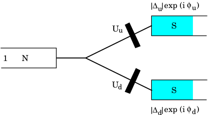
Figure 1: Schematic picture of the Andreev interferometer, consisting of a symmetric beam splitter with $\delta$-barriers added on the two arms where the superconducting leads are connected. The strength of the $\delta$-barriers can be varied in time, and are used as pumping fields.

The parameters to be varied in time are the strengths, $U_{\text{u}}$ and $U_{\text{d}}$, of two additional $\delta$-barriers placed in the two arms on the right side of Fig. 1. When all leads are in the normal state, the total scattering matrix $\mbox{\boldmath$S$}_{\text{N}}$ is obtained by combining the scattering matrix $\mbox{\boldmath$S$}_{\text{B}}$ given in Eq. (7) with the transmission and reflection amplitudes of the two $\delta$-barriers, namely

$$t=\frac{1}{1+i\beta_{\text{u/d}}}$$ (8)

and

$$r=-i\frac{\beta_{\text{u/d}}}{1+i\beta_{\text{u/d}}}$$ (9)

where $\beta_{\text{u/d}}=U_{\text{u/d}}/(\hbar v_{\text{F}})$, $v_{\text{F}}$ being the Fermi velocity. We choose as pumping fields $\beta_{\text{u/d}}$, i.e. the strength of the $\delta$-barriers. We consider the sinusoidal week pumping limit: $\beta_{\text{u}}=\bar{\beta}_{\text{u}}+\delta\beta_{\text{u}}\sin(\omega t)$ and $\beta_{\text{d}}=\bar{\beta}_{\text{d}}+\delta\beta_{\text{d}}\sin(\omega t-\delta\phi)$.

First we start by studying the case when the normal lead is tunnel-coupled to the rest of the structure, obtained by setting $\gamma\rightarrow 0$, $s_{1}=-1$ and $s_{2}=1$ in Eq. (7). The analytical expression for the charge pumped through lead 1, in leading order in $\gamma$, reads

$$Q_{1}^{\text{S}}=-A\frac{e}{\pi}\gamma^{2}4\sin(\Delta\Phi)\frac{\bar{\beta}_{\text{u}}^{2}+\bar{\beta}_{\text{d}}^{2}-2\bar{\beta}_{\text{u}}\bar{\beta}_{\text{d}}\cos(\Delta\Phi)}{\left[\left(\bar{\beta}_{\text{u}}+\bar{\beta}_{\text{d}}\right)^{2}+\cos^{2}\left(\frac{\Delta\Phi}{2}\right)\right]^{3}},$$ (10)

being $\Delta\Phi=\Phi_{\text{u}}-\Phi_{\text{d}}$ the phase difference, and $A=\pi\delta\beta_{\text{u}}\delta\beta_{\text{d}}\sin\delta\phi$ the area of the pumping cycle in parameter space. The $\gamma^{2}$ dependence of the charge in Eq. (10) is the expected one for transport mediated by Andreev reflection. It is interesting to note that $Q_{1}^{\text{S}}$ is an odd function of the phase difference, and that no pumping occurs at zero phase ($\Delta\Phi=0$). The pumped charge $Q_{1}^{\text{S}}$ can be contrasted with the linear DC conductance $G_{\text{DC}}=\frac{e^{2}}{h}2|\left(\mbox{\boldmath$\mathcal{R}$}_{\text{he}}\right)_{1,1}|^{2}$ of the system lambert_98 , with the barriers frozen at their average values $\bar{\beta}_{\text{u,d}}$, when a transport voltage is applied between the normal and the superconducting terminals (superconductors being at the same potential). For this particular case, in leading order in $\gamma$, $G_{\text{DC}}$ reads

$$G_{\text{DC}}=\frac{e^{2}}{h}\gamma^{2}\frac{1+4\left(\bar{\beta}_{\text{u}}^{2}+\bar{\beta}_{\text{d}}^{2}\right)+8\left(\bar{\beta}_{\text{u}}^{4}+\bar{\beta}_{\text{d}}^{4}\right)+(1+4\bar{\beta}_{\text{u}}^{2})(1+4\bar{\beta}_{\text{d}}^{2})\cos(\Delta\Phi)}{\left[\left(\bar{\beta}_{\text{u}}+\bar{\beta}_{\text{d}}\right)^{2}+\cos^{2}\left(\frac{\Delta\Phi}{2}\right)\right]^{2}}.$$ (11)

The DC conductance, Eq. (11), is an even function of the phase difference. It has a zero-phase extremum, which can be either a maximum or minimum depending on the strength of the barriers. To complete the analysis, we mention that the system acts as a pump also when all leads are in the normal state. To leading order the pumped charge is linear in $\gamma$ (as expected for vanishing superconducting gap), and it reads

$$Q_{1}^{\text{N}}=-A\frac{e}{\pi}4\gamma\frac{\bar{\beta}_{\text{u}}-\bar{\beta}_{\text{d}}}{\left[\left(\bar{\beta}_{\text{u}}+\bar{\beta}_{\text{d}}\right)^{2}+1\right]^{2}}\quad.$$ (12)

In contrast to the superconducting case, the leading order of the pumped charge vanishes when $\bar{\beta}_{\text{u}}=\bar{\beta}_{\text{d}}$.

Now, let us turn to the case of a maximally-transmitting beam splitter, which is obtained from Eq. (7) setting $\gamma=1/2$ and $s_{1,2}=1$. The analytical form for the charge pumped through lead 1 is rather involved and we report only the limits $\bar{\beta}_{\text{u/d}}\ll 1$ (large barrier transmission) and $\bar{\beta}_{\text{u/d}}\gg 1$ (small barrier transmission):

$$Q_{1}^{\text{S}}=\left\{\begin{array}[]{ll}\displaystyle 256A\frac{e}{\pi}\frac{(\bar{\beta}_{\text{u}}-\bar{\beta}_{\text{d}})\cos^{2}\left(\frac{\Delta\Phi}{2}\right)}{\left[3+\cos(\Delta\Phi)\right]^{3}}&\mbox{if}\quad\bar{\beta}_{\text{u/d}}\ll 1\\ \\ \displaystyle-A\frac{e}{\pi}\frac{\sin(\Delta\Phi)}{4\bar{\beta}_{\text{u}}^{3}\bar{\beta}_{\text{d}}^{3}}&\mbox{if}\quad\bar{\beta}_{\text{u/d}}\gg 1\end{array}\right..$$ (13)

It is interesting to note that while in the case of large barrier transmission $Q_{1}^{\text{S}}$ is an even function of the phase difference, for small transmission $Q_{1}^{\text{S}}$ is odd. However no definite parity is present for arbitrary transmissions $\bar{\beta}_{\text{u/d}}$ and, in particular, when $\bar{\beta}_{\text{d}}=0$ we obtain:

$$Q_{1}^{\text{S}}=\frac{128\bar{\beta}_{\text{u}}[1+(1+4{\bar{\beta}_{\text{u}}}^{2})\cos\Delta\phi-{\bar{\beta}_{\text{u}}}\sin\Delta\phi]}{[3+10{\bar{\beta}_{\text{u}}}^{2}+\cos\Delta\phi]^{3}}~{}.$$ (14)

Again, it is instructive to see what happens for the DC conductance, when the barriers are frozen to their average value. Also for this case, we report the same two limiting cases shown for $Q_{1}^{\text{S}}$

$$G_{\text{DC}}=\left\{\begin{array}[]{ll}\displaystyle\frac{e^{2}}{h}32\frac{\cos^{2}\left(\frac{\Delta\Phi}{2}\right)}{\left[3+\cos(\Delta\Phi)\right]^{2}}&\mbox{if}\quad\bar{\beta}_{\text{u/d}}\ll 1\\ \\ \displaystyle\frac{e^{2}}{h}\frac{\bar{\beta}_{\text{u}}^{4}+\bar{\beta}_{\text{d}}^{4}+2\bar{\beta}_{\text{u}}\bar{\beta}_{\text{d}}\cos(\Delta\Phi)}{8\bar{\beta}_{\text{u}}^{4}\bar{\beta}_{\text{d}}^{4}}&\mbox{if}\quad\bar{\beta}_{\text{u/d}}\gg 1\end{array}\right..$$ (15)

The DC conductance is an even function of the phase difference both large and small barrier transmission. It, actually, remains even also for arbitrary values of $\bar{\beta}_{\text{u/d}}$, while its zero-phase extremum can be either a maximum or a minimum depending on the values of $\bar{\beta}_{\text{u/d}}$. Finally, we report the pumped charge when the system is in the normal state

$$Q_{1}^{\text{N}}=\left\{\begin{array}[]{ll}\displaystyle-A\frac{e}{\pi}(\bar{\beta}_{\text{u}}-\bar{\beta}_{\text{d}})&\mbox{if}\quad\bar{\beta}_{\text{u/d}}\ll 1\\ \\ \displaystyle-A\frac{e}{\pi}\frac{1}{8\bar{\beta}_{\text{u}}^{2}\bar{\beta}_{\text{d}}^{2}}\left(\frac{1}{\bar{\beta}_{\text{u}}}-\frac{1}{\bar{\beta}_{\text{d}}}\right)&\mbox{if}\quad\bar{\beta}_{\text{u/d}}\gg 1\end{array}\right..$$ (16)

Contrasting Eq. (13) with Eq. (16), we notice that for the case $\bar{\beta}_{\text{u/d}}\ll 1$ , to leading order in the pumping parameters, superconductivity produces an enhancement of the charge pumped, reaching a maximum of a factor 4.

Finally, we wish to point out that the most distinctive signature of Andreev interference in the adiabatic pumping regime is the lack of a definite symmetry of the pumped current under inversion of the superconducting-phase difference. On the contrary, the DC current produced by an applied transport voltage, either DC or time-dependent, is always an even function of $\Delta\Phi$. The case of a DC voltage has been discussed above. It can be easily seen that also the current produced by rectification of an oscillating voltage $V_{\text{osc}}$ (for example induced by the pumping voltages on stray capacitances rectification ) is an even function of $\Delta\Phi$. In fact, the current produced by rectification reads rectification ; moskalets_01 $I_{\text{rect}}=\omega/2\pi\int_{0}^{2\pi/\omega}G(\tau)V_{\text{osc}}(\tau)d\tau$, where $G(\tau)$ is the instantaneous conductance which is an even function of $\Delta\Phi$, and all other quantities do not depend on the superconducting-phase difference. This lack of symmetry with respect to superconducting-phase difference can be exploited to distinguish between pumping and rectification. This is analogous to the normal case where the symmetry used for this purpose is the one related to magnetic field inversion rectification .

Conclusions. In this paper we have derived a scattering formula for adiabatically pumped charge in hybrid NS multi-terminal systems. This has been used to study Andreev interference in a 3-arm beam splitter attached to one normal and two superconducting leads with different phases of the order parameters. Within the weak pumping limit we found that Andreev interference very much affects the charge pumped through the normal lead, though differently with respect to the case of DC-voltage-driven transport. In general, the pumped charge has no definite symmetry under inversion of the superconducting-phase difference and no zero-phase extremum is found.

References

- (1) P. W. Brouwer, Phys. Rev. B 58, R10135 (1998).
- (2) F. Zhou, B. Spivak, and B. Altshuler, Phys. Rev. Lett. 82, 608 (1999).
- (3) M. Switkes, et al. Science 283, 1905 (1999).
- (4) Yu. Makhlin and A. D. Mirlin, Phys. Rev. Lett. 87, 276803 (2001).
- (5) L. S. Levitov, cond-mat/0103617 (2001).
- (6) O. Entin-Wohlman, A. Aharony, and Y. Levinson, Phys. Rev. B 65, 195411 (2002).
- (7) I.L. Aleiner, B.L. Altshuler and A. Kamenev, Phys. Rev. B 62, 10373 (2000).
- (8) M. Moskalets, and M. Büttiker, Phys. Rev. B 66, 035306 (2002).
- (9) M. Moskalets, and M. Büttiker, Phys. Rev. B 64, 201305 (2001).
- (10) E.R. Mucciolo, C. Chamon, and C.M. Marcus, Phys. Rev. Lett. 89, 146802 (2002).
- (11) M. Governale, F. Taddei, and R. Fazio, Phys. Rev. B 68, 155324 (2003).
- (12) S. K. Watson, R. M. Potok, C. M. Marcus, and V. Umansky, Phys. Rev. Lett. 91, 258301 (2003).
- (13) B. Wang, and J. Wang, Phys. Rev. B 65, 233315 (2002).
- (14) T. Aono, cond-mat/0311526 (2003).
- (15) R. Citro, N. Andrei, Q. Niu, Phys. Rev. B 68, 165312 (2003).
- (16) M. Blaauboer, Phys. Rev. B 68, 205316 (2003).
- (17) F. Zhou, cond-mat/9905190 (unpublished).
- (18) J. Wang, Y. Wei, B. Wang, and H. Guo, Appl. Phys. Lett. 79, 3977 (2001).
- (19) M. Blaauboer, Phys. Rev. B 65, 235318 (2002).
- (20) F. W. J. Hekking and Yu. V. Nazarov, Phys. Rev. Lett. 71, 1625 (1993).
- (21) V. C. Hui, and C. J. Lambert, Europhys. Lett. 23, 203 (1993)
- (22) Yu. V. Nazarov, Phys. Rev. Lett. 73, 1420 (1994).
- (23) A. V. Zaitsev, Phys. Lett. A 194, 315 (1994).
- (24) Yu. V. Nazarov and T. H. Stoof, Phys. Rev. Lett. 76, 823 (1996).
- (25) A. F. Volkov and A. V. Zaitsev, Phys. Rev. B. 53, 9267 (1996).
- (26) H. Nakano and H. Takayanagi, Solid State Comm. 80, 997 (1991).
- (27) S. Takagi, Solid State Comm. 81, 579 (1992).
- (28) C. J. Lambert, and R. Raimondi, J. Phys.: Condens. Matter 10, 901 (1998).
- (29) C.W.J. Beenakker, Phys. Rev. B 46, 12841 (1992).
- (30) S. Pilgram, H. Schomerus, A. M. Martin, and M. Büttiker, Phys. Rev. B 65, 045321 (2002).
- (31) P. W. Brouwer, Phys. Rev. B 63, 121303 (2001).
- (32) M. Moskalets and M. Büttiker, Phys. Rev. B 64, 201305(R) (2001).