Matter waves Degenerate Fermi gases

Collisions and expansion of an ultracold dilute Fermi gas

Abstract

We discuss the effects of collisions on the expansion of a degenerate normal Fermi gas, following the sudden removal of the confining trap. Using a Boltzmann equation approach, we calculate the time dependence of the aspect ratio and the entropy increase of the expanding atomic cloud taking into account the collisional effects due to the deformation of the distribution function in momentum space. We find that in dilute gases the aspect ratio does not deviate significantly from the predictions of ballistic expansion. Conversely, if the trap is sufficiently elongated the thermal broadening of the density distribution due to the entropy increase can be sizeable, revealing that even at zero temperature collisions are effective in a Fermi gas.

The expansion of an atomic gas following the sudden removal of the confining trap is known to provide valuable information on the state of the system and on the role of interactions [1]. In particular in the superfluid phase, where the macroscopic dynamics of the gas are governed by the equations of hydrodynamics, one expects anisotropic expansion if the gas is released from an anisotropic trap. This peculiar feature, which should be contrasted with the isotropic ballistic expansion exhibited by a non interacting gas, was first discussed in [2, 3] in the case of Bose gases and in [4] in the case of Fermi gases. Anisotropy is not however a unique feature exhibited by superfluids and also in the normal phase one can expect a similar behaviour if collisions are sufficiently important [3, 5, 6, 7]. This effect is expected to be particularly important in the case of Fermi gases interacting with large scattering lengths near a Feshbach resonance [8, 9, 10]. At first sight one would expect that the effects of collisions are suppressed at low temperature because of Pauli blocking. This is certainly true if one works close to equilibrium, as happens in the study of small amplitude oscillations [11]. In the problem of the expansion, however, large deformations in momentum space can be produced if one starts from a highly deformed cloud, with the result that collisions become effective even if the gas is initially at zero temperature. This interesting possibility was first pointed out in [12].

The aim of the present work is to calculate explicitly the dynamics of the expansion of a dilute, degenerate normal Fermi gas, taking into account the role of collisions. The main purpose is to provide quantitative predictions for the aspect ratio and the thermal broadening of the density distribution, as a function of the relevant parameters like the ratio of the trap frequencies, the scattering length and the number of atoms.

The system we consider is a dilute two component Fermi gas. At low temperatures the collisions between two atoms of the same species are suppressed due to Pauli blocking, and only atoms of different species can collide. We assume that the two species have the same mass and density. The starting point is the Boltzmann equation

$$\frac{\partial f}{\partial t}+{\bf v}_{1}\cdot\nabla_{\bf r}f-\frac{1}{m}\nabla U_{\rm ext}\cdot\nabla_{{\bf v}_{1}}f=C[f],$$ (1)

where for each component $f({\bf r},{\bf v}_{1},t)$ is the distribution function in phase-space and $U_{\rm ext}({\bf r})=(m/2)(\omega_{\perp}^{2}(x^{2}+y^{2})+\omega_{z}^{2}z^{2})$ is the external trap potential. We note that the potential is cylindrically symmetric, which is the form favoured by experiments. Moreover, in (1) we have neglected the mean field interaction term [13] which, however, has a minor effect on the expansion of a dilute Fermi gas [4]. The collisional integral in the case of a dilute Fermi system reads

$$C[f]=\frac{\sigma m^{3}}{4\pi h^{3}}\int d^{3}v_{2}\,d^{2}\Omega\,|{\bf v}_{1}-{\bf v}_{2}|[(1-f({\bf v}_{1}))(1-f({\bf v}_{2}))f({\bf v}^{\prime}_{1})f({\bf v}^{\prime}_{2})$$

$$-f({\bf v}_{1})f({\bf v}_{2})(1-f({\bf v}^{\prime}_{1}))(1-f({\bf v}^{\prime}_{2}))],$$ (2)

where in the low-energy limit, $\sigma=4\pi a^{2}$, with $a$ the s-wave scattering length. The scattering length is assumed to be smaller than the average distance between atoms.

The dynamics can be studied analytically using the method of the averages [14, 15] which involves calculating moments of the type $\langle\chi\rangle(t)=\int\chi({\bf r},{\bf v})f({\bf r},{\bf v},t)\,d^{3}r\,d^{3}v/\int f({\bf r},{\bf v},t)\,d^{3}r\,d^{3}v$. Applying this to (1) gives a set of equations of the general form

$$\frac{d\langle\chi\rangle}{dt}-\langle{\bf v}\cdot\nabla_{\bf r}\chi\rangle-\frac{1}{m}\langle\nabla U_{\rm ext}\cdot\nabla_{\bf v}\chi\rangle=\langle\chi C[f]/f\rangle,$$ (3)

where $\chi$ is a general function which depends on ${\bf r}$ and ${\bf v}$. Here we shall take moments of the form $\langle r_{i}^{2}\rangle$ , $\langle r_{i}v_{i}\rangle$ and $\langle(v_{i}-u_{i})^{2}\rangle$, where $u_{i}({\bf r})$ represents the velocity fields within the gas. If $\chi$ is a conserved quantity during a collision (i.e. $\Delta\chi=\chi_{1}+\chi_{2}-\chi_{1^{\prime}}-\chi_{2^{\prime}}$ is zero) then the collisional term disappears. This is true for the moments $\langle r_{i}^{2}\rangle$ and $\langle r_{i}v_{i}\rangle$ as well as for the quantity $\sum_{i}\langle(v_{i}-u_{i})^{2}\rangle$. This method has been used to study collective excitations in [11].

To explicitly include the collisional term in the calculations, it is convenient to introduce the following parametrization for the distribution function

$$f({\bf r},{\bf v},t)=\left[\exp\left(\frac{E({\bf r},{\bf v},t)-\mu}{T}\right)+1\right]^{-1},$$ (4)

with

$$E({\bf r},{\bf v},t)=\frac{m}{2}\sum_{i}\left[\frac{\omega_{i}^{2}r_{i}^{2}}{b_{i}^{2}}+\frac{(v_{i}-u_{i})^{2}}{K_{i}}\right],$$ (5)

where $u_{i}=\beta_{i}r_{i}$, and $\beta_{i}$, $b_{i}$, $K_{i}$, $\mu$ and $T$ are time dependent parameters, with $i\in\{x,y,z\}$. The ansatz (4,5) contains more free parameters than necessary, so that we can, without any loss of generality, set $\prod_{i}b_{i}=(\prod_{i}K_{i})^{-1/2}$. This fixes a unique definition of the effective temperature $T$ [16]. The chemical potential, $\mu$, is then obtained from the normalization condition, $(T/\hbar\bar{\omega})^{3}f_{3}({\rm e}^{\mu/T})=N/2$, where $N$ is the total number of atoms in both components, $\bar{\omega}^{3}=\prod_{i}\omega_{i}$, and $f_{s}(z)=\sum_{n}(-1)^{n+1}z^{n}/n^{s}$. From Eqs.(4,5) one can evaluate the entropy per particle of the gas, $S=(4\rho-\mu)/T$, where $\rho=Tf_{4}({\rm e}^{\mu/T})/f_{3}({\rm e}^{\mu/T})$. This result, taken together with the normalization condition, shows that there is a one-to-one correspondence between the entropy and the temperature $T$, and consequently changes in $T$ taking place during the expansion are associated with a change of entropy.

The ansatz (4,5) includes the initial equilibrium configuration predicted by Fermi statistics, and accounts for rescaling effects in coordinate as well as in momentum space. It allows, in particular, for anisotropic effects in momentum space which are crucial for describing correctly the mechanism of the expansion. The parametrization can describe both the collisionless and the hydrodynamic expansion as well as other intermediate regimes. Furthermore it accounts for possible changes in the effective temperature of the system during the expansion.

The next step is to evaluate the moments $\langle\chi\rangle$ in terms of the scaling parameters, which gives $\langle r_{i}^{2}\rangle=b_{i}^{2}\rho/m\omega_{i}^{2}$. Other moments can be expressed in terms of this quantity, so that $\langle r_{i}v_{i}\rangle=\beta_{i}\langle r_{i}^{2}\rangle$, $\langle(v_{i}-u_{i})^{2}\rangle=\omega_{i}^{2}K_{i}\langle r_{i}^{2}\rangle/b_{i}^{2}$, and $\langle u_{i}^{2}\rangle=\beta_{i}^{2}\langle r_{i}^{2}\rangle$. The moment equations then become

$$\beta_{i}=\frac{\dot{b}_{i}}{b_{i}}+\frac{\dot{\rho}}{2\rho},$$ (6)

$$\dot{\beta}_{i}+\beta_{i}^{2}-\frac{\omega_{i}^{2}}{b_{i}^{2}}K_{i}+\omega_{i}^{2}=0,$$ (7)

$$\frac{\dot{K}_{i}}{K_{i}}-2\frac{\dot{b}_{i}}{b_{i}}+4\beta_{i}=\frac{\langle(v_{i}-u_{i})^{2}C/f\rangle}{\langle(v_{i}-u_{i})^{2}\rangle},$$ (8)

where the final term in (7) arises from the confining potential. We set this term to zero in studying the expansion of the gas, while rescaling time in units of $\omega_{\perp}$, the original radial trap frequency. In addition, it is convenient to rewrite (8) as equations for the anisotropy in momentum space, $s=(K_{z}/K_{\perp})^{1/2}$, and the entropy, $S$

$$\frac{\dot{s}}{s}=\frac{\dot{b}_{\perp}}{b_{\perp}}-\frac{\dot{b}_{z}}{b_{z}}-\frac{(2+s^{2})}{4s^{2}}K^{2}\xi J(s,\tau),$$ (9)

$$\frac{T}{\rho}\dot{S}+\frac{(1-s^{2})}{2s^{2}}K^{2}\xi J(s,\tau)=0.$$ (10)

where we have defined

$$\frac{1}{\omega_{\perp}}\frac{\langle(v_{\perp}-u_{\perp})^{2}C/f\rangle}{\langle(v_{\perp}-u_{\perp})^{2}\rangle}=K^{2}\xi J\left(s,\tau\right),$$ (11)

with $J(s,\tau)$ given by

$$J(s,\tau)=\frac{3^{1/3}}{4\pi^{6}}\tau^{2}\frac{s^{5/3}}{f_{4}({\rm e}^{\mu/T})}\int d^{3}R\,d^{3}V_{1}\,d^{3}V_{2}\,d^{2}\Omega\,V^{\prime}\Delta V_{z}^{2}f({\bf V}_{1})f({\bf V}_{2})(1-f({\bf V}^{\prime}_{1}))(1-f({\bf V}^{\prime}_{2})).$$ (12)

Here $V^{\prime}=\sqrt{(V_{1x}-V_{2x})^{2}+(V_{1y}-V_{2y})^{2}+s^{2}(V_{1z}-V_{2z})^{2}}$, and we have rescaled variables so that $f({\bf V})=[\exp(R^{2}+V^{2}-\mu/T)+1]^{-1}$. The function $J$ depends on both $s$ and the reduced temperature $\tau=T/T_{F}$, where $T_{F}=(3N)^{1/3}\hbar\bar{\omega}$ is the Fermi temperature. In Eqs. (9-11) we have introduced the relevant dimensionless interaction parameter

$$\xi=(\lambda N)^{1/3}(k_{F}a)^{2},$$ (13)

where $k_{F}$ is the initial Fermi wavevector at the center of the trap, and $\lambda=\omega_{z}/\omega_{\perp}$ is the trap anisotropy. Further, we have introduced the geometric average $K=(K_{\perp}^{2}K_{z})^{1/3}=(b_{\perp}^{2}b_{z})^{-2/3}$.

Eq. (10) explicitly shows that the entropy (and hence the temperature) of the gas will remain constant during the expansion ($\dot{S}=0$) either in the absence of collisions ($J=0$) or when the distribution in momentum space is isotropic ($s=1$) [17]. The latter situation arises when starting from a spherical trap, $\lambda=1$, or when collisions are sufficiently frequent so that the gas is in the hydrodynamic regime. In regimes intermediate between the collisionless and hydroynamic limits, deformations in momentum space produce an increase of entropy and temperature. The equations (6-12) can also be used to study small oscillations around equilibrium, where the momentum distribution is isotropic ($s=1$). This procedure reproduces exactly the results of [11], in particular the collisional term takes the form $\langle(v_{i}-u_{i})^{2}C/f\rangle/\langle(v_{i}-u_{i})^{2}\rangle=(s-1)/\tilde{\tau}$, with $1/(\omega_{\perp}\tilde{\tau})=\mathcal{C}K^{2}\xi F_{Q}(T/T_{F})$ and $\mathcal{C}=8/(5\cdot 3^{5/3})$. Here $\tilde{\tau}$ is the typical relaxation time for the shape oscillations and $F_{Q}$ is given in [11]. Note that $1/\tilde{\tau}\propto T^{2}$ at small temperatures, so that the collisional contribution disappears when $T=0$. This is the result of Pauli blocking of collisions for a spherical momentum distribution. However, during expansion large deformations in momentum space can lead to collisions that scatter atoms outside of the Fermi surface, and the function $J$ differs from zero, even at zero temperature, as pointed out in [12].

We will assume that the gas is initially in equilibrium at low temperature, and that the effective temperature contained in the ansatz (4) remains small during the expansion. One can then expand the Fermi functions $f_{s}(z)$ using low-$T$ Sommerfeld expansions, so that the normalization condition gives $\mu\simeq T_{F}(1-\pi^{2}\tau^{2}/3)$, $\rho\simeq T_{F}(1+2\pi^{2}\tau^{2}/3)/4$ and $S=\pi^{2}\tau$. Substituting these expressions into (6,7,9,10) yields a new set of equations that can be solved numerically to study the time evolution of the gas. To simplify matters we also approximate the function $J(s,\tau)$ with its zero temperature value

$$J(s,0)=\frac{2\cdot 3^{4/3}s^{5/3}}{\pi^{6}}\int d^{3}R\,d^{3}V_{1}\,d^{3}V_{2}\,d^{2}\Omega\,V^{\prime}\Delta V_{z}^{2}\theta_{0}({\bf V}_{1})\theta_{0}({\bf V}_{2})(1-\theta_{0}({\bf V}^{\prime}_{1}))(1-\theta_{0}({\bf V}^{\prime}_{2})),$$ (14)

where we have rescaled the coordinates again such that $\theta_{0}({\bf V})=\Theta(1-V^{2}-R^{2})$, where $\Theta$ is the Heaviside step function. The integral for $J(s)$ can be evaluated numerically using a standard Monte Carlo technique, and is plotted in Fig. 1. Also plotted is the result $J(s)=2s^{8/3}/(3^{5/3}\pi)$ holding for large $s$, where the integral can be evaluated analytically by noting that virtually all collisions in this limit will scatter atoms outside of the Fermi surface (i.e. $(1-\theta_{0}({\bf V}^{\prime}_{1}))(1-\theta_{0}({\bf V}^{\prime}_{2}))\simeq 1)$. We shall discuss the validity of this zero-temperature approximation later.

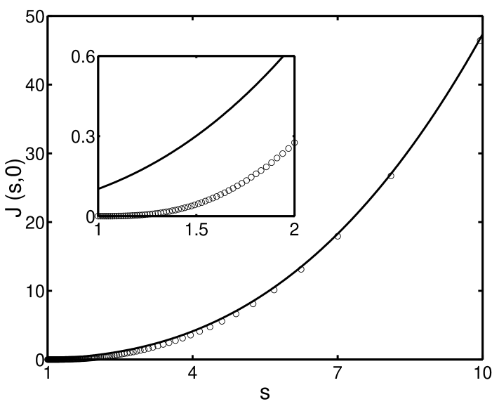
Figure 1: $J(s,0)$ as a function of $s$ for a range between $1$ and $10$, and (inset) between $1$ and $2$. The solid line shows the analytical form $J(s)=2s^{8/3}/(3^{5/3}\pi)$ for the limit $s\rightarrow\infty$.

We now use these equations to study the expansion for different choices of the trap anisotropies, $\lambda<1$, starting from a $T=0$ configuration [18]. We plot the aspect ratio of the cloud $\sqrt{\langle r_{\perp}^{2}\rangle/\langle z^{2}\rangle}=\lambda b_{\perp}/b_{z}$ as a function of time for $\xi=1$ and $\xi=20$ and compare to the expected collisionless and hydrodynamic behavior in Fig. 2. One notices that the effects of collisions are far less pronounced for $\lambda=0.3$, where the results are barely distinguishable from the collisionless behavior. However, for $\lambda=0.03$ the expansion lies intermediate between the two limits if one chooses $\xi=20$. This is to be expected since the deformation in momentum space reached in this case is much larger. In particular, in the collisionless case one would expect $s\rightarrow 1/\lambda$ at long times, and this fixes the maximum $s$ possible. Since $J$ takes large values only for large $s$, then the collisional term is potentially more effective for smaller $\lambda$.

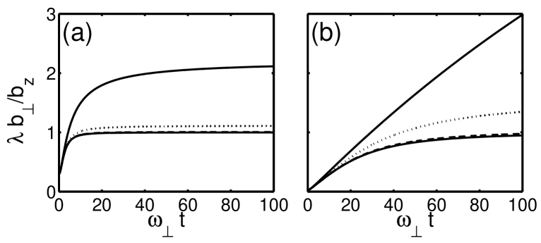
Figure 2: Aspect ratio against time for the free expansion of a zero-temperature Fermi gas from a trap with (a) $\lambda=0.3$ and (b) $\lambda=0.03$. The upper and lower solid lines on each plot represents the behavior in the hydrodynamic and collisionless regimes respectively, with the other lines displaying results of solving the equations (6-12) for $\xi=1$ (dashed) and $\xi=20$ (dotted).

An interesting consequence of the momentum space deformation is that atoms scattering outside the Fermi surface will tend to smooth out the distribution function. This aspect appears in (10) as an increase in the temperature, even if we start from an initial $T=0$ configuration. Fig. 3(a) shows the temperature calculated at $\omega_{\perp}t=100$ for different values of $\lambda$. Again, one sees a much larger effect for $\lambda\ll 1$. The function tends to zero for both $\xi\rightarrow 0$ and $\xi\rightarrow\infty$, representing the crossover from collisionless to hydrodynamic behavior in a similar manner to damping times in collective oscillations [11, 14]. Since (10) is an equation for $\tau^{2}$ one finds that starting from a non-zero temperature, $\tau_{0}$, gives a final temperature of approximately $\tau=\sqrt{\tau_{0}^{2}+(\delta\tau)^{2}}$, where $\delta\tau$ is the change for an initially zero temperature gas obtained from Fig. 3(a). Hence the temperature increase produced by collisions will become smaller as one raises the initial temperature of the gas.

The change in temperature during the expansion, as well as the fact that experiments will be initially at a non-zero temperature, will lead to corrections to the zero-temperature collisional term (14). We can estimate the effects at finite temperatures by approximating $J(s,\tau)$ (12) with the sum of the zero-$T$ result to that derived for finite-$T$ but small deformations, so that $J(s,\tau)=J(s,0)+\mathcal{C}(s-1)F_{Q}(\tau)$, with the function $F_{Q}(\tau)$ given in [11]. We find that the inclusion of the temperature dependence in $J$ has little impact on the results, even allowing for an initial temperature of $\tau=0.2$.

Since for a dilute gases ($k_{F}|a|\ll 1$) the value of $\xi$ for realistic parameters will be, at most, of the order of 1, we conclude that collisional effects on the aspect ratio of the expanding gas are negligible (see Fig. 2). This is consistent with experimental results in dilute degenerate gases (see for example [9, 19]). In contrast, we find that the effect of collisions on the thermal broadening can be significant at low temperatures even if $\xi\simeq 1$, especially for highly deformed traps. As an example in Fig. 3(b) we show the column density $n(r_{\perp})=(m/h)^{3}\int dzd{\bf v}f({\bf r},{\bf v},t)$, calculated at $\omega_{\perp}t=100$, $\lambda=0.03$ and $\xi=1$, starting from an initial zero temperature configuration. Around $80\%$ of the increase in $T$ (and the consequent broadening of the density profile) takes place over the first $\omega_{\perp}t=20$ of the expansion. The comparison with the prediction of ballistic expansion (dashed line) explicitly reveals the importance of collisions. Experimentally one could observe this difference by cooling down a two component Fermi gas to very low temperatures. Ballistic expansion could be achieved either by first removing one of the two components, or by suddenly tuning the scattering length to zero at the start of the expansion.

In order to also observe large effects in the aspect ratio one should increase the value of $\xi$, and hence of $k_{F}|a|$, by, for example working close to a Feshbach resonance. In this case, however, the formalism of the Bolzmann equation is not strictly applicable. A rough estimate of the collisional effects can be obtained by replacing $a^{2}$ with the unitarity limited expression $a^{2}/(1+K(k_{F}a)^{2})$, where $k_{F}$ is the initial Fermi momentum and $K$ accounts for the decrease of the density during the expansion. In the unitarity limit $k_{F}|a|\rightarrow\infty$ equation (11) is then modified by replacing $K^{2}$ with $K$ and setting $\xi=(\lambda N)^{1/3}$. These changes result in a sizable increase of the anisotropy effects. Apart from the fact that the parameter $\xi$ can easily take large values, the replacement of $K^{2}$ with $K$ makes the collisional term effective for longer times during the expansion. One should however note that in the unitarity limit the gas is expected to be superfluid at low temperatures and its dynamics should be consequently described by the hydrodynamic equations of superfluids.

In conclusion we have shown that collisions can be effective in a dilute normal Fermi gas even at zero temperature, as a consequence of large deformations of the distribution function in momentum space after expansion from a very elongated trap. They can give rise to a sizeable entropy increase and hence thermal broadening of the density distribution, which should be visible by imaging the atomic cloud. In contrast a $T=0$ superfluid should expand anisotropically, without any entropy increase due to the absence of collisions.

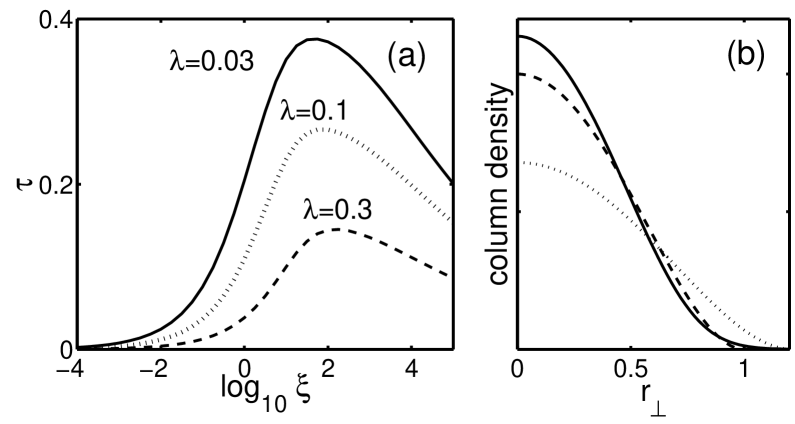
Figure 3: (a) Temperature at $\omega_{\perp}t=100$, $\tau=T/T_{F}$, as a function of $\xi$, for different values of $\lambda$. The gas prior to expansion is at zero temperature.(b) Column density (see text) as a function of radial distance at $\omega_{\perp}t=100$, for $\lambda=0.03$ and $\xi=1$ (solid line), compared to the result of expansion in the collisionless (dashed) and hydrodynamic (dotted) limits. Both axes are in arbitrary units.

- [1] \NameDalfovo F., Giorgini S., Pitaevskii L. P. Stringari S. \REVIEWRev. Mod. Phys.711999463.
- [2] \NameCastin Y. Dum R. \REVIEWPhys. Rev. Lett.7719965315.
- [3] \NameKagan Yu., Surkov E. L. Shlyapnikov G. V. \REVIEWPhys. Rev. A551997R18.
- [4] \NameMenotti C., Pedri P. Stringari S. \REVIEWPhys. Rev. Lett.892002250402.
- [5] \NameWu H. Arimondo E. \REVIEWEurophys. Lett.431998141.
- [6] \NameSvarchuck I. et al. \REVIEWPhys. Rev. A682003063603.
- [7] \NameGerbier F. et al. \REVIEWPhys. Rev. Lett.922004030405.
- [8] \NameO’Hara K. M. et al. \REVIEWScience29820022179.
- [9] \NameRegal C. A. Jin D. S. \REVIEWPhys. Rev. Lett.902003230404.
- [10] \NameBourdel T. et al. \REVIEWPhys. Rev. Lett.912003020402.
- [11] \NameVichi L. \REVIEWJ. Low Temp. Phys.1212000177.
- [12] \NameGupta S. et al. \REVIEWPhys. Rev. Lett.922004100401.
- [13] \NameGuéry-Odelin D. \REVIEWPhys. Rev. A662002033613.
- [14] \NameGuéry-Odelin D. et al. \REVIEWPhys. Rev. A6019994851.
- [15] \NamePedri P., Guéry-Odelin D. Stringari S. \REVIEWPhys. Rev. A682003043608.
- [16] Alternatively, one can fix the value of to the initial value and obtain an equivalent set of equations, as in the work of Pedri et al.[15]. The choice made in the present work is particularly convenient if the expansion starts from a configuration.
- [17] Note that Eq. (10) can also be obtained by starting strictly from the Boltzmann H-theorem.
- [18] In practice, the approximation is compatible with the assumption that the gas is non superfluid, the critical temperature for the BCS transition being exponentially small in a dilute gas.
- [19] \NameDeMarco B. Jin D. S. \REVIEWScience28519991703.