Critical dynamics of the Potts model: short-time Monte Carlo simulations.

Abstract

We calculate the new dinamic exponent $\theta$ of the 4-state Potts model, using short-time simulations. Our estimates $\theta_{1}=-0.0471(33)$ and $\theta_{2}=$ $-0.0429(11)$ obtained by following the behavior of the magnetization or measuring the evolution of the time correlation function of the magnetization corroborate the conjecture by Okano et. al. In addition, these values agree with previous estimate of the same dynamic exponent  for the two-dimensional Ising model with three-spin interactions in one direction, that is known to belong to the same universality class as the 4-state Potts model. The anomalous dimension of initial magnetization $x_{0}=z\theta+\beta/\nu$ is calculated by an alternative way that mixes two different initial conditions. We have also estimated the values of the static exponents $\beta$ and $\nu$. They are in complete agreement with the pertinent results of the literature.

PACS: 05.50.+q, 05.10.Ln, 05.70.Fh

I Introduction

Several results about critical phenomena have been recently obtained using Monte Carlo simulations in short-time regime Zheng . Such simulations are more convenient than traditional ones done in the equilibrium regime because they circumvent a known problem in computational physics: the critical slowing down phenomena.

Investigating Monte Carlo simulations before attaining equilibrium permits to us obtaining the static critical exponents ($\beta$ and $\nu$) but also leads to the less known dynamical ones. The scaling equation for non-equilibrium regime was obtained by Jansen et al. Jansen , on the basis of renormalization group theory. For systems without conserved quantities like energy and magnetization (model A in the terminology of Halperin and Hohenberg Halperin ), it is written as

$$M^{(k)}(t,\tau,L,m_{0})=b^{\frac{-k\beta}{\nu}}M^{(k)}(b^{-z}t,b^{\frac{1}{\nu}}\tau,b^{-1}L,b^{x_{0}}m_{0})$$ (1)

where $m_{0}$ is the initial magnetization, $x_{0}=$ $x_{0}(m_{0})$ PRL do Zheng is the anomalous dimension of the initial magnetization, $\beta$ and $\nu$ are the known static exponents and $z$ is the dynamic one ($\tau\sim\xi^{z}$). The values of $M^{(k)}$ are the $k$th moments of magnetization, defined by $M^{(k)}=\left\langle M^{k}\right\rangle$, where $\left\langle\cdot\right\rangle$ indicates an average over several samples randomly initialized but satisfying the condition of having the same magnetization $(m_{0})$ at the beggining. The relevance of this result is allowing to include the dependence on the initial conditions of the dynamic systems in their non-equilibriun relaxation. As an important consequence, they could advance the existence of a new critical exponent $\theta$, which is independent of the known set of static exponents and even of the dynamic exponent $z$.

By considering large systems and choosing $\tau=0$ $(T=T_{c})$ ; $b^{-z}t=1$ in the equation (1), we obtain the dynamic scaling law for the magnetization:

$$M(t,m_{0})=t^{\frac{-\beta}{\nu z}}M(1,t^{\frac{x_{0}}{z}}m_{0}).$$ (2)

Expanding $M$ around the zero value of the parameter $u=t^{\frac{x_{0}}{z}}m_{0}$, one obtains:

$$M(t,m_{0})=m_{0}t^{\theta}+O(u^{2})$$ (3)

which leads to the power law:

$$M(t)\sim m_{0}t^{\theta}$$ (4)

whereas $t<t_{0}\sim m_{0}^{-\frac{z}{x_{0}}}$ since in this regime $u\ll 1$. This new universal stage, characterized by the exponent $\theta=\left(x_{0}-\frac{\beta}{\nu}\right)/z$ , has been exhaustively investigated to confirm theoretical predictions and to enlarge our knowledge on phase transitions and critical phenomena.

Indeed the anomalous behavior of the magnetization at the beginning of relaxation, also called critical initial slip, was originally associated to a positive value of $\theta$. This kind of behavior was confirmed in the kinetic $q=2$ and $3-$state Potts models Zheng , as well as in irreversible models like the majority voter one TTome and the probabilistic cellular automaton proposed by Tomé and Drugowich de Felício to describe part of the immunological system TD . However, the exponent $\theta$ can also be negative. This possibility was observed in the Blume-Capel model (analytical oerding and numerically nossopaperphysrevE ) and in the Baxter-Wu model (numerically Drugoarashiro ), an exactly solvable model which shares with the $4-$state Potts model the same set of critical exponents. In addition, a negative but close to zero value for $\theta$ was obtained for the two-dimensional  (2-D) Ising model with three-spin interactions in just one direction (IMTSI) DrugoSimoes , a model which is also known to behave to the $4-$state Potts model universality class.

However, at the best of our knowledge a numerical determination of the exponent $\theta$ for this special case ($q=4$) of the Potts model continues to be lacking. Thus, we decided to investigate the short-time behavior of that model in order to better understand its dynamics and also to learn about the role of the exponent $x_{0}$ of the nonequilibrium magnetization concerning the well established classification of the models (at least in what concerns the static behavior) in the universality classes.

As we mentioned above the estimates for the exponent $\ \theta$ for two models that belong to the same universality class as the 4-state Potts model have revealed discrepant results. Whereas the two-dimensional Ising model with threee spin interactions in one direction (IMTSI) obeys the conjecture by Okano et al. Okano ($\theta$ should be negative and close to zero) DrugoSimoes the Baxter-Wu model Drugoarashiro strongly disagrees from that prediction. Putting in numerical values, whereas the IMTSI model exhibits a small and negative value $(-0.03\pm 0.01)$ for $\theta$, when studying the BW model we found $\theta=-0.186\pm 0.002$.

In this paper we study the short-time behavior of the two-dimensional four-state Potts model and present numerical estimates for $\theta$ using two different methods. First, we fix the initial value of the magnetization and follow its time evolution to obtain $\theta(m_{0})$ which in turn can be extrapolated to lead to $\theta$ when $m_{0}\rightarrow 0$. Second, we deal with the time correlation of the magnetization defined by TTome :

$$C(t)=\frac{1}{N^{2}}\left\langle M(t)M(0)\right\rangle$$ (5)

where the average is done over samples whose initial magnetizations are randomly choosen but obey $\left\langle M(0)\right\rangle=0$. In reference TTome it was shown that this quantity exhibits at $T=T_{c}$ the power-law behavior:

$$C(t)\sim t^{\theta}\text{.}$$ (6)

This approach has several advantages when compared to the other technique but its application was initially restricted to the models which exhibit up-down symmetry. Recently, Tome TTomeII has shown that this result is more general and can be applied whenever the model presents any group of symmetry operations related to the Markovian dynamics. Equation 6 was shown to be valid for instance in the antiferromagnet ordering model, models with one absorvent state and even in the Baxter-Wu model Drugoarashiro which exhibits a $Z(2)\otimes Z(2)$ symmetry.

It is well known that the $q\neq 2$ Potts Model does not have up-down symmetry. However, based on the paper of Tomé TTomeII we can use this approach to calculate the exponent $\theta$ of the three- and four-state Potts models.

We checked this possibility working with the three-state Potts model. Our estimate is $\theta=0.072(1)$, in good agreement with the result obtained by Zheng Zheng ($\theta=0.070(2)$) and with the estimate obtained by Brunstein and Tome Brunstein using a cellular automaton which exhibits C3v symmetry, the same as the three-state Potts model. A plot of the correlation function of the magnetization $C(t)$ in this case is presented in the Fig. 1.

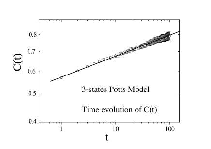
Figure 1: Log-log plot of $C(t)\times t$ to 3-states Potts Model

In the sequence we estimated the exponent $\theta$ of the 4-state Potts model which agrees with the conjectured by Okano et al. In addition, they agree with previous estimates for $\theta$ obtained by Simões and Drugowich de Felício DrugoSimoes .

To confirm our first estimate we simulated the magnetization evolution for four different initial values of $m_{0}$ which after extrapolated ($m_{0}\rightarrow 0$) led to a similar result.

It is clear that having the exponent $\theta$ the anomalous dimension $x_{0}$ follows. But inspired in previous studies nosso paper Phys. Letters we decided to investigate a direct manner in determining $x_{0}$ using mixed initial conditions. In order to build the adequate function we remember that when in contact with a heat bath at $T=T_{c}$ the magnetization of completely ordered samples ($m_{0}=1$) decays like a power law

$$M(t)\sim t^{{}^{\frac{-\beta}{\nu z}}}\text{.}$$ (7)

Thus, according to the scaling relations (4) and (7) it is enough to work with the ratio

$$F_{3}(t,L)=\frac{\left\langle M\right\rangle_{m_{0}\rightarrow 0}}{\left\langle M\right\rangle_{m_{0}=1}}$$ (8)

to obtain a power law which decays as $t^{\theta+\beta/\nu z}$ $=t^{x_{0}/z}$ . Using $z$ as input nosso paper Phys. Letters we can achieve the value of $x_{0}$. On the other hand, by following the relation (7) we estimate the ratio $\beta/\nu z$ which can be compared with the exact result $\beta/\nu=1/12$ after using the value of the dynamical exponent $z$.

Finally using derivatives of the magnetization at an early time and once more the value of $z$ as input we obtain the critical exponent $\nu$ of the correlation length, whose numerical estimates by usual techniques (phenomenological renormalization group, hamiltonian studies and equlibrium Monte Carlo simulations) are always very different from the pertinent result ($\nu=2/3$).

The paper is organized as follows: in the next section we present a brief review and some details of the simulation. The results are presented in Section 3 and our conclusions are in section 4.

II The kinetic $4$-states Potts model

In time-dependent simulations we are interested in finding power laws for physical quantities even when the system is far from equilibrium. In this regimen the magnetization $M(t)$ must be calculated as an average over several samples because the system does not obey any a priori probability distribution. The average can be done in different ways: we can prepare all the samples with the same initial magnetization (sharp preparation) or generate samples which satisfy a less restrict criteria like to have mean value of the magnetization equal to zero.

The $q$ states Potts model ferromagnetic without the presence of an external field is defined by the Hamiltonian potts :

$$H=-J\sum\limits_{\left\langle i,j\right\rangle}\delta_{\sigma_{i},\sigma_{j}}$$ (9)

where $J$ denotes the interaction between the nearest neighbors $\left\langle i,j\right\rangle$ and $\sigma_{i}$ can assume different values $\sigma_{i}=0,1..,q-1$. If two spins are parallel they contribute with energy $-J$, else the energy is null.

The critical temperature of this model, is known exactly potts ,

$$\frac{J}{k_{B}T}=\log[1+\sqrt{q}].$$ (10)

The magnetization, different of other models as Ising and Blume Capel is not only the sum of variables of spin. A general expression used for the magnetization in the Potts model that considers an average over the sites and over the samples is written as

$$\left\langle M(t)\right\rangle=\frac{1}{N_{s}(q-1)N}\sum\limits_{j=1}^{N_{s}}\sum\limits_{i=1}^{L^{d}}(q\delta_{\sigma_{i,j}(t),1}-1)$$ (11)

where $\sigma_{i,j}$ denotes the spin $i$ of the $j$th. sample at the $t$th. MC sweep. Here $N_{s}$ denotes the number of the samples and $L^{d}$ is the volume of the system. This kind of simulation is performed $N_{B}$ times to obtain our final estimates as a function of $t$. In order to prepare a lattice with a given magnetization we need to choose the states $\sigma_{i}=0,1,2,3$ in each site with equal probability (1/4). Next we measure the magnetization and change states in sites randomly chosen in order to obtain a null value for the magnetization. Finally we change $\delta$ sites occupied by $\sigma_{i}=0,2$ or $3$ and substitute by $\sigma_{i}=1$. The initial magnetization in this case will be given by:

$$m_{0}=\frac{4\delta}{3N}$$ (12)

where $N=L^{d}$.

We have chosen to update the spins according to the heat bath algorithm, which means that the probability that the spin $\sigma_{\overrightarrow{x}}$ localized at the site $\overrightarrow{x}$ can assume another value $\sigma_{\overrightarrow{x}}^{f}$ is given by:

$$P(\sigma_{\overrightarrow{x}}\rightarrow\sigma_{\overrightarrow{x}}^{f})=\frac{\exp(-\frac{J}{k_{B}T}\sum\limits_{\overrightarrow{k}}\delta_{\sigma_{\overrightarrow{x}+\overrightarrow{k}}(t),\sigma_{\overrightarrow{x}}^{f}})}{\sum\limits_{\sigma_{\overrightarrow{x}}^{f}=0}^{3}\exp(-\frac{J}{k_{B}T}\sum\limits_{\overrightarrow{k}}\delta_{\sigma_{\overrightarrow{x}+\overrightarrow{k}}(t),\sigma_{\overrightarrow{x}}^{f}})}$$ (13)

where $\sum\limits_{\overrightarrow{k}}$ denotes the sum about the nearest neighbors sites of the spin at the site $\overrightarrow{x}$ .

III Results

We performed Monte Carlo simulations for $N_{B}=5$ different bins and four different initial magnetizations, $m_{0}=4\delta/3N\approx 0.033$, $0.049$, $0.066$ and $0.082$, for a lattice of size $L=90$. These magnetizations correspond respectively to $\delta=200$, $\delta=300$, $\delta=400$, $\delta=500$ according to the expression (12). To estimate the errors we ran $5$ different bins, with $35000$ samples each one.

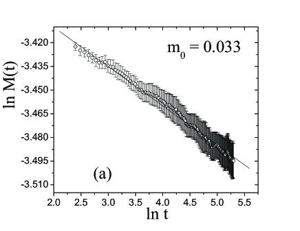
Figure 2: Time evolution of the magnetization for $m_{0}=0.033$.

In the figs. 2 and 3 we present the log-log plot for two different initial magnetizations and two different values of $m_{0}=0.033$ and $m_{0}=0.082$ respectively. The fit had excellent goodness $(Q=0.99)$ in the entire range $[t_{i},t_{f}]\subset[0,200]$. We have chosen the range $[10,100]$ to estimate the value to $\theta$ for all initial magnetizations. We must note that the slope is positive for $m_{0}=$ $0.082$  but changes the signal at some value between  $0.066$  and $0.049$. This trend to a negative value can be also certified in the Fig. 4 that shows the plot of $\theta=\theta(m_{0})$. It is worth to mention that there is a clear linearity in the plot of $\theta$ versus the initial magnetization (see fig. 4) but big fluctuations are observed in the evolution of the magnetization in each case.The value found for $\theta_{ext}$ is $-0.0471(33)$ is in fair agreement with the result DrugoSimoes for the IMTSI model and strongly disagrees with the result obtained for the Baxter-Wu model.

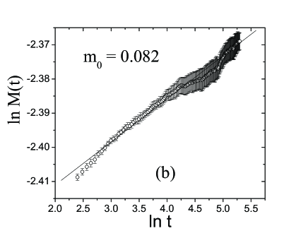
Figure 3: Time evolution of the magnetization for $m_{0}=0.082$.

We also ran Monte Carlo simulations to obtain the time-evolution correlation $C(t)$, and the the dynamic exponent $\theta$ according to the relation (6). For the same interval $[10,100]$ we have gotten the estimate $\theta=$ $-0.0429(11)$ that corroborates the above estimate $-0.0471(33)$ obtained from the evolution of the non-equilibrium magnetization. We used $35000$ samples and once more 5 different bins to make this estimate. In figure 5 it is shown the log-log plot of $C(t)\times t$ for the four-state Potts model.

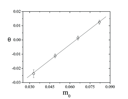
Figure 4: $\theta$ as function of $m_{0}$ in the 4-state Potts Model (extrapolation)

Equilibrium simulations for the four-state Potts model are ever acompannied by strong fluctuations. The reason is the presence in the Hamiltonian of a marginal operator characterized by an anomalous dimension equal to zero. If we hope some signal of that anomalous behavior in short-time simulations done far from equilibrium we should look for that in the only new anomalous dimension: that of the initial magnetization $x_{0}$. In order to confirm the null value for the anomalous dimension we estimate directly $x_{0}$ using the reported function $F_{3}$.

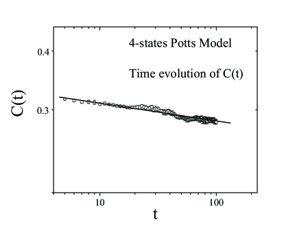
Figure 5: Log-log plot of $C(t)\times t$ to 4-states Potts Model

Over here we used $N_{b}=5$ bins for each initial condition and again the $N_{s}=35000$ realizations. A plot when the initial magnetization is $m_{0}=0.082$ can be seen in the fig. 6. Extrapolating    to $m_{0}\rightarrow 0$ we found $\left(x_{0}/z\right)_{ext}=0.0077(33)$ with the same set initial magnetizations $m_{0}$ that was used to extrapolating $m_{0}$. Using as input $z=2.290(3)$, we obtain $x_{0}=0.0176(75)$.

The value of $\beta/\nu$ can be obtained directly of magnetization decay of a initial ordered state, considering the relation:

$$\frac{\beta}{\nu}=\left(\frac{\beta}{\nu z}\right)_{c}\cdot z\text{.}$$ (14)

The value of the exponent obtained from the decay $(M\sim t^{-\frac{\beta}{\nu z}})$, was $\left(\frac{\beta}{\nu z}\right)_{c}=0.0547(1)$ with $Q=0.84$.

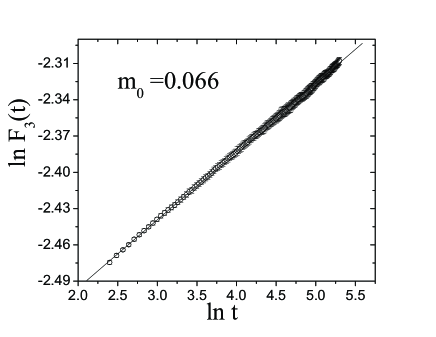
Figure 6: Plot of $F_{3}$ function for case $m_{0}=0.066.$

Using as the input the same value for $z$ value we achieved $\frac{\beta}{\nu}=0.12526(28)$ that is in a good agreement with the exact result $\frac{\beta}{\nu}=0.125$ potts .

Finally to find the exponent $\nu$, we calculated the expected decay of derivative

$$D(t)$$

   (15)

According to the reference (1), for $m_{0}=1$, we expect of $D(t)$ the power law behavior

$$D(t)\sim t^{\frac{1}{\nu z}}$$ (16)

and so $\nu=$ $\left(\dfrac{1}{\nu z}\right)_{c}^{-1}\dfrac{1}{z}$. In the Fig. 7 we illustrate the power law (16), performing simulations with $N_{s}=8000$ samples with $N_{b}=5$ to estimate errors and $t_{\max}=1000$ MC steps.

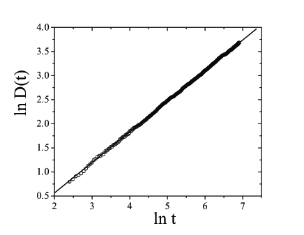
Figure 7: Time dependence of derivative $D(t)$ of the 4-state Potts Model. The slope gives $1/\nu z$.

Our best estimative is $\dfrac{1}{\nu z}=0.65453(46)$, in the interval $[10,1000]$ with $Q=0.99$. The value found to $\nu$ at this interval is $\nu=0.667(1)$. The value $\left(\dfrac{1}{\nu z}\right)_{c}$ also is used to estimate $\beta$. This minimizes the errors because:

$$\beta=\left(\frac{\beta}{\nu z}\right)_{c}\left(\dfrac{1}{\nu z}\right)_{c}^{-1}$$ (17)

The value found to $\beta$ is $0.0836(2).$ These  values are in complete agreement with conjectured results $\nu=2/3=0.\overline{6}$ and $\beta=1/12=0.08\overline{3}$.

IV Conclusions

We calculated the dynamic exponent $\theta$ of the four-state Potts Model using two different techniques: the time-evolution of the magnetization when the samples are prepared with a small and nonzero value of $m_{0}$ for four different values of initial magnetization and through of the time correlation of the magnetization. The values found for $\theta$ in both cases corroborate the conjecture by Okano et al. and are in complete agreement with the estimate obtained for another model which is in the same universality class as the 4-state Potts model: the 2-D Ising model with three-spin interactions in one direction. We also estimated directly the anomalous dimension of the initial magnetization $x_{0}$ which results very closed to zero. The same does not occur in the Baxter-Wu model that, although exhibiting the same leading exponents as the 4-state Potts model, does not own a marginal operator which prevents us from determine with good precision the critical exponents.

We also estimated the static exponents $\beta$ and $\nu$ using the short-time Monte Carlo simulations and our results are in surprisingly agreement with pertinent results.

As an additional contribution we present a new estimate for the exponent $\theta$ of the 3-state Potts Model working with the time evolution of the time correlation of the magnetization $C(t)$. This kind of approach has been previoulsy used by Brunstein and Tomé when studying a four-state cellular automaton with C-3$\nu$ symmetry Brunstein .The result agrees with estimates obtained from the evolution of the magnetization Zheng after the extrapolation ($m_{0}\rightarrow 0$).

References

- (1) B. Zheng, Int. J. Mod. Phys. B 12, 1419 (1998);
- (2) H. K. Janssen, B. Shaub and B. Schmitmann, Z, Phys. B 73, 539 (1989);
- (3) B. I. Halperin, P. C. Hohenberg and S- K. Ma, Phys. Rev. B 10, 139 (1974);
- (4) Z. B. Li, L. Schülke, B. Zheng, Phys. Rev. Lett. 74, 3396 (1995);
- (5) T. Tomé, M. J. de Oliveira, Phys. Rev. E 58, 4242 (1998).
- (6) T. Tomé and J. R. Drugowich de Felício, Phys. Rev. E 53, 108 (1996)
- (7) H. K. Janssen and K. Oerding, J. Phys. A: Math. Gen. 27, 715 (1994)
- (8) R. da Silva, N. A. Alves, J. R. Drugowich de Felício, Phys. Rev. E 66, 026130 (2002);
- (9) E. Arashiro, J. R. Drugowich de Felício, Phys. Rev. E 67, 046123 (2003);
- (10) C. S. Simões, J. R. Drugowich de Felício, Mod. Phys. Lett. B 15, 487 (2001);
- (11) K. Okano, L. Shülke, K. Yamagishi, B. Zheng, Nucl. Phys. B 485, 727 (1997);
- (12) T. Tomé, J. Phys. A-Math 36 (24): 6683 (2003)
- (13) A. Brunstein and T. Tomé, Phys. Rev. 60, 3666 (1999)
- (14) R. da Silva, N. A. Alves, J. R. Drugowich de Felício, Phys. Lett. A 298, 325 (2002);
- (15) F. Y. Wu, Rev. Mod. Phys 54, 235 (1992);