Local persistense and blocking in the two dimensional Blume-Capel Model

Abstract

In this letter we study the local persistence of the two–dimensional Blume– Capel Model by extension of the concept of Glauber dynamics. We verify that for any value of the ratio $\alpha=D/J$ between anisotropy $D$ and exchange $J$ the persistence shows a power law behavior. In particular for $\alpha<0$ we find a persistence exponent $\theta_{l}=0.2096(13)$, i.e. in the Ising universality class. For $\alpha>0$ ($\alpha\neq 1$) we observe the occurrence of blocking.

Among the many relevant quantities of interest in the modelling of nonequilibrium dynamics of spin systems such as first time passage Feller , which has been extensively discussed in the literature due to the appearance of non–trivial exponents in the power law behavior of the first return probability as function of time, another quantity of interest is that of persistence, i.e. the characterization of the time it takes for a particular spin not to change its state from its given $t=0$ configuration. Defining $P(t)$ as the probability that a particular spin will not flip up to time $t$, at zero temperature temperature and for the Ising and Potts models this quantity was shown to behave as B.Derrida ; Stauffer

$$P(t)\sim t^{-\theta_{l}},$$ (1)

where the persistence exponent $\theta_{l}$ describes the non-equilibrium relaxation of the system. This has been determined through coarsening simulations since one expects that the fraction of spins which do not change up to $t$ represents a good estimate of $P(t)$. As a consequence one may introduced a global version of the concept of persistence through the quantity $P_{g}(t)$ which represents the probability that the magnetization does not change its sign from its $t=0$ value, as done in S.N.Majundar . Recently one of the authors explored these ideas to determine the associated $\theta_{g}$ exponent in the Blume Capel Model, in particular its behavior at the critical and tricritical points blumeglobal . It was found that the exponent shows an abrupt change as one goes from the critical points ($\theta_{g}\simeq 0.23$, Ising universality class) to the tricritical one.

The purpose of this letter is to extend the Glauber dynamics to the Blume Capel Model and to study the influence of the anisotropy on the exponent $\theta_{l}$. For the sake of clarity, we start with a brief overview of the Ising model.

At $T=0$ the dynamics can be greatly affected by local blocking configurations, and the energy necessary to overcome them might be so high as to render the system static. On the other hand, for $T\neq 0$ it becomes difficult to define domains because one might not be able to distinguish between true domains and spin flips due to thermal fluctuations. Nonetheless for the Ising Model these difficulties can be overcome and a power law a power law decay for the fraction of persistent spins was ascertained in the whole low temperature phase Derrida . The calculated values of the exponent were $\theta_{l}=0.22$, $0.22$ and $0.29$ for $T=0$, $T=T_{c}/3$ and $T=2T_{c}/3$ respectively. Furthermore for $T>T_{c}$ an exponential cutoff was verified. Indeed, using a natural definition of persistence, the blocking effects is sensible to any temperature value, and power law only happens exactly in $T=0$. The dynamics is implemented as follows: define the excitation energy $\Delta E$ associated to the transition $\sigma_{i}\rightarrow-\sigma_{i}$ as $\Delta E=-2J\sigma_{i}S_{i}$, with $S_{i}$ equal to the sum of nearest neighbors to $\sigma_{i}$. If $\Delta E<0$ then the transition occurs with probability 1. For $\Delta E$ $=0$ it occurs with probability $1/2$ and the transition does not occur if $\Delta E>0$.

To extend these ideas to the Blume-Capel Model we start out with the Hamiltonian

$$H=-J\sum_{i}\sigma_{i}\sigma_{i+1}+D\sum_{i}\sigma_{i}^{2}$$ (2)

where $\sigma_{i}\in\{-1,0,1\}$, $J>0$ and $D$ represents an anisotropy. As we shall see the behavior of the persistence exponent is strongly dependent on the value of $\alpha=D/J$ yielding a nontrivial extension of the Ising Model. To implement the Glauber dynamics in the ground state at ($T=0$) we consider the excitation energy (in units of $J$ ) for the transition $\sigma_{i}\rightarrow\sigma_{f}$ as follows:

$$\Delta E/J=(\sigma_{f}-\sigma_{i})\left[\alpha(\sigma_{f}+\sigma_{i})-S_{i}\right]$$ (3)

with $S_{i}\in[-4,4]\cap\mathbb{Z}$. To extend the $T=0$ single spin Glauber dynamics from a 2–state to a 3–state model is not straightforward and some rules have to be introduced. Let the energy differences in the transition from $\sigma_{i}$ to any other two spin states $\sigma_{f}^{1}$ or $\sigma_{f}^{2}$ be represented by $\Delta E_{1}$ and $\Delta E_{2}$ respectively. There are six possibilities to consider:

1. If $\Delta E_{1,2}<$ $\Delta E_{2,1}<0$, then $\sigma_{i}\rightarrow\sigma_{f}^{1,2}$;

2. If $\Delta E_{1,2}<0$ and $\Delta E_{2,1}\geq 0$, then $\sigma_{i}\rightarrow\sigma_{f}^{1,2}$;

3. If $\Delta E_{1,2}=0$ and $\Delta E_{2,1}>0$, then $\sigma_{i}\rightarrow\sigma_{f}^{1,2}$ with probability $=1/2$;

4. If $\Delta E_{1}=\Delta E_{2}<0$ , $\sigma_{i}\rightarrow\sigma_{f}^{1}$ or $\sigma_{i}\rightarrow\sigma_{f}^{2}$ with probability = $1/2$;

5. If $\Delta E_{1}=\Delta E_{2}=0$ , $\sigma_{i}$ goes to any of the three states with probability = $1/3$;

6. If $\Delta E_{1}>0$ and $\Delta E_{2}>0$, the transition does not occur.

With these rules Monte Carlo simulations were performed at $T=0$ for an $L\times L$ square lattice with $L=160$. Since the sample number $N_{s}$ does not play an important role because of the absence of significant statistical fluctuations (see e.g. Jain ) we used $N_{s}=200$ with $1000$  MC steps. After some exploratory simulations a total of $60$ different values of $\alpha$ within $\alpha\in[-3,3]$ where chosen.

After the 300th MC step convergence to power laws are found, as can be seen in figure 1. For $\alpha<0$ we obtained the exponent $\theta_{l}=0.214(3)$ by measuring directly the slope in the interval $[300,1000]$, with error bars obtained using 5 different bins. A more precise estimate can be obtained using the definition of the effective exponent (local slope):

$$\theta_{l}(t)=\frac{1}{\ln r}\ln\frac{\theta_{l}(t)}{\theta_{l}(t/r)}$$ (4)

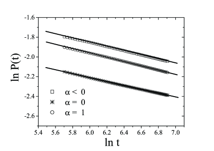
Figure 1: The numerical estimate of the probability $P(t)$ in (1) as described in the text.

For $r=10$ and $t=1000$ we obtain $\theta_{l}=0.2096(13)$. The same power law behavior was observed for $\alpha=0$ and $\alpha=1$, however with slightly different exponents, as can be seen in table 1.

	$\alpha<0$	$\alpha=0$	$\alpha=1$
$\theta_{l}$	0.2096(13)	0.1964(34)	0.1993(21)

Table 1: Local persistence exponent values of Blume Capel Model

For positive values of $\alpha$ ($\neq 1$) the system shows blocking, as can seen in figure 2. However a distinction must be made: in $\alpha\in$ $]0,1[$ the persistence has a fast decay and reaches a constant value $P(t\rightarrow\infty)\simeq 0.322$, while for $\alpha\in$ $]1,2]$ the value is $P(t\rightarrow\infty)\simeq 0.246$. For $\alpha=2$, $P(t\rightarrow\infty)\simeq 0.287$) and when $\alpha>2$ there is full blocking with $P(t\rightarrow\infty)$ frozen to the value $\simeq 0.333$ (initial mean fraction of spins is null). In $d=2$ and $T=0$ this is due to the fact that for $\alpha>2$ the predominant phase is a configuration with all spins zero.

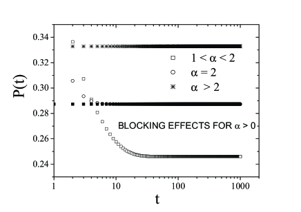
Figure 2: Blocking effects for positive values of $\alpha$ ($\neq 1$).

Our values for $\alpha<0$ are in agreement with more recent results for the Ising Model, namely

$$\theta_{l}=0.209(2)$$ (5)

jainflynm . The point $\alpha=0$ separates two distinct regions: a power law behavior for negative values of $\alpha$ and a blocking phase for positive values of this ratio. At $\alpha=0$ we have a power law behavior but with a different exponent.

Another interesting behavior is observed for $\alpha=1$, where a robust power law separates two different blocking ”phases”. The point $\alpha=2$ also divides two regions of distinct blocking behavior: the $1<\alpha<2$ region and the full–blocking region $\alpha>2$.

To conclude, our results show that nontrivial behavior in stochastic persistence can appear as one extends the Ising Model to allow for higher ”spins” and anisotropy effects as measured by our parameter $\alpha$. In particular for $\alpha<0$ one has a pure 2–state Ising behavior; the same is not observed for different values of $\alpha$, as discussed in the text. It would be interesting to test these ideas for different stochastic systems in the hope that there also nontrivial behavior might be found.

References

References

- (1) W. Feller, ” An Introduction to Probability Theory and Its Applications”, 1, John Whiley & Sons (1968)
- (2) B. Derrida, A. J. Bray, C. Godrèche, J. Phys. A 27, L357 (1994)
- (3) D. Stauffer, J. Phys. A 27, 5029 (1994)
- (4) S. N. Majumdar, A. J. Bray, S. J. Cornell, C. Sire 77 , 3704 (1996)
- (5) B. Derrida, Phys. Rev. E 55, 3705 (1997)
- (6) S. Jain, Phys. Rev. E 59 42493 (1999)
- (7) S. Jain, H. Flynn, J. Phys. A 33 8383 (2000)
- (8) R. da Silva, N. A. Alves, J. R. Drugowich de Felício, Phys. Rev. E 67, 057102 (2003)