Electromagnetic analog of Rashba spin-orbit interaction in wave guides filled with ferrite

Abstract

We consider infinitely long electromagnetic wave guide filled with a ferrite. The wave guide has arbitrary but constant cross-section $D$. We show that Maxwell equations are equivalent to the Schrödinger equation for single electron in the two-dimensional quantum dot of the form $D$ with account of the Rashba spin-orbit interaction. The spin-orbit constant is determining by components of magnetic permeability of the ferrite. The upper component of electron spinor function corresponds to the z-th component electric field, while the down component $\chi$ related to the z-th component of magnetic field by relation (30).

I Introduction

There is a complete equivalence of the two-dimensional Schrödinger equation for a particle in a hard wall box to microwave billiards stockmann . A wave function is exactly corresponds to the the electric field component of the TM mode of electromagnetic field: $\psi(x,y)\leftrightarrow E_{z}(x,y)$ with the same Dirichlet boundary conditions. This equivalence is turned out very fruitful and test a mass of predictions found in the quantum mechanics of billiards stockmann . In open systems the probability current density corresponds to the Poynting vector. The last equivalence allowed to test in particular universal current statistics in chaotic billiards barth ; saichev . Moreover if the resonator is non homogeneously filled with ferrite, a similarity to quantum billiards with broken time-reversal symmetry appears stockmann .

In present work we develop this idea of resonators filled with ferrite to show an equivalence of the Maxwell equations to electron in quantum dot (QD) with the Rashba spin-orbit interaction (SOI) rashba . This interaction is relevant in a two-dimensional electron gas, such as is formed in GaAs heterostructures. While spin-orbit scattering in metals is largely due to scattering from the metal ions or from impurities, in a GaAs heterostructure, spin-orbit effects mainly arise from the asymmetry of the potential creating the quantum well. The hamiltonian of single electron in the quantum dot with account of the Rashba SOI has the following form aronov ; morpugo

$$H=\frac{1}{2m^{*}}({\bf p}-\frac{e}{c}{\bf A})^{2}+\hbar K[{\bf\sigma\times(p}-\frac{e}{c}{\bf A})]_{z}$$ (1)

where $m^{*}=0.023m$ is the effective mass, $\hbar^{2}K=6\times 10^{-10}eV\cdot cm$ is the SOI coefficient in a InAs structures aronov . The dominant mechanism for the SOI in two-dimensional electron gas (2DEG) is attributed by the Rashba term rashba ; nitta . Using the characteristic scale of QD $R$ we rewrite (1) in dimensionless form for ${\bf B}=0$

$$\widetilde{H}=\left(\matrix{-\nabla^{2}&\beta(\frac{\partial}{\partial{x}}+i\frac{\partial}{\partial{y}})\cr\beta(-\frac{\partial}{\partial{x}}+i\frac{\partial}{\partial{y}})&-\nabla^{2}\cr}\right),$$ (2)

where $\beta=2m^{*}KR$. We consider that the electric field is directed normal to the plane of QD. If to introduce complex variables $\xi=x+iy$ and the Cauchy derivative $\frac{\partial}{\partial\xi}=\frac{1}{2}\left(\frac{\partial}{\partial x}-i\frac{\partial}{\partial y}\right)$ the the Schrödinger equation with the Hamiltonian (2) takes the following form

$$\left(\frac{\partial^{2}}{\partial\xi\partial\xi^{*}}+\frac{1}{4}\epsilon\right)\phi+\frac{\beta}{2}\frac{\partial{\chi}}{\partial\xi}=0,$$

$$\left(\frac{\partial^{2}}{\partial\xi\partial\xi^{*}}+\frac{1}{4}\epsilon\right)\chi-\frac{\beta}{2}\frac{\partial{\phi}}{\partial{\xi^{*}}}=0,$$ (3)

where $\phi,\chi$ are the components of the spin state and $\epsilon$ is the eigen energy.

II Basic electromagnetic equations

Let us consider electromagnetic waves in a wave guide filled with a ferrite with a magnetization $M_{0}$ directed along the z axis and with the following magnetic permutability

$$\hat{\mu}=1+4\pi\hat{\chi},$$

$$\hat{\chi}=\left(\matrix{\chi_{xx}&\chi_{xy}&0\cr-\chi_{xy}&\chi_{xx}&0\cr 0&0&\chi_{zz}\cr}\right).$$ (4)

By relation ${\bf B}=\hat{\mu}{\bf H}$ the Maxwell equations take the following form

$$\left(\frac{\partial{E_{z}}}{\partial y}-\frac{\partial{E_{y}}}{\partial z}\right)=-ik(\mu_{xx}H_{x}+\mu_{xy}H_{y}),$$

$$\left(\frac{\partial{E_{x}}}{\partial z}-\frac{\partial{E_{z}}}{\partial x}\right)=-ik(\mu_{yx}H_{x}+\mu_{yy}H_{y}),$$ (5)

$$\left(\frac{\partial{E_{y}}}{\partial x}-\frac{\partial{E_{x}}}{\partial y}\right)=-ik\mu_{zz}H_{z};$$

$$\left(\frac{\partial{H_{z}}}{\partial y}-\frac{\partial{H_{y}}}{\partial z}\right)=ikE_{x},$$

$$\left(\frac{\partial{H_{x}}}{\partial z}-\frac{\partial{H_{z}}}{\partial x}\right)=ikE_{y},$$ (6)

$$\left(\frac{\partial{H_{y}}}{\partial x}-\frac{\partial{H_{x}}}{\partial y}\right)=ikE_{z},$$

where frequency of electromagnetic waves $\omega=ck$. The first couple of the Maxwell equations $\nabla{\bf E}=0,\nabla{\bf B}=0$ follows from the second couple of equations (II) and (II).

Let us consider the wave guide infinitely long in $z$ direction. We take that a cross-section of the wave guide is constant in $x,y$ plane as shown in Fig. 1.

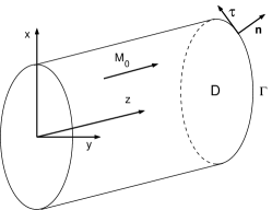
Figure 1: Schematical view of electromagnetic wave guide with constant cross-section

Such a geometry of the waveguide allows to separate variables $z$ and $x,y$ and write

$${\bf E}(x,y,z)=e^{ik_{z}z}{\bf E}(x,y),\quad{\bf H}(x,y,z)=e^{ik_{z}z}{\bf H}(x,y).$$ (7)

Then Eqs II reduce to

$$\frac{\partial}{\partial y}\left(\frac{\partial{H_{z}}}{\partial y}-\frac{\partial{H_{y}}}{\partial z}\right)-\frac{\partial}{\partial x}\left(\frac{\partial{H_{x}}}{\partial z}-\frac{\partial{H_{z}}}{\partial x}\right)=ik\frac{\partial{E_{x}}}{\partial y}-ik\frac{\partial{E_{y}}}{\partial x}.$$ (8)

Combining this equation with the third equation of (II) we obtain from (8)

$$\nabla_{\bot}^{2}H_{z}-\frac{\partial}{\partial z}\left(\frac{\partial{H_{x}}}{\partial x}+\frac{\partial{H_{y}}}{\partial y}\right)+k^{2}\mu_{zz}H_{z}=0,$$ (9)

where $\nabla_{\bot}=\frac{\partial^{2}}{\partial x^{2}}+\frac{\partial^{2}}{\partial y^{2}}$ is the two-dimensional Laplace operator.

The next task is to exclude $H_{y}$ and $H_{x}$ from (9). Eq. $\nabla{\bf B}=0$ gives

$$\mu_{xx}\left(\frac{\partial{H_{x}}}{\partial x}+\frac{\partial{H_{y}}}{\partial y}\right)+\mu_{xy}\left(\frac{\partial{H_{y}}}{\partial x}-\frac{\partial{H_{x}}}{\partial y}\right)+\mu_{zz}\frac{\partial{H_{z}}}{\partial z}=0.$$ (10)

Substituting the third equation (II) into (10) we obtain

$$-\left(\frac{\partial{H_{x}}}{\partial x}+\frac{\partial{H_{y}}}{\partial y}\right)=\frac{\mu_{zz}}{\mu_{xx}}\frac{\partial{H_{z}}}{\partial z}+ik\frac{\mu_{xy}}{\mu_{xx}}E_{z}.$$

Substituting this equation into (9) we obtain finally the first equation for $E_{z}$ and $H_{z}$:

$$\nabla_{\bot}^{2}H_{z}(x,y)+\left\{-k_{z}^{2}\frac{\mu_{zz}}{\mu_{xx}}+k^{2}\mu_{zz}\right\}H_{z}(x,y)-kk_{z}\frac{\mu_{xy}}{\mu_{xx}}E_{z}(x,y)=0.$$ (11)

Let us derive the next equation for $E_{z}$ and $H_{z}$. The first couple of equations (II) gives us:

$$\frac{\partial}{\partial y}\left(\frac{\partial{E_{z}}}{\partial y}-\frac{\partial{E_{y}}}{\partial z}\right)-\frac{\partial}{\partial x}\left(\frac{\partial{E_{x}}}{\partial z}-\frac{\partial{E_{z}}}{\partial x}\right)=-ik\frac{\partial}{\partial y}(\mu_{xx}H_{x}+\mu_{xy}H_{y})+ik\frac{\partial}{\partial x}(\mu_{yx}H_{x}+\mu_{yy}H_{y}).$$ (12)

Because of Eqs (II), (II) and (7) this equation can be written as follows

$$(\nabla_{\bot}^{2}+\mu_{xx}k^{2}-k_{z}^{2})E_{z}=ik\mu_{yx}\left(\frac{\partial{H_{x}}}{\partial x}+\frac{\partial{H_{y}}}{\partial y}\right).$$ (13)

On the other hand, Eq. $\nabla{\bf B}=0$ gives

$$\mu_{xx}\left(\frac{\partial{H_{x}}}{\partial x}+\frac{\partial{H_{y}}}{\partial y}\right)+ik\mu_{xy}E_{z}+\mu_{zz}\frac{\partial{H_{z}}}{\partial z}=0.$$

As a result we obtain finally from (II) and (13) the second equation for $E_{z}$ and $H_{z}$:

$$\left\{\nabla_{\bot}^{2}+(\mu_{xx}k^{2}-k_{z}^{2})+k^{2}\frac{\mu_{xy}}{\mu_{xx}}\right\}E_{z}+kk_{z}\frac{\mu_{xy}}{\mu_{xx}}H_{z}=0.$$ (14)

III Boundary conditions

Let us consider the boundary conditions for these relevant electromagnetic fields $E_{z}$ and $H_{z}$. Assume that surface of the wave guide shown in Fig. 1 is perfect metal. The boundary conditions are the following

$$E_{z}(x,y)|_{{}_{\Gamma}}=0,\quad E_{\tau}(x,y)|_{{}_{\Gamma}}=0$$ (15)

where $\tau$ is the unit vector directed along the boundary $\Gamma$ in the wave guide cross-section. Our task is to express $E_{\tau}$ through the relevant fields $E_{z}$ and $H_{z}$. Write the Maxwell equations (II), (II) and (7) as follows

$$\frac{\partial{E_{z}}}{\partial y}-ik_{z}E_{y}=-ik(\mu_{xx}H_{x}+\mu_{xy}H_{y}),$$

$$ik_{z}E_{x}-\frac{\partial{E_{z}}}{\partial x}=-ik(\mu_{yx}H_{x}+\mu_{yy}H_{y})$$ (16)

and

$$ik_{z}H_{y}=\frac{\partial{H_{z}}}{\partial y}-ikE_{x},$$

$$ik_{z}H_{x}=\frac{\partial{H_{z}}}{\partial x}+ikE_{y}.$$ (17)

From these equations we can express fields $E_{x}$ and $E_{y}$ via the fields $E_{z}$ and $H_{z}$. A tedious but straightforward algebra gives the following equations:

$$E_{x}=\frac{1}{D}\Bigg{\{}\left(\frac{\partial{H_{z}}}{\partial x}\right)[-ik^{3}\mu_{xy}\mu_{xx}-ik\mu_{xy}(k_{z}^{2}-k^{2}\mu_{xx})]$$

$$+\left(\frac{\partial{H_{z}}}{\partial y}\right)[-ik^{3}\mu_{xy}^{2}+ik\mu_{xx}(k_{z}^{2}-k^{2}\mu_{xx})]-ik_{z}k^{2}\mu_{xy}\left(\frac{\partial{E_{z}}}{\partial y}\right)-ik_{z}(k_{z}^{2}-k^{2}\mu_{xx})\left(\frac{\partial{E_{z}}}{\partial x}\right)\Bigg{\}},$$

$$E_{y}=\frac{1}{D}\Bigg{\{}\left(\frac{\partial{H_{z}}}{\partial x}\right)[+ik^{3}\mu_{xy}^{2}-ik\mu_{xx}(k_{z}^{2}-k^{2}\mu_{xx})]$$

$$+\left(\frac{\partial{H_{z}}}{\partial y}\right)[-ik^{3}\mu_{xx}\mu_{xy}-ik\mu_{xy}(k_{z}^{2}-k^{2}\mu_{xx})]+ik_{z}k^{2}\mu_{xy}\left(\frac{\partial{E_{z}}}{\partial x}\right)-ik_{z}(k_{z}^{2}-k^{2}\mu_{xx})\left(\frac{\partial{E_{z}}}{\partial y}\right)\Bigg{\}},$$ (18)

where $D=k^{4}\mu_{xy}^{2}+(k_{z}^{2}-k^{2}\mu_{xx})^{2}$.

Since $\overrightarrow{\tau}=(-n_{y}n_{x})$, the second boundary condition (15) takes the following form $-n_{y}E_{x}+n_{x}E_{y}|_{{}_{\Gamma}}=0$. Taking into account the first boundary condition (15) we obtain finally from (18)

$$\mu_{xy}\left\{kk_{z}\left(\frac{\partial{E_{z}}}{\partial n}\right)-k_{z}^{2}(\overrightarrow{\tau}\nabla_{\bot}H_{z})\right\}+\left(\frac{\partial{H_{z}}}{\partial n}\right)[k^{2}(\mu_{xy}^{2}+\mu_{xx}^{2})-k_{z}^{2}\mu_{xx}]|_{{}_{\Gamma}}=0$$

$$E_{z}|_{{}_{\Gamma}}=0.$$ (19)

IV SOI equivalent microwave equations

In order to write Eqs (11) and (14) in form equivalent to the Schrödinger equation (I) with the Rashba SOI let us introduce the following notations

$$h_{z}=iH_{z},$$

$$\epsilon_{1}=k^{2}-\frac{k_{z}^{2}}{\mu_{xx}},$$

$$\epsilon_{2}=k^{2}\mu_{xx}-k_{z}^{2}+\frac{k^{2}\mu_{xy}^{2}}{\mu_{xx}},$$

$$\nu=kk_{z}\kappa,\quad i\kappa=\frac{\mu_{xy}}{\mu_{xx}},$$ (20)

where lax

$$\mu_{xx}(\omega)=1+\frac{4\pi M_{0}\omega_{0}\Omega}{\Omega^{2}-\omega^{2}},\quad\mu_{xy}(\omega)=i\frac{4\pi M_{0}\omega_{0}\omega}{\Omega^{2}-\omega^{2}},$$ (21)

$$\omega_{0}=\gamma(H_{0}-4\pi M_{0}),$$

$$\Omega^{2}=\omega_{0}(\omega_{0}+\gamma H_{a}),$$

$$H_{a}=8\pi K_{a}/M.$$

Here $H_{0}$ is external constant magnetic field applied along the z-axis, i.e. along the direction of magnetization $M_{0}$ and $H_{a}$ is effective anisotropy field directed along the x-axis.

Let us introduce an auxiliary function $u_{2}(x,y)$:

$$h_{z}=\lambda\frac{\partial{u_{2}}}{\partial{\xi}},$$ (22)

where $\xi=x+iy$, and $\lambda$ is some coefficient which will be determined below . Then Eqs (11) and (14) take the following form

$$\left(4\frac{\partial^{2}}{\partial\xi\partial\xi^{*}}+\epsilon_{2}\right)E_{z}+\lambda\nu\frac{\partial{u_{2}}}{\partial{\xi}}=0,$$

$$\left(4\frac{\partial^{2}}{\partial\xi\partial\xi^{*}}+\epsilon_{1}\right)\lambda\frac{\partial{u_{2}}}{\partial{\xi}}+\nu E_{z}=0.$$ (23)

The first equation (IV) can be written as

$$E_{z}=-\frac{1}{\epsilon_{2}}\left(4\frac{\partial^{2}}{\partial\xi\partial\xi^{*}}+\lambda\nu\frac{\partial{u_{2}}}{\partial{\xi}}\right).$$ (24)

Let us choose $\lambda^{2}=4/\epsilon_{2}$. Then the second equation (IV) takes the following form

$$\frac{\partial}{\partial{\xi}}\left\{\Bigg{[}4\frac{\partial^{2}}{\partial\xi\partial\xi^{*}}+\left(\epsilon_{1}-\frac{\nu^{2}}{\epsilon_{2}}\right)\Bigg{]}u_{2}-\frac{2\nu}{\sqrt{\epsilon_{2}}}\frac{\partial{E_{z}}}{\partial{\xi^{*}}}\right\}=0.$$ (25)

The solution of equation $\frac{\partial g}{\partial{\xi}}=0$ is any function $g=g(\xi^{*})$ to give us the following equation:

$$\Bigg{[}4\frac{\partial^{2}}{\partial\xi\partial\xi^{*}}+\left(\epsilon_{1}-\frac{\nu^{2}}{\epsilon_{2}}\right)\Bigg{]}u_{2}-\frac{2\nu}{\sqrt{\epsilon_{2}}}\frac{\partial{E_{z}}}{\partial{\xi^{*}}}=g(\xi^{*}).$$ (26)

One can see that the magnetic field (22) is invariant under gauge transformations $u_{2}\rightarrow\chi=u_{2}+f(\xi^{*})$. Let us make this gauge transformation and substitute into Eq. (26). Then we obtain the following equation for transformed $\chi$:

$$4\frac{\partial^{2}{\chi}}{\partial\xi\partial\xi^{*}}+\left(\epsilon_{1}-\frac{\nu^{2}}{\epsilon_{2}}\right)\chi-\frac{2\nu}{\sqrt{\epsilon_{2}}}\frac{\partial{E_{z}}}{\partial{\xi^{*}}}=0,$$ (27)

provided that we have chosen the gauge as follows:

$$\left(\epsilon_{1}-\frac{\nu^{2}}{\epsilon_{2}}\right)f(\xi^{*})=g(\xi^{*}).$$ (28)

Finally combining this equation with the first equation (IV) we obtain the following system of equations

$$\left(\frac{\partial^{2}}{\partial\xi\partial\xi^{*}}+\frac{1}{4}\epsilon_{2}\right)E_{z}+\frac{\nu}{2\sqrt{\epsilon_{2}}}\frac{\partial{\chi}}{\partial{\xi}}=0,$$

$$\left(\frac{\partial^{2}}{\partial\xi\partial\xi^{*}}+\frac{1}{4}\left(\epsilon_{1}-\frac{\nu^{2}}{\epsilon_{2}}\right)\right)\chi-\frac{\nu}{2\sqrt{\epsilon_{2}}}\frac{\partial{E_{z}}}{\partial{\xi^{*}}}=0.$$ (29)

If to compare these equations with the Schrödinger equation for electron in quantum dot with SOI (I) one can see that the electric field $E_{z}$ is equivalent to the upper spinor component $\phi$ while $\chi$ is down component which related to magnetic field by relation

$$H_{z}=-\frac{2i}{\sqrt{\epsilon_{2}}}\frac{\partial{\chi}}{\partial{\xi}}.$$ (30)

The parameter $\frac{\nu}{\sqrt{\epsilon_{2}}}$ is completely equivalent to the SOI constant $\beta$. If to substitute relations (IV) one can see that Eq. (IV) is the equation for eigen functions $E_{z}$ and $\chi$ and eigenvalues $k^{2}$. The eigenvalues of Eq. (IV) will coincide with the eigenenergies of Eq. (I) if to choose by variation of magnetic permutability $\mu_{xx},\mu_{xy}$ and $k_{z}$

$$\epsilon_{2}=\epsilon_{1}-\frac{\nu^{2}}{\epsilon_{2}},$$ (31)

we can obtain exact correspondence between Eq. (I) and (IV). Only difference in boundary conditions is remaining.

This work has been partially supported by Russian Foundation for Basic research Grant 03-02-17039.

References

• (1) H.-J. StΓΆkmann, Quantum Chaos: An Introduction (Cambridge University Press, Cambridge, UK, 1999).
• (2) M. Barth and H.-J. StΓΆkmann, Phys. Rev. E 65, 066208 (2002).
• (3) A.I.Saichev, H.Ishio, A.F.Sadreev, and K.-F.Berggren, J. Phys. A: Math. and General,35, L87 (2002).
• (4) Yu. A. Bychkov and E. I. Rashba, JETP Lett. 39, 78 (1984). [5] A.
• (5) G. Aronov and Y. B. Lyanda-Geller, Phys. Rev. Lett. 70, 343 (1993).
• (6) A. F. Morpurgo, J. P. Heida, T. M. Kwapwijk, B. J. van Wees, and G. Borghs, Phys. Rev. Lett. 80, 1050 (1998).
• (7) J.Nitta, T.Akazaki, and H.Takayanagi, Phys. Rev. Lett., 78, 1335 (1997).
• (8) C. Kittel, Phys. Rev. 73, 155 (1948).
• (9) B. Lax, K.J. Button, Microwave Ferrites and Ferrimagnetics, N.Y., 1962.
• (10) B. Eckhard, J. Ford, and F. Vivaldi, Physica 13D, 339 (1984).