Nonequilibrium Superconductivity near Spin Active Interfaces

Abstract

The Riccati formulation of the quasiclassical theory of nonequilibrium superconductors is developed for spin-dependent scattering near magnetic interfaces. We derive boundary conditions for the Riccati distribution functions at a spin-active interface. The boundary conditions are formulated in terms of an interface S-matrix describing the reflection and transmission of the normal-state conduction electrons by the interface. The S-matrix describes the effects of spin-filtering and spin-mixing (spin-rotation) by a ferromagnetic interface. The boundary conditions for the Riccati equations are applicable to a wide range of nonequilibrium transport properties of hybrid systems of superconducting and magnetic materials. As an application we calculate the spin and charge conductance of a normal metal-ferromagnet-superconductor (NFS) point contact; the spin-mixing angle that parameterizes the S-matrix is determined from experimental measurements of the peak in the sub-gap differential conductance of the NFS point contact. We also use the new boundary conditions to derive the effects of spin-mixing on the phase-modulated thermal conductance of a superconducting-ferromagnetic-superconducting (SFS) point contact. For high-transparency (metallic ferromagnet) “$\pi$” junctions, the phase modulation of the thermal conductance is dramatically different from that of non-magnetic, “0” junctions. For low-transparency (insulating ferromagnet) SFS tunnel junctions with weak spin mixing resonant transmission of quasiparticles with energies just above the gap edge leads to an increase of the thermal conductance, compared to the normal-state conductance at $T_{c}$, over a broad temperature range when the superconducting phase bias is $\phi\gtrsim\pi/2$.

I Introduction

Spin dependent transport in hybrid systems composed of superconductors and spin-active materials such as ferromagnets has attracted a lot of attention because of the possibility of generating coherent spin transport for spintronic devices.Wolf et al. (2001) The spin polarization of a ferromagnetic material, one of the key parameters in the development of spintronic devices, is usually measured either by spin-dependent tunnelling techniques,Tedrow and Meservey (1994) or by point-contact Andreev reflection spectroscopy.Soulen et al. (1998) Both methods infer information about the spin polarization from the conductance data of superconductor-ferromagnet (SF) junctions. When sandwiched between two $s$-wave superconducting leads (an SFS junction), a ferromagnetic layer can produce a “$\pi$ junction”, i.e. a ground state of an SFS junction in which there is a $\pi$ phase difference between the two superconductors.Buzdin et al. (1982); Buzdin and Kupriyanov (1991) The $\pi$ state has been observed in SFS junctions with metallic ferromagnetic layers.Ryazanov et al. (2001); Kontos et al. (2002); Guichard et al. (2003) It is predicted theoretically that an insulating or semiconducting ferromagnetic layer can also produce a $\pi$ junction.M. Fogelström (2000); Barash and Bobkova (2002) More complicated $\pi$ junctions in which the Josephson coupling is provided by an inhomogeneous magnetization, e.g. a ferromagnet-insulator-ferromagnet (FIF) tri-layer, have also been investigated theoretically.Koshina and Krivoruchko (2001); Bergeret et al. (2001); Golubov et al. (2002); Barash et al. (2002)

The study of SFS junctions is fuelled in part by the proposal that $\pi$ junctions can be used to construct a non-dissipative superconducting phase qubit.Blatter et al. (2001) Most theoretical investigations of SFS junctions are restricted to equilibrium properties, however the performance of a $\pi$ junction as a qubit depends sensitively on the suppression of dissipative dynamics under nonequilibrium conditions. Recently, the nonequilibrium transport properties of Josephson junctions with spin active interfaces have begun to be explored theoretically.Andersson et al. (2002)

A powerful formulism for calculating the nonequilibrium properties of superconducting heterostructures is provided by the quasiclassical theory of superconductivity.Eliashberg (1972); Larkin and Ovchinnikov (1976); Serene and Rainer (1983); Rammer and Smith (1986) Traditionally one obtains the quasiclassical Green’s functions by solving the transport equations subject to boundary conditions at surfaces or interfaces.

A multi-step approach to the boundary value problem at a surface or interface based on an interface transition matrix has been used by several authors.Serene and Rainer (1983); Kieselmann (1985); Cuevas and Fogelström (2001); Eschrig et al. (2003); Kopu et al. (2004) This method requires one to calculate an auxiliary Green’s function for an impenetrable surface. The auxiliary Green’s function is then used as an input to a T-matrix equation from which one constructs the quasiclassical Green’s functions at the interface. This method can be applied to a broad class of interface models, and is suitable for numerical computations,Cuevas and Fogelström (2001); Eschrig et al. (2003); Kopu et al. (2004) but it requires the computation of intermediate, unphysical auxiliary Green’s functions.

Boundary conditions which are expressed only in terms of the physical quasiclassical propagators and interface reflection and transmission amplitudes have been derived from microscopic scattering theory by ZaitsevZaĭtsev (1984) and KieselmannKieselmann (1985) for nonmagnetic interfaces, and for spin active interfaces by Millis, Rainer and one of the authors.Millis et al. (1988) These boundary conditions are formulated as a set of third order equations in terms of the matrix Green’s functions at the boundary, connected via an interface scattering matrix (S-matrix) for normal metal electrodes. Although auxiliary propagators are not present, the nonlinear boundary conditions are non-intuitive, difficult to solve and contain unphysical solutions which must be discarded.

Recently, a more intuitive and computationally efficient form of the quasiclassical boundary conditions was obtained for non-magnetic interfaces by Eschrig.Eschrig (2000) This formulation starts from the boundary condition of Zaitsev and Kieselmann, and is obtained by parameterizing the quasiclassical Green’s functions in terms of Riccati amplitudes.Schopohl and Maki (1995); Schopohl (1996); Eschrig et al. (1999); Shelankov and Ozana (2000); Eschrig (2000) By formulating the quasiclassical theory in terms of the Riccati amplitudes, not only are the transport equations easier to solve numerically, but the boundary conditions become linear and free of spurious solutions.Eschrig (2000) Eschrig’s formulation of the boundary condition amounts to finding physical solution to the Zaitsev-Kieselmann nonlinear boundary condition. For spin-active interfaces Fogelström obtained boundary conditions for the retarded and advanced coherence functions.M. Fogelström (2000) However, a complete set of boundary conditions for non-equilibrium transport with spin-active interfaces was lacking.

In this paper we derive the boundary condition for the quasiclassical Riccati amplitudes, both the coherence functions and distribution functions, for spin active interfaces and apply the new boundary conditions to study the nonequilibrium transport properties of clean superconductor-ferromagnet hybrid systems. The paper is organized as follows. The complete set of boundary conditions for the Riccati amplitudes at spin active interfaces is presented in section II, with technical steps of the derivation described in an appendix. In section III, the S-matrix for scattering by two models for spin-active interfaces, a ferromagnetic-insulating layer and a ferromagnetic-metallic layer, are derived and discussed in terms of the effects of spin filtering and spin mixing. Applications of the theory to the conductance of the normal metal-ferromagnet-superconductor junction is analyzed in section IV. In section V the influence of spin mixing on the phase sensitive heat transport in SFS point contact is discussed in detail.

II The boundary conditions for Riccati amplitudes

In the Riccati formulation of the quasiclassical theory of nonequilibrium superconductivity, the quasiparticle excitation spectrum is determined from coherence functions, $\gamma^{R,A}$ and $\tilde{\gamma}^{R/A}$, which measure the relative amplitudes for normal-state quasi-particle and quasi-hole excitations; the occupation probability of theses states is described by distribution functions, $x^{K}$ and $\tilde{x}^{K}$.Schopohl and Maki (1995); Schopohl (1996); Eschrig et al. (1999); Shelankov and Ozana (2000); Eschrig (2000) For brevity we refer to both types of functions as Riccati amplitudes, or Riccati functions, since all obey Riccati-type transport equations, defined on classical trajectories in phase space ($\mathbf{p},\mathbf{R}$). Thus, in general the Riccati amplitudes are functions of space, $\mathbf{R}$, time, $t$, the direction of the Fermi momentum, $\mathbf{p}_{f}$ (or Fermi velocity $\mathbf{v}_{f}$) and the excitation energy, $\epsilon$.

The Riccati amplitudes depend on spin, and in general are described by $2\times 2$ density matrices in spin space whose eigenvalues determine the local coherence and distribution functions for two possible spin states. The coherence amplitudes obey Riccati-type equations; for example,

$$i\mathbf{v}_{f}\cdot\mathbf{\nabla}\gamma^{R}=-2\epsilon\gamma^{R}+\gamma^{R}\tilde{\Delta}\gamma^{R}+\Sigma^{R}\gamma^{R}-\gamma^{R}\tilde{\Sigma}^{R}-\Delta^{R}\,.$$ (1)

The distribution function, $x^{K}$, obeys a Riccati-type transport equation,

$$i(\partial_{t}+\mathbf{v}_{f}\cdot\mathbf{\nabla})x^{K} = (\gamma^{R}\tilde{\Delta}^{R}+\Sigma^{R})x^{K}$$ (2)

$$+ x^{K}(\Delta^{A}\tilde{\gamma}^{A}-\Sigma^{A})$$

$$- \gamma^{R}\tilde{\Sigma}^{K}\tilde{\gamma}^{A}-\Sigma^{K}$$

$$+ \Delta^{K}\tilde{\gamma}^{A}+\gamma^{R}\tilde{\Delta}^{K}\,,$$

where $\Sigma^{\mu}$ and $\Delta^{\mu}$, $\mu=R,A,K$, are the diagonal and off-diagonal self-energies, respectively. We follow the notation in Ref. Eschrig, 2000 throughout the paper. Particle$\leftrightarrow$hole conjugation, denoted by $\tilde{}$, is defined by the operation $\tilde{q}(\hat{\mathbf{p}}_{f},\epsilon)=q^{*}(-\hat{\mathbf{p}}_{f},-\epsilon)$. The product of two functions of energy and time is defined by the non-commutative convolution,

$$AB\equiv A\circ B(\epsilon,t)=e^{i(\partial^{A}_{\epsilon}\partial^{B}_{t}-\partial^{A}_{t}\partial^{B}_{\epsilon})/2}A(\epsilon,t)B(\epsilon,t)\,.$$ (3)

Neither the operator, $\circ$, nor the arguments, $(\epsilon,t)$, are shown explicitly unless required.

Once the Riccati equations are solved subject to appropriate boundary conditions, the quasiclassical Green’s functions can be constructed from the Riccati amplitudes. Physical observables such as the charge or heat current can then be calculated. This procedure is discussed extensively by several authors, c.f. Refs. Eschrig et al., 1999; Eschrig, 2000.

At an interface or surface the local electronic potential changes on an atomic length and energy scales. Such strong, short-range potentials are treated within the quasiclassical theory as boundary conditions for the quasiclassical Green’s functions, or equivalently the Riccati amplitudes. Such an interface can be described by a scattering matrix, $\mathcal{S}$, for normal-state electrons and holes with excitation energies near the Fermi surface.Millis et al. (1988) Here we confine our discussion to specular interfaces, in which case the momentum of an excitation parallel to the interface, $\mathbf{p}_{||}$, is conserved. The interface $\mathcal{S}$ matrix is then described by a unitary matrix in the combined spin, particle-hole and direction spaces. Thus,

$$\mathcal{S}(\hat{\mathbf{p}}_{f})=\left(\begin{array}[]{cc}\hat{S}_{11}&\hat{S}_{12}\\ \hat{S}_{21}&\hat{S}_{22}\end{array}\right)\,,$$ (4)

where the index 1 (2) refers to the left (right) side of the interface. Each element of this matrix, $\hat{S}_{ij}$, is a diagonal Nambu matrix in particle-hole space,

$$\hat{S}_{ij}=\left(\begin{array}[]{cc}S_{ij}&0\\ 0&\underline{S}_{ij}\end{array}\right),\;i,j=1,2;$$ (5)

in which $S_{ij}$ and $\underline{S}_{ij}$ are matrices in spin space, which are related by particle-hole conjugation, $\underline{S}_{ij}(\mathbf{p}_{\parallel})=[S_{ji}(-\mathbf{p}_{\parallel})]^{\text{tr}}$, where $[..]^{\text{tr}}$ is the matrix transpose in spin space.Millis et al. (1988)

Figure 1: The Riccati amplitudes corresponding to the scattering trajectories for a partially transmitting specular interface. The interface normal is $\hat{z}$. The trajectories for the scattering states are labelled $1i,1o,2i$ and $2o$.

The Riccati amplitudes for the set of scattering trajectories labelled $1i,1o,2i$ and $2o$, shown in Fig. 1, are classified into two groups. The quantities $\{\gamma^{R,A}_{j},\tilde{\gamma}^{R,A}_{j},x^{K}_{j},\tilde{x}^{K}_{j}\}$, denoted by lower case symbols, are obtained by integrating the Riccati equations along the four trajectories from the bulk toward the interface. The quantities $\{\Gamma^{R,A}_{j},\tilde{\Gamma}^{R,A}_{j},X^{K}_{j},\tilde{X}^{K}_{j}\}$, denoted by upper case symbols, are obtained by starting at the interface and integrating along the trajectory into the bulk. The boundary conditions listed below connect the unknown upper case amplitudes at the interface with the known lower case amplitudes via the interface scattering matrix. The derivation of these boundary conditions is outlined in the appendix. For example, the boundary conditions for trajectory $1o$ are,

$$\Gamma^{R}_{1} = r^{R}_{1l}\gamma^{R}_{1}\underline{S}^{\dagger}_{11}+t^{R}_{1l}\gamma^{R}_{2}\underline{S}^{\dagger}_{12}\,,$$ (6)

$$\tilde{\Gamma}^{A}_{1} = \underline{S}_{11}\tilde{\gamma}^{A}_{1}\tilde{r}^{A}_{1r}+\underline{S}_{12}\tilde{\gamma}^{A}_{2}\tilde{t}^{A}_{1r}\,,$$ (7)

$$X^{K}_{1} = r^{R}_{1l}x^{K}_{1}\tilde{r}^{A}_{1r}+t^{R}_{1l}x^{K}_{2}\tilde{t}^{A}_{1r}-a^{R}_{1l}\tilde{x}^{K}_{2}\tilde{a}^{A}_{1r}\,,$$ (8)

where we have introduced effective reflection ($r$), transmission ($t$) and branch-conversion transmission ($a$) amplitudes,

$$r^{R}_{1l} = +[(\beta^{R}_{21})^{-1}S^{\dagger}_{11}-(\beta^{R}_{22})^{-1}S^{\dagger}_{12}]^{-1}(\beta^{R}_{21})^{-1}\,,$$ (9)

$$t^{R}_{1l} = -[(\beta^{R}_{21})^{-1}S^{\dagger}_{11}-(\beta^{R}_{22})^{-1}S^{\dagger}_{12}]^{-1}(\beta^{R}_{22})^{-1}\,,$$ (10)

$$\tilde{r}^{A}_{1r} = +(\beta^{A}_{21})^{-1}[S_{11}(\beta^{A}_{21})^{-1}-S_{12}(\beta^{A}_{22})^{-1}]^{-1}\,,$$ (11)

$$\tilde{t}^{A}_{1r} = -(\beta^{A}_{22})^{-1}[S_{11}(\beta^{A}_{21})^{-1}-S_{12}(\beta^{A}_{22})^{-1}]^{-1}\,,$$ (12)

$$a^{R}_{1l} = (\Gamma^{R}_{1}\underline{S}_{11}-S_{11}\gamma^{R}_{1})(\tilde{\beta}^{R}_{12})^{-1}\,,$$ (13)

$$\tilde{a}^{A}_{1r} = (\tilde{\beta}^{A}_{12})^{-1}(\underline{S}^{\dagger}_{11}\tilde{\Gamma}^{A}_{1}-\tilde{\gamma}^{A}_{1}S^{\dagger}_{11})\,.$$ (14)

The auxiliary quantities, $\beta^{R/A}_{ij}$, are defined as

$$\beta^{R}_{ij} = S^{\dagger}_{ij}-\gamma^{R}_{j}\underline{S}^{\dagger}_{ij}\tilde{\gamma}^{R}_{i};\;\tilde{\beta}^{R}_{ij}=\underline{S}_{ji}-\tilde{\gamma}^{R}_{j}S_{ji}\gamma^{R}_{i}\,,$$ (15)

$$\beta^{A}_{ij} = S_{ij}-\gamma^{A}_{i}\underline{S}_{ij}\tilde{\gamma}^{A}_{j};\;\tilde{\beta}^{A}_{ij}=\underline{S}^{\dagger}_{ji}-\tilde{\gamma}^{A}_{i}S^{\dagger}_{ji}\gamma^{A}_{j}\,.$$ (16)

Similarly, for trajectory $1i$ we have

$$\tilde{\Gamma}^{R}_{1} = \tilde{r}^{R}_{1l}\tilde{\gamma}^{R}_{1}S_{11}+\tilde{t}^{R}_{1l}\tilde{\gamma}^{R}_{2}S_{21}\,,$$ (17)

$$\Gamma^{A}_{1} = S^{\dagger}_{11}\gamma^{A}_{1}r^{A}_{1r}+S^{\dagger}_{21}\gamma^{A}_{2}t^{A}_{1r}\,,$$ (18)

$$\tilde{X}^{K}_{1} = \tilde{r}^{R}_{1l}\tilde{x}^{K}_{1}r^{A}_{1r}+\tilde{t}^{R}_{1l}\tilde{x}^{K}_{2}t^{A}_{1r}-\tilde{a}^{R}_{1l}x^{K}_{2}a^{A}_{1r}\,,$$ (19)

where

$$\tilde{r}^{R}_{1l} = +[(\tilde{\beta}^{R}_{21})^{-1}\underline{S}_{11}-(\tilde{\beta}^{R}_{22})^{-1}\underline{S}_{21}]^{-1}(\tilde{\beta}^{R}_{21})^{-1}\,,$$ (20)

$$\tilde{t}^{R}_{1l} = -[(\tilde{\beta}^{R}_{22})^{-1}\underline{S}_{11}-(\tilde{\beta}^{R}_{22})^{-1}\underline{S}_{21}]^{-1}(\tilde{\beta}^{R}_{21})^{-1}\,,$$ (21)

$$r^{A}_{1r} = +(\tilde{\beta}^{A}_{21})^{-1}[\underline{S}^{\dagger}_{11}(\tilde{\beta}^{A}_{21})^{-1}-\underline{S}^{\dagger}_{21}(\tilde{\beta}^{A}_{22})^{-1}]^{-1}\,,$$ (22)

$$t^{A}_{1r} = -(\tilde{\beta}^{A}_{22})^{-1}[\underline{S}^{\dagger}_{11}(\tilde{\beta}^{A}_{21})^{-1}-\underline{S}^{\dagger}_{21}(\tilde{\beta}^{A}_{22})^{-1}]^{-1}\,,$$ (23)

$$\tilde{a}^{R}_{1l} = (\tilde{\Gamma}^{R}_{1}S^{\dagger}_{11}-\underline{S}^{\dagger}_{11}\tilde{\gamma}^{R}_{1})(\beta^{R}_{12})^{-1}\,,$$ (24)

$$a^{A}_{1r} = (\beta^{A}_{12})^{-1}(S_{11}\Gamma^{A}_{1}-\gamma^{A}_{1}\underline{S}_{11})\,.$$ (25)

The boundary conditions for trajectories $2i$ and $2o$ are given by interchanging indices $1\leftrightarrow 2$ in Eqs. (6)-(25). The derivation of Eqs. (6)-(25) is described in the appendix.

Note that there is more than one physically equivalent representation of the boundary condition for any of the coherence functions. For example, it is straightforward to show that an alternative form of the boundary condition in Eq. 6 for $\Gamma^{R}_{1}$ is given by

$$\Gamma^{R}_{1} = S_{11}\gamma^{R}_{1}r^{R}_{1r}+S_{12}\gamma^{R}_{2}t^{R}_{1r}$$ (26)

$$r^{R}_{1r} = +(\tilde{\beta}^{R}_{12})^{-1}[\underline{S}_{11}(\tilde{\beta}^{R}_{12})^{-1}-\underline{S}_{12}(\tilde{\beta}^{R}_{22})^{-1}]^{-1}$$ (27)

$$t^{R}_{1r} = -(\tilde{\beta}^{R}_{22})^{-1}[\underline{S}_{11}(\tilde{\beta}^{R}_{12})^{-1}-\underline{S}_{12}(\tilde{\beta}^{R}_{22})^{-1}]^{-1}\,.$$ (28)

Similar results for $\Gamma^{R,A}_{j}$ and $\tilde{\Gamma}^{R,A}_{j}$ were obtained by Fogelström.M. Fogelström (2000) Combined with these results for the coherence functions, the boundary conditions for distribution functions given in Eqs. (8) and (19) provide a complete set of quasiclassical boundary conditions applicable to a wide range of non-equilibrium conditions for superconductors in contact with spin-active interfaces. These boundary conditions (Eqs. (6)-(25)) reduce to the results of Ref. Eschrig, 2000 for non-spin-active scattering, i.e. when $S_{ij}$ and $\underline{S}_{ij}$ are spin-independent.

In deriving Eqs. (6)-(25) we assumed that the inverses of $\beta^{R/A}_{ij}$, and their $\tilde{\;}$ partners, are defined. Equations (6)-(25) cannot be applied when one or more of the $\mathcal{S}$ matrix elements is zero. However, in cases where this happens the boundary conditions are significantly simplified, and can be readily derived following the procedure outlined in the appendix. For example, in the case of an impenetrable wall, we have perfect reflection described by $S_{12}=S_{21}=0$. Then Eqs. (6)-(8) are replaced by the simpler set of boundary conditions,

$$\Gamma^{R}_{1} = S_{11}\gamma^{R}_{1}\underline{S}_{11}^{\dagger}$$ (29)

$$\tilde{\Gamma}^{A}_{1} = \underline{S}_{11}\tilde{\gamma}^{A}_{1}S_{11}^{\dagger}$$ (30)

$$X^{K}_{1} = S_{11}x^{K}_{1}S_{11}^{\dagger}\,.$$ (31)

Similarly for perfect transmission, $S_{jj}=0$, the boundary conditions simplify to

$$\Gamma^{R}_{1} = S_{12}\gamma^{R}_{2}\underline{S}_{12}^{\dagger}$$ (32)

$$\tilde{\Gamma}^{A}_{1} = \underline{S}_{12}\tilde{\gamma}^{A}_{2}S_{12}^{\dagger}$$ (33)

$$X^{K}_{1} = S_{12}x^{K}_{2}S_{12}^{\dagger}\,.$$ (34)

Further simplification occurs for stationary non-equilibrium transport. The time convolution products reduce to matrix products, and there are additional symmetry relations: $\beta^{A}_{ij}=(\beta^{R}_{ij})^{\dagger}$, $\tilde{\beta}^{A}_{ij}=(\tilde{\beta}^{R}_{ij})^{\dagger}$, $\tilde{r}^{A}_{1r}=(r^{R}_{1l})^{\dagger}$, $\tilde{t}^{A}_{1r}=(t^{R}_{1l})^{\dagger}$, and $\tilde{a}^{A}_{1r}=(a^{R}_{1l})^{\dagger}$.

III The $\mathcal{S}$ matrix

A microscopic calculation of the normal-state $\mathcal{S}$ matrix for a spin active interface would require a solution of the many-body problem in the presence of the interface potential. This is a formidable problem and outside the realm of a practical theory aimed at understanding the transport properties of heterogeneous superconducting junctions. The alternative approach is to identify the structure of the $\mathcal{S}$ matrix, including the constraints of symmetry, and then model the interface in terms of the key physical parameters defining these characteristics, e.g. the transmission and reflection probabilities for normal-state electrons and holes moving along specific trajectories and in particular spin states. For a relatively small set of physical parameters, the key characteristics of the interface can be obtained from measurements, e.g. from normal-state transport properties, and then used to make predictions for non-equilibrium properties in the superconducting state. This is the most tractable approach to interpreting and predicting the nonequilibrium properties of heterogeneous superconducting junctions.

In this section we discuss the parametrization of the $\mathcal{S}$ matrix in terms of a spin-mixing angle and spin-dependent normal-state transmission coefficients. Other authors have also discussed the form of this interface $\mathcal{S}$ matrix for particular magnetic interfaces, c.f. Refs. Tokuyasu et al., 1988; M. Fogelström, 2000; Barash and Bobkova, 2002; Barash et al., 2002 We discuss the form of the $\mathcal{S}$ matrix for both a ferromagnetic insulating interface and a clean ferromagnetic metallic interface. For both cases we assume the interface is atomically smooth so that the momentum parallel to the interface, $\mathbf{p}_{||}$, is a good quantum number.

First consider the $\mathcal{S}$ matrix of a ferromagnetic insulating or semiconducting (FI) interface.Tokuyasu et al. (1988); M. Fogelström (2000); Barash and Bobkova (2002) Choose the direction of the spontaneous magnetization $\hat{\mu}$ as the quantization axis for the conduction electron spin. Then spin up $(+)$ and down $(-)$ electrons see the FI interfaces as a potential barrier with thickness $l$ and height $E_{g}\mp h$, where $E_{g}$ is the average band gap and $h$ is the exchange energy. The effects of the FI layer on the transport of electrons are two fold: 1) spin filtering in which the reflection (transmission) probabilities for spin up and spin down electrons are different, because these electrons with different spin polarization see different potential barriers, and 2) spin mixing in which spin up and down electrons acquire different phase shifts upon reflection (transmission). This is the analog of circular birefringence in optics. Thus, in general the polarization of an incident electron undergoes a rotation analogous to optical Faraday rotation.

The degrees of spin filtering and spin mixing are determined by the modulus and the phase of the reflection (transmission) amplitudes, respectively. Consider the reflection amplitude for example. In the spinor basis $|\pm\rangle$ which diagonalizes $\hat{\mu}\cdot\vec{\sigma}$, the spin matrix $S_{11}$ is diagonal,

$$S_{11}=\left(\begin{array}[]{cc}r_{+}&0\\ 0&r_{-}\\ \end{array}\right)=\left(\begin{array}[]{cc}|r_{+}|e^{i\theta_{+}}&0\\ 0&|r_{-}|e^{i\theta_{-}}\\ \end{array}\right)\,.$$ (35)

For an arbitrary basis $S_{11}$ can be parameterized as

$$S_{11}=e^{i\varphi_{11}/2}[s_{11}+s^{\prime}_{11}(\hat{\mu}\cdot\vec{\sigma})]e^{i(\hat{\mu}\cdot\vec{\sigma})\vartheta_{11}/2}\,,$$ (36)

where the overall phase factor, $\varphi_{11}\equiv\theta^{r}_{+}+\theta^{r}_{-}$, and the spin mixing angle, $\vartheta_{11}\equiv\theta_{+}-\theta_{-}$, are defined as the sum and difference of the phases for the reflected spin up and spin down electrons. The two real amplitudes, $s_{11}=(|r_{+}|+|r_{-}|)/2$ and $s^{\prime}_{11}=(|r_{+}|-|r_{-}|)/2$, determine the spin filtering effect. A similar parametrization can be carried out for each element, $S_{ij}$, of the $\mathcal{S}$ matrix.

The unitary condition, $\mathcal{S}\mathcal{S}^{{\dagger}}=1$, combined with symmetries of the interface, provide constraints between the values of $\{\varphi_{ij},\vartheta_{ij},s_{ij},s^{\prime}_{ij}\}$. For a specular FI interface with inversion symmetry, the constraint of time reversal symmetry, which includes the reversal of the ferromagnetic moment, gives $\varphi_{21}=\varphi_{11}+\pi/2$, and $\vartheta_{21}=\vartheta_{11}$. In this case the spin mixing angle for reflection and transmission are the same. The resulting $\mathcal{S}$ matrix simplifies, and is conveniently expressed in the basis, $|\pm\rangle$,

$$S_{11}=S_{22}=\;e^{i\varphi/2}\left(\begin{array}[]{cc}\sqrt{R_{\uparrow}}e^{i\vartheta/2}&0\\ 0&\sqrt{R_{\downarrow}}e^{-i\vartheta/2}\\ \end{array}\right)$$ (39)

$$S_{21}=S_{12}=ie^{i\varphi/2}\left(\begin{array}[]{cc}\sqrt{D_{\uparrow}}e^{i\vartheta/2}&0\\ 0&\sqrt{D_{\downarrow}}e^{-i\vartheta/2}\\ \end{array}\right)\,,$$ (42)

where $R_{\alpha}+D_{\alpha}=1$, $\alpha=\uparrow$, $\downarrow$. The overall phase factor, $\varphi$, drops out of all observables in the quasiclassical approximation and can be omitted. Therefore the $\mathcal{S}$ matrix is described by three parameters: the transparencies for spin up and spin down electrons, $D_{\uparrow}$ and $D_{\downarrow}$, and the spin mixing angle, $\vartheta$.

If we also have reflection symmetry in a plane perpendicular to the interface, then $S_{ij}(-\mathbf{p_{\parallel}})=S_{ij}(\mathbf{p_{\parallel}})$. This implies that that the S matrix for hole scattering is simply $\underline{S}_{ij}=S_{ij}$. This model of a ferromagnetic interface defined by Eq. (42), as well as special cases without spin filtering, have been discussed previously by several authors.Tokuyasu et al. (1988); M. Fogelström (2000); Barash and Bobkova (2002) The reflection and transmission probabilities, $\{R_{\alpha},D_{\alpha},\vartheta\}$ are functions of the direction of the trajectory of an incident quasiparticle, $\hat{\mathbf{p}}_{f}$, and depend on material parameters such as the band gap, $E_{g}$, the Fermi velocities of the electrons in the two metallic leads, $\mathbf{v}_{fi}$, exchange field, $h$, barrier thickness, $l$, etc.

To illustrate the typical parameters for spin mixing and spin filtering by a FI interface consider a FI barrier with a band gap of $E_{g}=0.825$ eV and and exchange splitting of $h=0.18$ eV, between two metallic leads. For conduction electrons with effective mass $m^{*}$ equal to the band mass of carriers in the FI we can calculate the spin-mixing angle and the transmission probabilities for spin up and spin down conduction electrons at normal incidence. A barrier of width $l=0.5$ nm gives $D_{\uparrow}=0.013$, $D_{\downarrow}=0.007$, and $\vartheta=0.032\,\pi$. The ratio $D_{\downarrow}/D_{\uparrow}$ vanishes exponentially as the barrier thickness increases, and the spin mixing angle $\vartheta$ saturates at $0.0348\pi$, the spin mixing angle for a perfectly reflecting FI surface. For angles away from normal incidence the effective barrier thickness increases and the corresponding transmission probabilities decrease rapidly away from normal incidence as shown in Fig. 2. The spin mixing angle also decreases with the angle of incidence, and vanishes for grazing incidence.

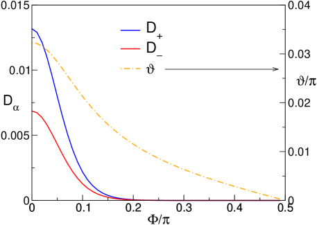
Figure 2: The spin up ($D_{+}$) and spin down ($D_{-}$) transmission probabilities, and the spin mixing angle as a function of the angle of incidence, $\Phi=\arccos(\hat{\mathbf{p}}_{f}\cdot\hat{z})$. The model parameters for the S-FI-S interface are described in the text.

The $\mathcal{S}$ matrix model in Eq. (42) is sufficiently general to account for the essential features of spin-active scattering by a clean, ferromagnetic metallic (FM) layer.Barash and Bobkova (2002) For example, assume the transmission and reflection of electrons by the interface is controlled by Fermi wave-vector mismatch at the S-FM interface. Upon entering the FM layer, the Fermi momenta for majority (spin up) and minority (spin down) electrons changes to $p_{f}^{\pm}=\sqrt{(E_{f}\pm h)2m^{*}}$, respectively. As a result the transmitted majority- and minority-spin electrons acquire a relative phase.

For sufficiently large angles of incidence the normal component of the momentum of the spin down electrons in the FM, $p_{z}^{-}=\sqrt{(E_{f}\cos^{2}\Phi-h)2m^{*}}$, vanishes and becomes imaginary for larger angles of incidence. Thus, these spin down electrons can only tunnel through the FM barrier. Since the charge and heat currents are dominated by trajectories close to normal incidence we consider the transmission probabilities and spin-mixing angle in the small angle limit near normal incidence, where both $p_{z}^{+}$ and $p_{z}^{-}$ are real. If we further assume the exchange field is relatively weak, $h\ll E_{f}$, then to the leading order in $h/E_{f}$,

$$\vartheta=\theta_{+}-\theta_{-}\simeq(p_{z}^{+}-p_{z}^{-})l$$ (43)

$$D_{\alpha}\simeq 1-(p_{z}^{\alpha}/p_{z}-p_{z}/p_{z}^{\alpha})^{2}\sin^{2}(p_{z}^{\alpha}l)/4\,.$$ (44)

Thus, for normal incidence the spin mixing angle is of order $\vartheta\sim p_{f}l\,(h/E_{f})$, which can easily approach $\vartheta\to\pi$. The electrons of both spin species are nearly perfectly transmitted, $D_{\alpha}\simeq 1-(h/2E_{f})^{2}$, and the spin filtering effect is negligibly small,

$${D_{\uparrow}-D_{\downarrow}\over D_{\uparrow}+D_{\downarrow}}\sim\mathcal{O}\left({h\over 2E_{f}}\right)^{3}\,.$$ (45)

Thus, the dominant effect of the FM interface is spin mixing, and an approximate form for the $\mathcal{S}$ matrix of an ideal FM interface is given by $S_{11}=S_{22}\simeq 0$ and

$$S_{12}=S_{21}\simeq e^{i\varphi}e^{i(\vec{\sigma}\cdot\hat{\mu})\vartheta/2}\,.$$ (46)

Starting from Eq. (46) a more detailed model for the $\mathcal{S}$ matrix of a FM interface can be constructed by adding a thin nonmagnetic insulating layer, with transparency $D$, inside the ideal FM, which may describe an interfacial dielectric barrier. The composite $\mathcal{S}$ matrix of this structure takes the form of Eq. (42) with $D_{\uparrow}=D_{\downarrow}=D$.

However, there presumably exist a wide variety of spin active interfaces, described by any physically allowed value of $\vartheta$ and $D_{\alpha}$. Thus, the calculations that follow are carried out for a broad range of values of $\vartheta$ and $D_{\alpha}$.

IV FM & FI point contacts

We now illustrate the application of the boundary conditions by calculating some representative transport properties for both NFS and SFS point contacts. These calculations highlight the role of the spin mixing angle in modifying the local spectrum near the point contact and in modifying the effective transmission coefficient for excitations that carry currents across the interface of the point contact.

Although the formalism is applicable to superconductors with any pairing symmetry, the calculations described here are for spin-singlet, $s$-wave superconductors. For a point contact the radius of the contact is much smaller than the coherence length. In this limit the pairbreaking effect of the FM on the magnitude of the order parameter can be neglected, and the voltage drop occurs at the contact because of the large Sharvin resistance.Zhao et al. (2003) Then at the point contact the Riccati amplitudes $\gamma^{R/A}_{j},\tilde{\gamma}^{R/A}_{j},x^{K}_{j},\tilde{x}^{K}_{j}$ take their local, bulk equilibrium values given by,Eschrig (2000)

$$\gamma^{R}_{j}(|\epsilon|<\Delta_{j})=-(i\sigma_{2})e^{-i\delta_{j}+i\phi_{j}},$$ (47)

$$\gamma^{R}_{j}(|\epsilon|>\Delta_{j})=-(i\sigma_{2})\mathrm{sgn}(\epsilon)e^{-\delta_{j}+i\phi_{j}},$$ (48)

$$x^{K}_{j}=(1-|\gamma_{j}^{R}|^{2})\tanh{\epsilon-eV_{j}\over 2T_{j}}$$ (49)

where we introduced the dimensionless parameters,

$$\delta_{j}=\arccos{\epsilon\over\Delta_{j}},\;|\epsilon|<\Delta_{j}$$ (50)

$$\cosh\delta_{j}={|\epsilon|\over\Delta_{j}},\;|\epsilon|>\Delta_{j}\,,$$ (51)

and $\Delta_{j}$ is the gap, $V_{j}$ is the potential, $T_{j}$ is the temperature, and $\phi_{j}$ is the phase of superconductor on side $j=1,2$. Application of the boundary conditions, Eqs. (6)-(25), is straight forward; we obtain $\Gamma^{R/A}_{j}$, $\tilde{\Gamma}^{R/A}_{j}$, $X^{K}_{j}$ and $\tilde{X}^{K}_{j}$ from which we construct the quasiclassical Green’s functions.

IV.1 NFS conductance

Consider the electrical conductance of an NFS contact at fixed temperature, $T$, and voltage bias, $V$. Due to both spin-mixing and the proximity effect, the local density of states (DOS) of the superconductor deviates from the bulk BCS form. Surface states appear below the gap, and a splitting of the DOS for spin up ($+$) and spin down ($-$) excitations develops for any $0<\vartheta<\pi$,

$$N_{\pm}(|\epsilon|<\Delta)=N_{f}{1-R_{\uparrow}R_{\downarrow}\over 1+R_{\uparrow}R_{\downarrow}-2\sqrt{R_{\uparrow}R_{\downarrow}}\cos(2\delta\mp\vartheta)}$$ (52)

$$N_{\pm}(|\epsilon|>\Delta)=N_{f}{e^{2\delta}-e^{-2\delta}R_{\uparrow}R_{\downarrow}\over e^{2\delta}+e^{-2\delta}R_{\uparrow}R_{\downarrow}-2\sqrt{R_{\uparrow}R_{\downarrow}}\cos\vartheta}$$ (53)

where $N_{f}$ is the density of states at the Fermi level, and $\delta$ is defined in Eq. (50) and Eq. (51). For perfect reflection, $R_{\uparrow}=R_{\downarrow}=1$, there is a true surface bound state, analogous to the Shiba state bound to a magnetic impurity in an s-wave superconductor.Shiba (1968) For finite transmission, the surface bound states broaden into resonances due to the proximity coupling with the normal metal. In the tunnelling limit, i.e. for low transmission with $D_{\uparrow}\approx D_{\downarrow}=D\ll 1$, $N_{\pm}(\epsilon)$ exhibits a relatively sharp resonance peak below the gap at $\epsilon_{\pm}\simeq\pm\Delta\cos(\vartheta/2)$ with a width of order $\gamma\simeq D\Delta/2$.Löfwander et al. (2002) For higher values of the transmission probability the resonances broaden into a sub-gap continuum.

The differential conductance for low-transmission junctions reflects the resonance states which transport charge via resonant Andreev reflection. The spectral current density, $j(\epsilon)$, can be calculated from the solution for the quasiclassical propagators at the interface,

$${j^{>}\over j_{N}}={4\cosh\delta[e^{-\delta}D_{\uparrow}D_{\downarrow}/(D_{\uparrow}+D_{\downarrow})+\sinh\delta]\over e^{2\delta}+e^{-2\delta}R_{\uparrow}R_{\downarrow}-2\sqrt{R_{\uparrow}R_{\downarrow}}\cos\vartheta}$$ (54)

$${j^{<}\over j_{N}}=2\sum_{\pm}{D_{\uparrow}D_{\downarrow}/(D_{\uparrow}+D_{\downarrow})\over 1+R_{\uparrow}R_{\downarrow}-2\sqrt{R_{\uparrow}R_{\downarrow}}\cos(2\delta\pm\vartheta)}\,,$$ (55)

where $j^{\gtrless}$ is the spectral current density for $|\epsilon|\gtrless\Delta$ and $j_{N}\propto e(D_{\uparrow}+D_{\downarrow})$ is the spectral current density when the both electrodes are in the normal state. The total current density is then given by

$$j=\frac{1}{2}\int d\epsilon\,j(\epsilon)[\tanh\left({\epsilon+eV\over 2T}\right)-\tanh\left({\epsilon-eV\over 2T}\right)]\,.$$ (56)

Figure 3 shows the zero temperature differential conductance for NFS junctions with different spin mixing angles. The proximity effect is evident as a finite sub-gap conductance even for a non-magnetic interface. The interface resonance induced by a finite spin-mixing angle is also clearly exhibited as a broad peak in sub-gap conductance at $eV\approx\Delta\cos(\vartheta/2)$. Note also that the width of the resonance, $\gamma\approx D\Delta/2$, provides a spectroscopic measure of the interface transmission probability. However, thermal broadening dominates the width of the sub-gap resonances in the tunneling limit, except at very low temperatures, as shown in Fig. 4.

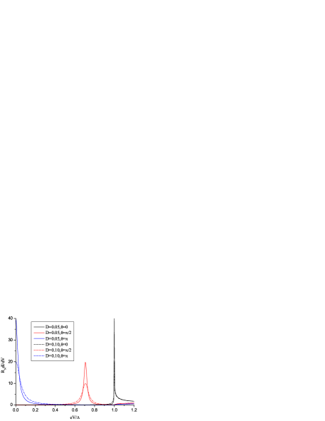
Figure 3: Differential conductance, $dI/dV$, for NFS contacts with different spin mixing angles, $\vartheta=0,\pi/2,\pi$ at $T=0$ and for $D_{\uparrow}=D_{\downarrow}\equiv D=0.05$ and $D=0.1$. The normal-state resistance of the point contact is $R_{N}=(e^{2}N_{f}D\,\mathcal{A})^{-1}$, where $\mathcal{A}$ is the area of the contact.

Asymmetry in the transmission probabilities, $D_{\uparrow}\neq D_{\downarrow}$, for spin up and spin down excitations also leads to a finite spin current. The corresponding spectral current density is given by

$$j^{s>}={2\left(D_{\uparrow}-D_{\downarrow}\right)\,\sinh(2\delta)\over e^{2\delta}+e^{-2\delta}R_{\uparrow}R_{\downarrow}-2\sqrt{R_{\uparrow}R_{\downarrow}}\cos\vartheta}\,,$$ (57)

for $|\epsilon|>\Delta$. In contrast to the charge current the sub-gap spin current spectral density vanishes identically ($j^{s<}=0$) because there is no resonant Andreev reflection for spin transport. The total spin current is then given by Eq. 56 with $j(\epsilon)\to j^{s}(\epsilon)$. In Fig. 4 we also show the differential spin conductance for weak spin filtering, $D_{\uparrow}=2D_{\downarrow}=0.2$. Note the onset of the spin conductance at $eV=\Delta$ for $T\to 0$, and the absence of Andreev resonance peaks in the spin conductance for non-zero spin mixing. The spin conductance is normalized by the normal-state spin conductance of a point contact of area $\mathcal{A}$, $(R^{s}_{N})^{-1}=N_{f}(D_{\uparrow}-D_{\downarrow})\,\mathcal{A}$.

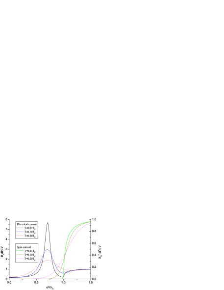
Figure 4: Differential charge conductance, $dI/dV$, and spin conductance, $dI^{s}/dV$, for an NFS contact with spin mixing angle, $\vartheta=\pi/2$ and transparencies, $D_{\uparrow}=2D_{\downarrow}=0.2$, at temperatures, $T=0.01T_{c}$, $T=0.1T_{c}$ and $T=0.2T_{c}$. Note that the voltage is normalized in units of $\Delta_{0}$, the gap at $T=0$.

The limit of extreme spin-filtering provided by a half-metallic ferromagnetic metal is discussed in detail using the transfer matrix method to incorporate spin-mixing at the interface between a FM and a superconductor.Kopu et al. (2004) We obtain the same results as Ref. Kopu et al., 2004 for the current of a half-metallic ferromagnetic-superconductor point contact by setting $D_{\uparrow}=D$ and $D_{\downarrow}=0$. In this limit the sub-gap conductance from resonant Andreev reflection is completely suppressed by the spin-filtering effect.

IV.2 SFS thermal conductance

In a recent report we discussed the role of Andreev bound states in regulating quasiparticle transport of heat through point-contact Josephson weak links.Zhao et al. (2003, 2004) Spin mixing generates a spin-resolved spectrum of Andreev bound states at a spin-active point contact even in the absence of a phase bias. We apply the formalism and boundary conditions developed in previous sections to investigate the effect of spin mixing on the phase sensitive heat transport in temperature biased SFS point contacts. We show that the relative phase shift of spin up and down electrons, together with the phase bias $\phi=\phi_{2}-\phi_{1}$, determines the spectrum of Andreev bound states at the point contact. The effects of these states on the transmission probability of continuum excitations that transport heat is calculated.

The thermal conductance of the point contact is defined by the ratio of the total heat current and the temperature bias $\delta T=T_{2}-T_{1}$ in the limit $\delta T\rightarrow 0$. The results reported below are normalized by the normal-state thermal conductance at $T_{c}$, $\kappa_{N}=\frac{\pi^{2}}{12}{\cal A}N_{f}v_{f}T_{c}(D_{\uparrow}+D_{\downarrow})$, where ${\cal A}$ is the area of the point contact.

Following the same line of argument as described for the NFS contact we apply the boundary conditions, Eqs. (6)-(25), to construct the Green functions for the SFS contact. The ABS spectrum is straightforward to calculate and has been discussed in the context of the Josephson current of the SFS weak link by several authors.M. Fogelström (2000); Cuevas and Fogelström (2001); Barash and Bobkova (2002) There are two branches (labelled as $\pm$) of spin-up Andreev bound states with energies,

$$\epsilon^{\uparrow}_{\pm}=\Delta\;\mathrm{sgn}\left(\sin{\vartheta\pm\rho\over 2}\right)\cos{\vartheta\pm\rho\over 2}\,,$$ (58)

where the angle $\rho$ is defined as

$$\rho=\arccos(\sqrt{R_{\uparrow}R_{\downarrow}}+\sqrt{D_{\uparrow}D_{\downarrow}}\cos{\phi})\,.$$ (59)

The spin down bound states are at energies

$$\epsilon^{\downarrow}_{\pm}(\vartheta)=\epsilon^{\uparrow}_{\pm}(-\vartheta)=-\epsilon^{\uparrow}_{\mp}(\vartheta)\,.$$ (60)

At $\vartheta=0$ or $\pi$, the ABS spectra is degenerate with respect to spin. For $0<\vartheta<\pi$ the spin degeneracy is lifted, thus, the typical bound state spectrum has four branches, two branches per spin direction for $\rho\neq 0$. Branches with opposite spin are “mirror reflections” of one another with respect to the Fermi energy ($\epsilon=0$). In the tunnelling limit, $D_{\uparrow}=D_{\downarrow}=D\rightarrow 0$, and to leading order in $\rho\ll\vartheta$, the splitting of the spin up states is given by

$$\epsilon^{\uparrow}_{\pm}\simeq\Delta[\cos{\vartheta\over 2}\mp\sin{\vartheta\over 2}\sqrt{D}\sin{\phi\over 2}]\,.$$ (61)

The spectral weight of an ABS comes at the expense of the continuum spectrum ($|\epsilon|>\Delta$). In addition there is asymmetry with respect to spin, $N^{\uparrow}(|\epsilon|>\Delta)\neq N^{\downarrow}(|\epsilon|>\Delta)$, and as a result spin up and spin down quasiparticles contribute differently to the heat current. To compute the heat current, we follow the procedure described in Ref. Zhao et al., 2003. The boundary conditions for the distribution functions, Eqs. (8) and (19), enable us to obtain an analytical result for the Keldysh Green’s function at the point contact. From this result we can calculate the spectral density for the heat current for the set of trajectories, $\{1i,1o,2i,2o\}$. The spectral heat current contains contributions from spin up and spin down electron-like and hole-like quasiparticles,

$$j^{h}(\epsilon,\hat{\mathbf{p}}_{f})={\epsilon\over 4\pi i}\mathrm{Tr}[\hat{g}^{K}_{1i}-\hat{g}^{K}_{1o}]={\epsilon\over 4\pi i}\mathrm{Tr}[\hat{g}^{K}_{2o}-\hat{g}^{K}_{2i}]\,,$$ (62)

where $\mathrm{Tr}$ represents the trace of Nambu matrix propagators. It is straightforward to show that the spectral heat current can be expressed in an intuitive form by introducing the effective transmission coefficient $\mathfrak{D}$ for heat transport,

$$j^{h}(\epsilon,\hat{\mathbf{p}}_{f})=-2\epsilon\left[\tanh{\epsilon\over 2T_{1}}-\tanh{\epsilon\over 2T_{2}}\right]\,\mathfrak{D}(\epsilon,\hat{p}_{f})\,.$$ (63)

The contributions to $\mathfrak{D}$ come from direct ($e\to e$) transmission and branch conversion ($e(h)\to h(e)$) transmission channels, $\mathfrak{D}=\mathfrak{D}_{e\to e}+\mathfrak{D}_{e\to h}$,

$$\mathfrak{D}_{e\to e} = [(D_{\uparrow}+D_{\downarrow})\cosh(2\delta)-2\sqrt{D_{\uparrow}D_{\downarrow}}\cos\vartheta\cos\phi)]$$ (64)

$$\times\sinh^{2}\delta/\mathcal{Z}^{2}$$

$$\mathfrak{D}_{e\to h} = [(D_{\uparrow}+D_{\downarrow})-2D_{\uparrow}D_{\downarrow}-2\sqrt{R_{\uparrow}R_{\downarrow}D_{\uparrow}D_{\downarrow}}\cos\phi]$$ (65)

$$\times\sinh^{2}\delta/\mathcal{Z}^{2}$$

$$\mathcal{Z}^{2} = [\sqrt{R_{\uparrow}R_{\downarrow}}+\sqrt{D_{\uparrow}D_{\downarrow}}\cos{\phi}-\cosh(2\delta)\cos\vartheta]^{2}$$ (66)

$$+\sinh^{2}(2\delta)\sin^{2}\vartheta\,.$$

In the normal state $\mathfrak{D}\to(D_{\uparrow}+D_{\downarrow})/2$, and spin mixing has no effect on the quasiparticle transport. However, in the superconducting state the transmission coefficient $\mathfrak{D}$ for quasiparticles of energy $\epsilon$ and momentum $\mathbf{p}_{f}$ is sensitive to both the phase bias, $\phi$, and the spin mixing angle, $\vartheta$.

Consider first the case with $\phi=0$. Spin mixing leads to bound states at $\epsilon_{\mathrm{B}}=\pm\Delta\cos(\vartheta/2)$. For the case in which $D_{\uparrow}=D_{\downarrow}=D$, only the direct transmission channel contributes, i.e. $\mathfrak{D}_{e\to h}(\phi=0)=0$ and

$$\mathfrak{D}_{e\to e}(\phi=0)=D{\epsilon^{2}-\Delta^{2}\over\epsilon^{2}-\Delta^{2}\cos^{2}{\vartheta\over 2}}<D\,.$$ (67)

Thus, quasiparticle transmission is suppressed by the spin mixing effect for any value of the normal-state transparency, $D$, and for all energies. The suppression is most severe at $\vartheta=\pi$, i.e. when the ABS is more strongly bound. Thus for $\phi=0$ spin mixing suppresses heat transport for any value of the normal state transparency.

For a spin-inactive point contact ($\vartheta=0$) in tunnelling limit, $D\ll 1$, it is known that $\mathfrak{D}(\epsilon)$ has a resonance peak at

$$\epsilon_{\mathrm{res}}/\Delta=1+{1\over 2}D\sin^{2}{\phi\over 2}+\mathcal{O}(D^{2})\,,$$ (68)

which is a reflection of a shallow bound state just below the gap edge at $\epsilon_{\mathrm{B}}/\Delta=1-{1\over 2}D\sin^{2}{\phi\over 2}+\mathcal{O}(D^{2})$. Tuning $\phi$ from 0 to $\pi$ leads to an increase in the thermal conductance because of resonant transmission of quasiparticles at $\epsilon\approx\epsilon_{\mathrm{res}}$.Zhao et al. (2003) Enhanced transmission still exists for SFS point contacts, but as $\vartheta$ increases the resonance peak of $\mathfrak{D}(\epsilon)$ gradually vanishes. For $\vartheta=\pi$, the bound states are at energies $\epsilon_{\mathrm{B}}=\pm\Delta\sqrt{D}\sin(\phi/2)$, and there is no resonance peak of $\mathfrak{D}(\epsilon)$. Instead $\mathfrak{D}$ is suppressed at all energies,

$$\mathfrak{D}(\vartheta=\pi)=D{\epsilon^{2}-\Delta^{2}\over\epsilon^{2}-\Delta^{2}D\sin^{2}{\phi\over 2}}<D\,.$$ (69)

Thus, to leading order in $D$, $\mathfrak{D}(\vartheta=\pi)\simeq D(1-\Delta^{2}/\epsilon^{2})$ is independent of $\phi$, so phase modulation of the thermal conductance vanishes. These features are shown clearly in Fig. 5 for the thermal conductance calculated in the tunnelling limit with $D_{\uparrow}=D_{\downarrow}=D=0.1$ and for general values of $\vartheta$ and $\phi$. Resonant enhancement of the conductance occurs in the vicinity of $\phi\approx\pi$ and $\vartheta\ll 1$. Increasing $\vartheta$ suppresses the overall thermal conductance as well as the phase modulation.

Figure 6 shows the thermal conductance in the high transparency limit with $D_{\uparrow}=D_{\downarrow}=D=0.9$. At $\vartheta=0$ (a “0” junction), tuning $\phi$ towards $\pi$ pushes the ABS deep into the gap, so $\mathfrak{D}(\epsilon)$ is increasingly suppressed from $D$, and the thermal conductance goes down. The opposite occurs at $\vartheta=\pi$ (a “$\pi$” junction M. Fogelström (2000)): tuning $\phi$ from 0 to $\pi$ pushes the ABS toward the gap edge, so the thermal conductance increases. The phase modulation of the thermal conductance for a general value of $\vartheta$ can be understood qualitatively in a similar manner. The thermal conductance is maximum when the bound states are closest to the gap edge. The different phase modulation of the thermal conductance for “0” junctions (i.e. $\vartheta<\pi/2$) versus “$\pi$” junctions ($\vartheta>\pi/2$) should be observable in high transparency SFS junctions; one should in principle be able to change the spin mixing angle by varying the thickness of the FM layer, thus tuning between “0” or “$\pi$” junction behavior. The phase of the SFS junction can then be controlled by varying the magnetic flux linking a SQUID containing the SFS contact.

In contrast to FM contacts, SFS junctions with FI contacts are expected to be in the tunnelling limit, i.e. $D_{\uparrow,\downarrow}\ll 1$. For the FI interface described in section III with $l=0.5$ nm, $D_{\uparrow}=0.013$, $D_{\downarrow}=0.007$ and $\vartheta=0.032\pi$, the discrimination between transparencies for different spin orientation is relatively large, $D_{\uparrow}\simeq 2D_{\downarrow}$, but the spin mixing is weak. As a result the phase modulation of the thermal conductance is almost the same as that of a spin-inactive tunnel junction.Zhao et al. (2003) Figure 7 shows a map of the thermal conductance as a function of temperature and phase bias for the junction parameters given above. For simplicity we neglected the angular dependence of $D_{\alpha}$ and $\vartheta$. Note that resonant transmission leads to enhancement of the thermal conductance compared to the normal-state conductance at $T_{c}$ over a broad temperature range $0.5T_{c}\lesssim T<T_{c}$ for $\phi\gtrsim\pi/2$.

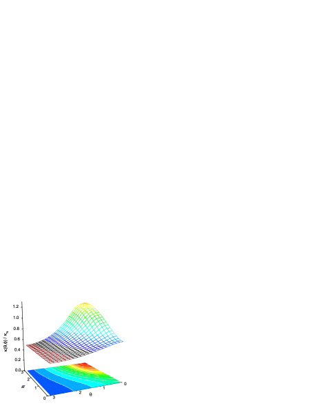
Figure 5: The thermal conductance of an SFS point contact with $D_{\uparrow}=D_{\downarrow}=0.1$ at $T=0.8T_{c}$. The thermal conductance is normalized to its value at $T_{c}$. $\phi$ and $\vartheta$ change from 0 to $\pi$.

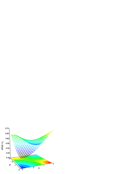
Figure 6: The thermal conductance for an SFS point contact with $D_{\uparrow}=D_{\downarrow}=0.9$ at $T=0.8T_{c}$.

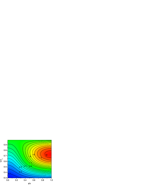
Figure 7: The thermal conductance of an SFS contact in the tunnelling limit with $D_{\uparrow}=2D_{\downarrow}=0.0013$ and $\vartheta\simeq 0.032\pi$.

V Discussion and Conclusion

In this paper we derived the boundary conditions for the quasiclassical Ricatti amplitudes, including the distribution functions, $x^{K}$, for general interfaces. This completes the development of the boundary conditions for the Riccati amplitudes at spin-active interfaces initiated in Refs. M. Fogelström, 2000. The results summarized in section II apply to a broad range of superconducting interfaces, and are specifically applicable to non-equilibrium transport involving spin-active interfaces. The boundary conditions can be applied to investigate dynamical properties, are applicable for any paring symmetry. The effects of disorder are readily described within the quasiclassical theory framework.

In the dirty limit the quasiclassical theory for conventional superconductors can be formulated in terms of Fermi surface averaged quasiclassical Green functions.Usadel (1970) The quasiclassical transport equations reduce to diffusion-type (Usadel) equations. Boundary conditions for the the Fermi-surface averaged Usadel propagators at a spin active interface has been discussed recently in Ref. Huertas-Hernando et al., 2002. A comparison between results for the dirty SFS and NFS junctions based on the Usadel equations and boundary conditions and the dirty limit of the Ricatti formalism with the general spin-active boundary conditions developed here will be discussed in a separate report. Finally, we note that we have presented boundary conditions and results applicable to specular interfaces. The boundary conditions can be extended to include atomic scale roughness at a spin-active interface, but this extension is outside the scope of this report.

The Riccati approach to the boundary problem in quasiclassical theory is complimentary to the T-matrix approach,Serene and Rainer (1983); Kieselmann (1985); Cuevas and Fogelström (2001); Eschrig et al. (2003); Kopu et al. (2004) which has been used to calculate the sub-harmonic structure of the current-voltage characteristics of magnetic Josephson point contacts,Andersson et al. (2002) and recently to study the Josephson effect and conductance of superconductors in contact with half-metallic ferromagnets.Eschrig et al. (2003); Kopu et al. (2004) The advantage of the Ricatti approach is that the implementation of the boundary condition is given explicitly in one step, without introducing auxiliary propagators. The Riccati formulation also makes analytical analysis more tractable. The Riccati method has been successfully used to study the equilibrium properties, e.g. the d.c. Josephson effect and temperature-induced $0-\pi$ transition of SFS junctions.M. Fogelström (2000); Barash and Bobkova (2002) As shown by Barash et al,Barash et al. (2002) the Riccati approach is especially powerful to study more complicated hybrid structures such as SFIFS junctions.

As examples of the potential application of the newly derived boundary condition for the non-equilibrium distribution functions, $x^{K}$, we investigated the charge and spin conductances for NFS point contacts and heat transport through temperature and phase biased SFS point contacts. We showed how the spin-mixing angle $\vartheta$, defined as the relative phase between spin up and down electrons upon transmission (or reflection), controls the local excitation spectrum and the transport of charge, spin, and energy across the point contact. Beyond this relatively simple application, we expect that new results and novel physics can be explored for a broad range of non-equilibrium transport problems involving spin-active interfaces with the new boundary conditions.

*

Appendix A Derivation of Eqs. (6)-(25)

In this appendix we outline how the boundary conditions for the Riccati amplitudes, Eq. (6)-(25), are derived from the Millis-Rainer-Sauls boundary conditions. Our starting point is the set of Eqs. (63)-(66) of Ref. Millis et al., 1988, which in terms of Shelankov projection operators,Shelankov (1985)

$$\check{P}^{\lambda}_{\pm}=\left(\begin{array}[]{cc}\hat{P}^{\lambda,R}_{\pm}&\hat{P}^{\lambda,K}_{\pm}\\ 0&\hat{P}^{\lambda,A}_{\pm}\end{array}\right)={1\over 2}(\check{1}\pm{\check{g}_{\lambda}\over-i\pi}),\lambda\in\{1i,1o,2i,2o\}$$ (70)

can be written as

$$\check{P}^{2o}_{-}(\hat{S}_{22}\check{P}^{2_{i}}_{+}\hat{S}^{\dagger}_{22}+\hat{S}_{21}\check{P}^{1i}_{-}\hat{S}^{\dagger}_{21})\check{P}^{2o}_{+}=0\,,$$ (71)

$$\check{P}^{2i}_{+}(\hat{S}^{\dagger}_{22}\check{P}^{2o}_{-}\hat{S}_{22}+\hat{S}^{\dagger}_{12}\check{P}^{1o}_{+}\hat{S}_{12})\check{P}^{2i}_{-}=0\,,$$ (72)

$$\check{P}^{1i}_{+}(\hat{S}^{\dagger}_{11}\check{P}^{1o}_{+}\hat{S}_{11}+\hat{S}^{\dagger}_{21}\check{P}^{2o}_{-}\hat{S}_{21})\check{P}^{1i}_{-}=0\,,$$ (73)

$$\check{P}^{1o}_{-}(\hat{S}_{11}\check{P}^{1i}_{-}\hat{S}^{\dagger}_{11}+\hat{S}_{12}\check{P}^{2i}_{+}\hat{S}^{\dagger}_{12})\check{P}^{1o}_{+}=0\,.$$ (74)

Following the convention in literature, we denote a Keldysh$\otimes$Nambu matrix with check accent, a Nambu (particle-hole$\otimes$spin) matrix with hat accent, and a spin matrix without any accent. We use the ansatz of EschrigEschrig (2000) to parameterize the projectors in terms of Riccati amplitudes, e.g. for $\check{P}_{+}^{1i}$ we have

$$\hat{P}^{R}_{+} = \left(\begin{array}[]{c}1\\ -\tilde{\Gamma}^{R}_{1}\end{array}\right)(1-\gamma^{R}_{1}\tilde{\Gamma}^{R}_{1})^{-1}(1,\;\gamma^{R}_{1})$$ (77)

$$\hat{P}^{A}_{+} = \left(\begin{array}[]{c}-\Gamma^{A}_{1}\\ 1\end{array}\right)(1-\tilde{\gamma}^{A}_{1}\Gamma^{A}_{1})^{-1}(\tilde{\gamma}^{A}_{1},\;1)$$ (80)

$$\hat{P}^{K}_{+} = \hat{P}^{R}_{+}\left(\begin{array}[]{cc}x^{K}_{1}&0\\ 0&0\end{array}\right)\hat{P}^{A}_{-}+\hat{P}^{R}_{-}\left(\begin{array}[]{cc}0&0\\ 0&\tilde{X}^{K}_{1}\end{array}\right)\hat{P}^{A}_{+}$$ (85)

where we omitted the superscript $1i$. The strategy to solve Eqs. (71)-(74) is to reduce the order of the equation set by exploiting the properties of the projectors and to decompose the equations for the Keldysh$\otimes$Nambu matrices into equations of spin matrices.

Take the retarded components of Eqs. (71)-(74) and plug in the expressions for $\hat{P}^{\lambda,R}_{\pm}$. Each of the four equations of Nambu matrices collapses into an equation for the coherence functions which are spin matrices. For example, the retarded part of Eq. (72) and (73) give

$$\beta^{R}_{12}(1-\Gamma^{R}_{1}\tilde{\gamma}^{R}_{1})^{-1}(\Gamma^{R}_{1}\underline{S}_{12}-S_{12}\gamma^{R}_{2})=(S^{\dagger}_{22}\Gamma^{R}_{2}-\gamma^{R}_{2}\underline{S}^{\dagger}_{22})(1-\tilde{\gamma}^{R}_{2}\Gamma^{R}_{2})^{-1}\tilde{\beta}^{R}_{22},$$ (86)

$$\beta^{R}_{11}(1-\Gamma^{R}_{1}\tilde{\gamma}^{R}_{1})^{-1}(\Gamma^{R}_{1}\underline{S}_{11}-S_{11}\gamma^{R}_{1})=(S^{\dagger}_{21}\Gamma^{R}_{2}-\gamma^{R}_{1}\underline{S}^{\dagger}_{21})(1-\tilde{\gamma}^{R}_{2}\Gamma^{R}_{2})^{-1}\tilde{\beta}^{R}_{12}.$$ (87)

Eqs. (86) and (87) suggest the solution

$$(\Gamma^{R}_{1}\underline{S}_{11}-S_{11}\gamma^{R}_{1})(\tilde{\beta}^{R}_{12})^{-1}=(\Gamma^{R}_{1}\underline{S}_{12}-S_{12}\gamma^{R}_{2})(\tilde{\beta}^{R}_{22})^{-1},$$ (88)

$$(\beta^{R}_{11})^{-1}(S^{\dagger}_{21}\Gamma^{R}_{2}-\gamma^{R}_{1}\underline{S}^{\dagger}_{21})=(\beta^{R}_{12})^{-1}(S^{\dagger}_{22}\Gamma^{R}_{2}-\gamma^{R}_{2}\underline{S}^{\dagger}_{22}).$$ (89)

The above results assume the inverses of $\beta^{R/A}_{ij}$ and their $\,\tilde{}$ partners exist. This is generally the case for partially transmitting interfaces. Otherwise, Eqs. (86) and (87) can be solved rather trivially since some of the $\mathcal{S}$ matrix elements vanish. Equations (88)-(89) immediately lead to the result obtained by Fogelström,M. Fogelström (2000) Eq. (26), which is equivalent to Eq. (6), as well as

$$\Gamma^{R}_{2} = r^{R}_{2l}\gamma^{R}_{2}\underline{S}^{\dagger}_{22}+t^{R}_{2l}\gamma^{R}_{1}\underline{S}^{\dagger}_{21}$$ (90)

$$r^{R}_{2l} = +[(\beta^{R}_{12})^{-1}S^{\dagger}_{22}-(\beta^{R}_{11})^{-1}S^{\dagger}_{21}]^{-1}(\beta^{R}_{12})^{-1}$$ (91)

$$t^{R}_{2l} = -[(\beta^{R}_{12})^{-1}S^{\dagger}_{22}-(\beta^{R}_{11})^{-1}S^{\dagger}_{21}]^{-1}(\beta^{R}_{11})^{-1}\,.$$ (92)

It is also straightforward to verify that the solution, Eq. (26) and Eqs. (90-92), indeed satisfy Eqs. (86) and (87). In a similar manner, the boundary conditions for all retarded and advanced coherence functions can be derived.

The Keldysh components of Eqs. (71)-(74) can be simplified by using the equations for retarded and advanced projectors. Then after plugging in the expressions for all the projectors, $\hat{P}^{\lambda,R/A/K}_{\pm}$, once again we find that the Nambu matrix equations collapse into spin matrix equations for the Riccati amplitudes. For example, the Keldysh components of Eqs. (72) and (73) lead to

$$0= [-\beta^{R}_{11}(1-\Gamma^{R}_{1}\tilde{\gamma}^{R}_{1})^{-1}S_{11}+(S^{\dagger}_{21}\Gamma^{R}_{2}-\gamma^{R}_{1}\underline{S}^{\dagger}_{21})(1-\tilde{\gamma}^{R}_{2}\Gamma^{R}_{2})^{-1}\tilde{\gamma}^{R}_{2}S_{21}]\;x^{K}_{1}$$ (93)

$$+x^{K}_{1}\;[-S^{\dagger}_{11}\gamma^{A}_{1}(1-\tilde{\Gamma}^{A}_{1}\gamma^{A}_{1})^{-1}(\tilde{\Gamma}^{A}_{1}S_{11}-\underline{S}_{11}\tilde{\gamma}^{A}_{1})+S^{\dagger}_{21}(1-\gamma^{A}_{2}\tilde{\Gamma}^{A}_{2})^{-1}\alpha^{A}_{21}]$$

$$+\beta^{R}_{11}(1-\Gamma^{R}_{1}\tilde{\gamma}^{R}_{1})^{-1}\;X^{K}_{1}\;(1-\gamma^{A}_{1}\tilde{\Gamma}^{A}_{1})^{-1}\alpha^{A}_{11}$$

$$-\beta^{R}_{21}(1-\Gamma^{R}_{2}\tilde{\gamma}^{R}_{2})^{-1}\;X^{K}_{2}\;(1-\gamma^{A}_{2}\tilde{\Gamma}^{A}_{2})^{-1}\alpha^{A}_{21}$$

$$-(S^{\dagger}_{11}\Gamma^{R}_{1}-\gamma^{R}_{1}\underline{S}^{\dagger}_{11})(1-\tilde{\gamma}^{R}_{1}\Gamma^{R}_{1})^{-1}\;\tilde{x}^{K}_{1}\;(1-\tilde{\Gamma}^{A}_{1}\gamma^{A}_{1})^{-1}(\tilde{\Gamma}^{A}_{1}S_{11}-\underline{S}_{11}\tilde{\gamma}^{A}_{1})$$

$$+(S^{\dagger}_{21}\Gamma^{R}_{2}-\gamma^{R}_{1}\underline{S}^{\dagger}_{21})(1-\tilde{\gamma}^{R}_{2}\Gamma^{R}_{2})^{-1}\;\tilde{x}^{K}_{2}\;(1-\tilde{\Gamma}^{A}_{2}\gamma^{A}_{2})^{-1}(\tilde{\Gamma}^{A}_{2}S_{21}-\underline{S}_{21}\tilde{\gamma}^{A}_{1}),$$

$$0= [-\beta^{R}_{12}(1-\Gamma^{R}_{1}\tilde{\gamma}^{R}_{1})^{-1}S_{12}+(S^{\dagger}_{22}\Gamma^{R}_{2}-\gamma^{R}_{2}\underline{S}^{\dagger}_{22})(1-\tilde{\gamma}^{R}_{2}\Gamma^{R}_{2})^{-1}\tilde{\gamma}^{R}_{2}S_{22}]\;x^{K}_{2}$$ (94)

$$+x^{K}_{2}\;[-S^{\dagger}_{12}\gamma^{A}_{1}(1-\tilde{\Gamma}^{A}_{1}\gamma^{A}_{1})^{-1}(\tilde{\Gamma}^{A}_{1}S_{12}-\underline{S}_{12}\tilde{\gamma}^{A}_{2})+S^{\dagger}_{22}(1-\gamma^{A}_{2}\tilde{\Gamma}^{A}_{2})^{-1}\alpha^{A}_{22}]$$

$$+\beta^{R}_{12}(1-\Gamma^{R}_{1}\tilde{\gamma}^{R}_{1})^{-1}\;X^{K}_{1}\;(1-\gamma^{A}_{1}\tilde{\Gamma}^{A}_{1})^{-1}\alpha^{A}_{12}$$

$$-\beta^{R}_{22}(1-\Gamma^{R}_{2}\tilde{\gamma}^{R}_{2})^{-1}\;X^{K}_{2}\;(1-\gamma^{A}_{2}\tilde{\Gamma}^{A}_{2})^{-1}\alpha^{A}_{22}$$

$$-(S^{\dagger}_{12}\Gamma^{R}_{1}-\gamma^{R}_{2}\underline{S}^{\dagger}_{12})(1-\tilde{\gamma}^{R}_{1}\Gamma^{R}_{1})^{-1}\;\tilde{x}^{K}_{1}\;(1-\tilde{\Gamma}^{A}_{1}\gamma^{A}_{1})^{-1}(\tilde{\Gamma}^{A}_{1}S_{12}-\underline{S}_{12}\tilde{\gamma}^{A}_{2})$$

$$+(S^{\dagger}_{22}\Gamma^{R}_{2}-\gamma^{R}_{2}\underline{S}^{\dagger}_{22})(1-\tilde{\gamma}^{R}_{2}\Gamma^{R}_{2})^{-1}\;\tilde{x}^{K}_{2}\;(1-\tilde{\Gamma}^{A}_{2}\gamma^{A}_{2})^{-1}(\tilde{\Gamma}^{A}_{2}S_{22}-\underline{S}_{22}\tilde{\gamma}^{A}_{2}).$$

Again, if the inverses of $\beta^{R/A}_{ij}$ do not exist Eqs. (93) and (94) simplify and are readily solved. For the general case, in order to solve for $X^{K}_{1}$ and $X^{K}_{2}$, we construct $(\beta^{R}_{21})^{-1}\times(Eq.\,\ref{XX1})\times(\alpha^{A}_{21})^{-1}-(\beta^{R}_{22})^{-1}\times(Eq.\,\ref{XX2})\times(\alpha^{A}_{22})^{-1}$ and $(\beta^{R}_{11})^{-1}\times(Eq.\,\ref{XX1})\times(\alpha^{A}_{11})^{-1}-(\beta^{R}_{12})^{-1}\times(Eq.\,\ref{XX2})\times(\alpha^{A}_{12})^{-1}$ to obtain transformed equations, Eq. (A.10)^′ and Eq. (A.11)^′, which are not reproduced here. The transformed Eq. (A.10)^′ contains only $X^{K}_{1},x^{K}_{1},x^{K}_{2}$ and $\tilde{x}^{K}_{2}$. We regularize each term by carrying out a series of transformations. For example, the terms proportional to $x^{K}_{1}$ are transformed to

$$+ (\beta^{R}_{21})^{-1}\beta^{R}_{11}(1-\Gamma^{R}_{1}\tilde{\gamma}^{R}_{1})^{-1}(a^{R}_{1l}\;\tilde{\gamma}^{R}_{2}S_{21}-S_{11})\;x^{K}_{1}\;(\alpha^{A}_{21})^{-1}+(\beta^{R}_{21})^{-1}\;x^{K}_{1}\;(S^{\dagger}_{21}\gamma^{A}_{2}\;\tilde{a}^{A}_{1r}-S^{\dagger}_{11})(1-\gamma^{A}_{1}\tilde{\Gamma}^{A}_{1})^{-1}\alpha^{A}_{11}(\alpha^{A}_{21})^{-1}$$ (95)

$$+ (\beta^{R}_{21})^{-1}\;x^{K}_{1}\;(\alpha^{A}_{21})^{-1}\,,$$

and further into

$$- (\beta^{R}_{21})^{-1}\beta^{R}_{11}(1-\Gamma^{R}_{1}\tilde{\gamma}^{R}_{1})^{-1}r^{R}_{1l}(S^{\dagger}_{11})^{-1}x_{1}(S_{11})^{-1}\tilde{r}^{A}_{1r}(1-\gamma^{A}_{1}\tilde{\Gamma}^{A}_{1})^{-1}\alpha^{A}_{11}(\alpha^{A}_{21})^{-1}$$ (96)

$$+ (\beta^{R}_{22})^{-1}\beta^{R}_{12}(1-\Gamma^{R}_{1}\tilde{\gamma}^{R}_{1})^{-1}r^{R}_{1l}(S^{\dagger}_{11})^{-1}x_{1}(S_{11})^{-1}\tilde{r}^{A}_{1r}(1-\gamma^{A}_{1}\tilde{\Gamma}^{A}_{1})^{-1}\alpha^{A}_{12}(\alpha^{A}_{22})^{-1}\,,$$

with the help of algebraic identities such as

$$a^{R}_{1l}\;\tilde{\gamma}^{R}_{2}S_{21}+r^{R}_{1l}=S_{11},\;a^{R}_{1l}\;\tilde{\gamma}^{R}_{2}S_{22}+t^{R}_{1l}=S_{12},$$ (97)

$$1-\Gamma^{R}_{1}\tilde{\gamma}^{R}_{1}=r^{R}_{1l}\beta^{R}_{11}+t^{R}_{1l}\beta^{R}_{12},$$ (98)

$$(\beta^{R}_{21})^{-1}\beta^{R}_{11}(1-\Gamma^{R}_{1}\tilde{\gamma}^{R}_{1})^{-1}t^{R}_{1l}\beta^{R}_{12}=(\beta^{R}_{22})^{-1}\beta^{R}_{12}(1-\Gamma^{R}_{1}\tilde{\gamma}^{R}_{1})^{-1}r^{R}_{1l}(\beta^{R}_{11})\,.$$ (99)

As a result the transformed Eqs. (A.10)^′ and (A.11)^′ can be expressed as

$$(\beta^{R}_{21})^{-1}\beta^{R}_{11}(1-\Gamma^{R}_{1}\tilde{\gamma}^{R}_{1})^{-1}n_{1}(1-\gamma^{A}_{1}\tilde{\Gamma}^{A}_{1})^{-1}\beta^{A}_{11}(\beta^{A}_{21})^{-1}=(\beta^{R}_{22})^{-1}\beta^{R}_{12}(1-\Gamma^{R}_{1}\tilde{\gamma}^{R}_{1})^{-1}n_{1}(1-\gamma^{A}_{1}\tilde{\Gamma}^{A}_{1})^{-1}\beta^{A}_{12}(\beta^{A}_{22})^{-1},$$ (100)

$$(\beta^{R}_{12})^{-1}\beta^{R}_{22}(1-\Gamma^{R}_{2}\tilde{\gamma}^{R}_{2})^{-1}n_{2}(1-\gamma^{A}_{2}\tilde{\Gamma}^{A}_{2})^{-1}\beta^{A}_{22}(\beta^{A}_{21})^{-1}=(\beta^{R}_{11})^{-1}\beta^{R}_{21}(1-\Gamma^{R}_{2}\tilde{\gamma}^{R}_{2})^{-1}n_{2}(1-\gamma^{A}_{2}\tilde{\Gamma}^{A}_{2})^{-1}\beta^{A}_{21}(\beta^{A}_{11})^{-1},$$ (101)

with

$$n_{1}\equiv X^{K}_{1}-r^{R}_{1l}x^{K}_{1}\tilde{r}^{A}_{1r}-t^{R}_{1l}x^{K}_{2}\tilde{t}^{A}_{1r}+a^{R}_{1l}\tilde{x}^{K}_{2}\tilde{a}^{A}_{1r}\,,$$ (102)

$$n_{2}\equiv X^{K}_{2}-r^{R}_{2l}x^{K}_{2}\tilde{r}^{A}_{2r}-t^{R}_{2l}x^{K}_{1}\tilde{t}^{A}_{2r}+a^{R}_{2l}\tilde{x}^{K}_{1}\tilde{a}^{A}_{2r}\,.$$ (103)

Obviously $n_{1}=n_{2}=0$ satisfies Eq. (100) and (101), or equivalently, the original Eqs. (93) and (94). The equation $n_{1}=0$ yields the boundary condition for $X^{K}_{1}$ in Eq. (8). The boundary condition for $\tilde{X}^{K}_{j}$ is derived in a similar manner starting from Eqs. (71) and (74).

References

- Wolf et al. (2001) S. A. Wolf, D. D. Awschalom, R. A. Buhrman, J. M. Daughton, S. von Molnár, M. L. Roukes, A. Y. Chtchelkanova, and D. M. Treger, Science 294, 1488 (2001).
- Tedrow and Meservey (1994) P. M. Tedrow and R. Meservey, Phys. Rep. 238, 173 (1994).
- Soulen et al. (1998) R. J. Soulen, J. M. Byers, M. S. Osofsky, B. Nadgorny, T. Ambrose, S. F. Cheng, P. R. Broussard, C. T. Tanaka, J. Nowak, J. S. Moodera, et al., Science 282, 85 (1998).
- Buzdin et al. (1982) A. Buzdin, L. Bulaevski, and S. Panyukov, 35, 147 (1982), [JETP Lett. 35, 178 (1982)].
- Buzdin and Kupriyanov (1991) A. Buzdin and M. Y. Kupriyanov, 53, 308 (1991), [JETP Lett. 53, 321 (1991)].
- Ryazanov et al. (2001) V. Ryazanov, V. Oboznov, A. Rusanov, A. Veretennikov, A. Golubov, and J. Aarts, Phys. Rev. Lett. 86, 2427 (2001).
- Kontos et al. (2002) T. Kontos, M. Aprili, J. Lesueur, F. Genet, B. Stephanidis, and R. Boursier, Phys. Rev. Lett. 89, 137007 (2002).
- Guichard et al. (2003) W. Guichard, M. Aprili, O. Bourgeois, T. Kontos, J. Lesueur, and P. Gandit, Phys. Rev. Lett. 90, 167001 (2003).
- M. Fogelström (2000) M. Fogelström, Phys. Rev. B 62, 11812 (2000).
- Barash and Bobkova (2002) Y. S. Barash and I. V. Bobkova, Phys. Rev. B 65, 144502 (2002).
- Koshina and Krivoruchko (2001) E. Koshina and V. Krivoruchko, Phys. Rev. B 63, 224515 (2001).
- Bergeret et al. (2001) F. S. Bergeret, A. F. Volkov, and K. B. Efetov, Phys. Rev. Lett. 86, 3140 (2001).
- Golubov et al. (2002) A. A. Golubov, M. Y. Kupriyanov, and Y. V. Fominov, Sov. Phys. JETP Lett. 75, 190 (2002).
- Barash et al. (2002) Y. S. Barash, I. V. Bobkova, and T. Kopp, Phys. Rev. B 66, 140503 (R) (2002).
- Blatter et al. (2001) G. Blatter, V. B. Geshkenbein, and L. B. Ioffe, Phys. Rev. B 63, 174511 (2001).
- Andersson et al. (2002) M. Andersson, J. C. Cuevas, and M. Fogelström, Physica C 367 (2002).
- Eliashberg (1972) G. M. Eliashberg, Sov. Phys. JETP 34, 668 (1972).
- Larkin and Ovchinnikov (1976) A. Larkin and Y. Ovchinnikov, Sov. Phys. JETP 41, 960 (1976).
- Serene and Rainer (1983) J. W. Serene and D. Rainer, Phys. Rep. 101, 221 (1983).
- Rammer and Smith (1986) J. Rammer and H. Smith, Rev. Mod. Phys. 58, 323 (1986).
- Kieselmann (1985) G. Kieselmann, Ph.D. thesis, Bayreuth Universität (1985).
- Cuevas and Fogelström (2001) I. C. Cuevas and M. Fogelström, Phys. Rev. B 64, 104502 (2001).
- Eschrig et al. (2003) M. Eschrig, J. Kopu, J. C. Cuevas, and G. Schön, Phys. Rev. Lett. 90, 137003 (2003).
- Kopu et al. (2004) J. Kopu, M. Eschrig, J. C. Cuevas, and M. Fogelström, Phys. Rev. B 69, 094501 (2004).
- Zaĭtsev (1984) A. V. Zaĭtsev, Sov. Phys. JETP 59, 1015 (1984), [Zh. Eskp. Teor. Fiz. 59, 1015 (1984)].
- Millis et al. (1988) A. Millis, D. Rainer, and J. A. Sauls, Phys. Rev. B38, 4504 (1988).
- Eschrig (2000) M. Eschrig, Phys. Rev. B 61, 9061 (2000).
- Schopohl and Maki (1995) N. Schopohl and K. Maki, Physica B 204, 214 (1995).
- Schopohl (1996) N. Schopohl, in Quasiclassical Methods in Superconductivity and Superfluidity, edited by D. Rainer and J. A. Sauls (1996), pp. 88–103, http://lanl.arxiv.org/abs/cond-mat/9804064.
- Eschrig et al. (1999) M. Eschrig, J. A. Sauls, and D. Rainer, Phys. Rev. B 60, 10447 (1999).
- Shelankov and Ozana (2000) A. Shelankov and M. Ozana, Phys. Rev. B 61, 7077 (2000).
- Tokuyasu et al. (1988) T. Tokuyasu, J. A. Sauls, and D. Rainer, Phys. Rev. B38, 8823 (1988).
- Zhao et al. (2003) E. Zhao, T. Löfwander, and J. A. Sauls, Phys. Rev. Lett. 91, 077003 (2003).
- Shiba (1968) H. Shiba, Prog. Theor. Phys. 40, 435 (1968).
- Löfwander et al. (2002) T. Löfwander, V. S. Shumeiko, and G. Wendin, Physica C 367, 86 (2002).
- Zhao et al. (2004) E. Zhao, T. Löfwander, and J. A. Sauls, Phys. Rev. B 69, 14 (2004).
- Usadel (1970) K. Usadel, Phys. Rev. Lett. 25, 507 (1970).
- Huertas-Hernando et al. (2002) D. Huertas-Hernando, Y. V. Nazarov, and W. Belzig, Phys. Rev. Lett. 88, 047003 (2002).
- Shelankov (1985) A. Shelankov, J. Low Temp. Phys. 60, 29 (1985).
- Hao et al. (1990) X. Hao, J. S. Moodera, and R. Meservey, Phys. Rev. B 42, 29 (1990).