Nonequilibrium steady states of the isotropic classical magnet

Abstract

We drive a $d$-dimensional Heisenberg magnet using a spatially anisotropic current of mobile particles or heat. The continuum Langevin equation is analyzed using a dynamical renormalization group, stability analysis and numerical simulations. We discover a rich steady-state phase diagram, including a critical point in a new nonequilibrium universality class, and a spatiotemporally chaotic phase. The latter may be ‘controlled’ in a robust manner to target spatially periodic steady states with helical order. We discuss several physical realizations of this model and make definite predictions which could be tested in experimental or model lattice systems.

I Introduction

There is a growing awareness that spatio-temporal chaos may be a generic feature of driven, dissipative, spatially extended systems with reversible terms in their equations of motion Das et al. (2002); Täuber et al. (2002, 1999) An understanding of this interplay between external drive, irreversible dissipation and reversible (inertial) dynamics may even be relevant to a deeper understanding of fluid turbulence described by the Navier Stokes equations. In light of this, a useful strategy is to construct simple spatially extended systems whose dynamics reveals this interplay Antal et al. (1999); Eisler et al. (2003) and study its consequences in a systematic manner. In an earlier shorter communication Das et al. (2002), we had successfully constructed such a driven, spatially extended system which, while ordered in the absence of the drive, inevitably enters a spatiotemporally chaotic state when driven. In this longer paper, in addition to providing analytical and numerical details of our earlier work, we present some new results and discuss several microscopic realizations of the dynamics. We hope this study will encourage searches for possible realizations in lattice models and, more important, experimental systems.

The simplest examples of driven, spatially extended systems is the class of models called driven diffusive lattice gas models (DDLG) Schmittmann and Zia (1995); Marro and Dickman (1999). While these models give rise to a variety of interesting dynamics, none of them is chaotic. Recall that the DDLG order parameter is Ising-like; its dynamics is therefore purely dissipative and externally driven and has no reversible (inertial) terms in the equation of motion. The simplest way to incorporate reversibility is to elevate the Ising to Heisenberg spins; the driven dynamics of the $O(3)$ Heisenberg spins has a natural precessional dynamics Ma and Mazenko (1975).

How do we drive the Heisenberg magnet spatio-temporally chaotic ? The dynamics of the classical Heisenberg magnet possesses several conserved quantities (in fact there are infinitely many in dimension $d=1$) Fogedby (13). One possibility is to destroy some of these conservation laws by driving it, not with an external field (which breaks the $O(3)$ symmetry explicitly) but by imposing a background steady current of heat or particles (or any other mobile species) which couples to the Heisenberg spins. If the dynamics of these mobile species is ‘fast’, then the imposed steady current may alter the effective dynamics of the isotropic magnet in a way so as to destroy some of the conservation laws of the un-driven system.

In fact, as we saw in Das et al. (2002), the classical $O(3)$ Heisenberg model in $d\equiv d_{\perp}+1$ dimensions Ma and Mazenko (1975) in the presence of a uniform current in one spatial direction (${\|}$), while retaining isotropy in the order parameter space, should be governed by the equations of motion

$$\frac{\partial{\vec{S}}}{\partial t} = \bigg{(}r_{\|}\partial_{\|}^{2}+r_{\perp}\nabla_{\perp}^{2}\bigg{)}{\vec{S}}-v{\vec{S}}-\frac{u}{6}({\vec{S}}\cdot{\vec{S}}){\vec{S}}-\lambda{\vec{S}}\times\partial_{\|}{\vec{S}}$$ (1)

$$+g_{\|}{\vec{S}}\times\partial_{\|}^{2}{\vec{S}}+g_{\perp}{\vec{S}}\times\nabla_{\perp}^{2}{\vec{S}}+\vec{\eta}\,.$$

Eq. (4) is a natural generalization of the DDLG models to the case of a 3-component axial-vector order parameter ${\vec{S}}$ and, as such, is an important step in the exploration of dynamic universality classes Hohenberg and Halperin (1977) far from equilibrium Täuber et al. (2002); Marculescu and Ruiz (1998). The local molecular field in which spins precess in this driven state is dominated by the nonequilibrium precession term involving $\lambda$, responsible for all the remarkable phenomena we predict, including a novel nonequilibrium critical point and, in a certain parameter range, a type of turbulence. Note that the noise $\vec{\eta}$ in our equations is a non-conserving scalar noise even though the dynamics of the Heisenberg model is spin-conserving in the absence of driving. We shall comment below on the origin of this non-conservation as well as that in the deterministic terms.

Here are our results : (i) Despite $O(3)$ invariance in the order-parameter space, the dynamics does not conserve magnetization; (ii) As a temperature-like parameter is lowered, the paramagnetic phase of the model approaches a nonequilibrium critical point in a new dynamic universality class controlled by the driving — we evaluate the dynamic $z$, roughening $\chi$ and anisotropy $\zeta$ exponents to leading order in $\epsilon=4-d$; (iii) Below this critical point, in mean-field theory without stochastic forcing, paramagnetism, ferromagnetism and helical order are all linearly unstable; (iv) Numerical studies in space dimension $d=1,2$, in the absence of stochastic forcing, show spatiotemporal chaos in this last regime. This chaos, when ‘controlled’, is replaced by spatially periodic steady helical states which are robust against noise.

We also discuss a variety of explicit lattice and continuum realizations of this long length scale dynamics with the hope that this will stimulate a search for experimental systems, e.g., isotropic magnets carrying a steady particle or heat current, as well as model magnetized lattice-gas simulations, where the predictions of our model can be tested. Our work reinforces the idea that spatiotemporal chaos is a generic feature of driven, dissipative, spatially extended systems with nonlinear reactive terms.

The generic occurrence of spatio-temporal chaos in this model is encouraging. It is instructive to compare this model with the dynamics of an incompressible fluid, embodied by the Navier-Stokes equations. Ignoring the fact that the while the total momentum of the fluid $\rho{\bf v}$ is conserved, the total spin in our model is not, the reader should not miss the formal similarity between the driven term ${\vec{S}}\times\partial_{\parallel}{\vec{S}}$ and the nonlinear $({\bf v}\cdot{\nabla}){\bf v}$ term in the Navier-Stokes, despite their disparate origins. The similarity of the convective nonlinearity of Navier-Stokes and the precession term in the dynamics of the classical Heisenberg model has already been remarked on Ma and Mazenko (1975); Forster et al. (16); the form of our drive term (bilinear with one gradient) makes this resemblance closer. Our equations are however more amenable to quantitative analysis, since, unlike Navier-Stokes, they are non-trivial even in $d=1$.

A section-wise breakup : In section II we provide a derivation of the equations of motion for the driven Heisenberg magnets (DHM) both from general symmetry arguments and by analyzing explicit magnetized lattice-gas and continuum models. We next analize the steady state phase diagram of the continuum equations of motion (Section III), and show that the ‘high drive-temperature’ steady state of the model is paramagnetic (Sect. IIIa). There exists a nonequilibrium critical point whose critical exponents are determined using a dynamical renormalization group calculation (Sect. IIIb). Lastly (Sect. IIIc) we study the ‘low drive-temperature’ phase of the system which exhibits spatio-temporal chaos. This chaotic phase may be ‘controlled’ giving rise to a steady state configuration with broken chiral symmetry (Section IV). We end with a discussion of results and future directions (Section V). The details of the diagrammatic calculations are relegated to an appendix (Appendix A).

II Dynamics of Driven Heisenberg Magnets

Consider a system of Heisenberg ($O(3)$) spins situated either on a (hypercubic) lattice or a continuum in $d$-dimensions. Imagine a current of mobile species moving along one spatial direction (say ${\hat{z}}$), and interacting with the $O(3)$ spins. The spins interact with their neighboring spins via an exchange interaction (or any other short-range ferromagnetic interaction). If we treat the mobile species as being ‘faster’ (in a way which we will make precise) than the spins, then we may ask for the effective dynamics of the Heisenberg spins themselves. We first derive the effective dynamics of the spins using general symmetry arguments and conservation laws. While such arguments are robust in themselves, they may not be realizable in a given physical setting. To counter this criticism we also construct explicit microscopic realizations of the DHM.

II.1 General Symmetry Arguments

In this section we explain, how to construct, on general grounds of symmetry, the leading terms in the equations of motion of a uniaxially driven Heisenberg magnet.

First let us remind ourselves of the equations of motion for spins at thermal equilibrium at temperature $T$. The probability of spin configurations $\{\vec{S}_{i}\}$ of a general nearest-neighbor Heisenberg chain with sites $i$ is $\propto\exp(-H/T)$, with an energy function

$$H=-\sum_{i}J_{i}\vec{S}_{i}\cdot\vec{S}_{i+1},$$ (2)

where $J_{i}$ is the ferromagnetic exchange coupling between $i$ and $i+1$. A spin $\vec{S}_{i}$ at $i$ precesses as $\dot{\vec{S}}_{i}=\vec{S}_{i}\times\vec{h}_{i}$ where

$$\vec{h}_{i}=-{\partial H\over\partial\vec{S}_{i}}=J_{i}\vec{S}_{i+1}+J_{i-1}\vec{S}_{i-1}$$ (3)

is the local molecular field. Replacing $J_{i}\to J(x)$ and $\vec{S}_{i}\to\vec{S}(x)$ in the continuum limit, yields Balakrishnan (1982) $\dot{\vec{S}}(x)=J(x)\vec{S}\times\partial^{2}_{x}\vec{S}+(dJ/dx)\vec{S}\times\partial_{x}\vec{S}+...$. For the physically reasonable case where $J$ varies periodically about a mean value $J_{0}$, this reduces for long wavelengths to $\dot{\vec{S}}(x)=J_{0}\vec{S}\times\partial^{2}_{x}\vec{S}$, which is invariant under $x\to-x$, even if the $H$ is not. If we impose a macroscopic distinction between $x$ and $-x$ in the form of an (admittedly artificial) $J$ varying linearly with $x$, say $J=ax$ where $a$ is a constant, we see that a term $a\vec{S}\times\partial_{x}\vec{S}$ arises. However, the other term so generated, namely, $J(x)\vec{S}\times\partial^{2}_{x}\vec{S}$, has a coefficient which grows with $x$, presenting problems in the limit of infinite system size. The dynamics in either of these cases conserves $\sum_{i}\vec{S}_{i}$ since it commutes with $H$. Note that we have so far insisted on a local field arising from an energy function as in (3).

Let us now ask what the most general equation of motion for $\vec{S}$ would be, if we relax the $x\to-x$ symmetry and no longer insist on an energy function. This would clearly be the appropriate approach if the system were carrying a steady drift current of some mobile species – particles, vacancies, heat – in, say, the ${\bf\hat{x}}$ direction, retaining isotropy in spin space. Let us not specify at this stage how these additional degrees of freedom couple to the spins. It is sufficient to note that, irrespective of the nature of such couplings, the spins will be in a nonequilibrium state so that their dynamics will not follow from an energy function, and must be constructed anew.

If we average over the degrees of freedom directly associated with the current (the mobile species are ‘faster’ than the spins), their effect should be simply to modify the equations for the $\vec{S}_{i}$ by allowing terms forbidden at thermal equilibrium. On general symmetry grounds the new terms will clearly involve an odd number of spatial derivatives. To lowest order in gradients, there are only two such terms: $v\partial_{x}{\vec{S}}$ and $\lambda{\vec{S}}\times\partial_{x}{\vec{S}}$. The first term, representing advection by a mean drift, may be eliminated by a Galilean transformation $x\to x+vt$, $t\to t$, leaving only the second term to reflect the drive. It is clear that the second term simply represents the continuum limit of asymmetric exchange, i.e., $\vec{h}_{i}=J_{+}\vec{S}_{i+1}+J_{-}\vec{S}_{i-1}$ with $\lambda\propto J_{+}-J_{-}$ proportional to the driving rate. Such a term would be ruled out Ma and Mazenko (1975) at thermal equilibrium only because the dynamics had to be generated by (2) and (3).

If we start with the usual Ma-Mazenko Ma and Mazenko (1975) dynamics for $\vec{S}$, with spin-conservation built in to both the systematic and noise terms, and then add in our novel precession ($\lambda$) term, then standard perturbation theory for the noise and propagator renormalization yields, already at one-loop order, non-conserving terms of the form $({\vec{S}}\cdot{\vec{S}})^{n}\,{\vec{S}}$ in the limit of zero external wavenumber even if these are not put in at the outset. This is because the $\lambda$ term, while rotation-invariant in spin space, is not the divergence of a current Kardar et al. (1986); NOT and, thus, does not conserve total spin. A renormalization-group theory of the long-wavelength dynamics of such a driven system must allow from the start for such nonconserving terms.

For a general dimension $d\equiv d_{\perp}+1$, with anisotropic driving along one direction (${\|}$) only, the above arguments yield, to leading orders in a gradient expansion, the generalized Langevin equation (which possesses spatial $O(d-1)$ symmetry),

$$\frac{\partial{\vec{S}}}{\partial t} = \bigg{(}r_{\|}\partial_{\|}^{2}+r_{\perp}\nabla_{\perp}^{2}\bigg{)}{\vec{S}}-v{\vec{S}}-\frac{u}{6}({\vec{S}}\cdot{\vec{S}}){\vec{S}}-\lambda{\vec{S}}\times\partial_{\|}{\vec{S}}$$ (4)

$$+g_{\|}{\vec{S}}\times\partial_{\|}^{2}{\vec{S}}+g_{\perp}{\vec{S}}\times\nabla_{\perp}^{2}{\vec{S}}+\vec{\eta}\,,$$

where we have allowed explicitly for spatial anisotropy in all coefficients. The Gaussian, zero-mean nonconserving noise $\vec{\eta}$ satisfies

$$\langle\eta_{\alpha}({\bf x},t)\eta_{\beta}({\bf x}^{\prime},t^{\prime})\rangle=2B\,\delta_{\alpha\beta}\,\delta^{d}({\bf x}-{\bf x}^{\prime})\delta(t-t^{\prime})\,.$$ (5)

Note that the noise in our equations is a non-conserving scalar noise. It is vectorial only in internal (spin) space but is a scalar under spatial rotations. The correlation function of such a noise, at zero wavenumber, cannot detect spatial anisotropy. If the noise were conserving, the covariance at wavevector ${\bf q}=(q_{||},{\bf q}_{\perp})$ would in general be proportional to $q_{||}^{2}+\alpha q_{\perp}^{2}$, for some constant $\alpha\neq 1$. Such additive, conserving but anisotropic contributions to the noise doubtless exist here as well, but are irrelevant at small wavenumber relative to the nonconserving noise.

Having established the form of the coarse-grained equations of motion on general symmetry grounds, we now offer explicit microscopic models within which the novel, nonequilibrium precession term could arise.

II.2 Construction of Explicit Examples

Recall that we are trying to create a driven state with directed spatial anisotropy (i.e., distinguishing, say, $x$ from $-x$) while retaining isotropy in the spin degrees of freedom. Clearly, this cannot be achieved by means of a steady imposed spin current, since that would pick out a spin direction. We suggest here some approaches to achieve this. (I) Impose a steady current in some other species through the material and to show that this leads, via symmetry-allowed couplings between this additional degree of freedom and the spins, to the nonequilibrium precession term. The dynamics for the additional species is conserving; there is, strictly, speaking, no timescale on which the additional variables can be treated as fast and eliminated to yield an effective equation of motion for the spins alone. We must therefore employ a driven variant of model D, in the language of Ref. Hohenberg and Halperin (1977). The effective spin dynamics we actually use in our paper should, however, apply in the limit of an infinitely large diffusivity for the additional species or if processes that violate the conservation law for the additional species can be made to intervene. (II) Introduce the driving as a fluctuating magnetic field, statistically isotropic in spin space, but with short-ranged correlations which distinguish $x$ from $-x$. In both these cases (and, it seems clear, in general) it turns out that the exchange couplings have to be dynamical, not constant, in order to generate the nonequilibrium precession term. We now examine each of these cases.

Consider a 1-dimensional lattice, each site $i$ of which can be either vacant ($n_{i}(t)=0$) or occupied by one particle ($n_{i}(t)=1$) at time $t$. Each particle has an attached Heisenberg spin and may hop to the nearest neighbor at the right (left), if vacant, with probability $p$ ($q$). The spin $\vec{S}_{i}(t)$ at an occupied site $i$ is the spin of the occupying particle. The local field at site $i$ is $\vec{h}_{i}(t)=J_{i-1,i}\vec{S}_{i-1}(t)+J_{i+1,i}\vec{S}_{i+1}(t)$ where the exchange coupling $J_{ij}(t)$ determines, at time $t$, the field at $j$ due to the spin at $i$. If we let $J_{ij}$ depend on the configuration of the ${n_{i}}$ as $J_{ij}(t)=n_{i}(t)n_{j}(t)[J_{1}+(J_{2}-J_{1})n_{j}(t-1)]$, with the ${n_{i}}$ governed by an asymmetric exclusion process (ASEP) Schmittmann and Zia (1995); Marro and Dickman (1999) the driving nonlinearity in (4) is generated naturally. Explicitly, $J_{i,i\pm 1}(t)=J_{1}$ or $J_{2}$ according as $n_{i}(t-1)=1$ or $0$, since the exchange coupling between, say, $i-1$ and $i$ is operative at time $t$ only if $n_{i-1}(t)n_{i}(t)=1$, Assume for simplicity that the particles can hop only to the right. Then a configuration $111$ at sites $i-1,\,i,\,{\rm and}\,i+1$ at time $t$ was either already present at time $t-1$ or arose from $011$ (by a right hop from $i-2$). Thus, for $111$ configurations, $J_{i-1,i}$ will be a weighted average of $J_{1}$ and $J_{2}$, while $J_{i+1,i}$ will be $J_{1}$. In the continuum limit, and averaging over the particle dynamics, we will get the driving term in (4), with $\lambda\propto p-q$.

The assumption of fast dynamics for the ASEP variable is justified if we allow evaporation-deposition as well, thus annulling the conservation law for particles. The derivation in our paper for the effective asymmetric exchange felt by a spin at a given site remains unaltered by this non-conservation since, unlike the hopping, the evaporation-deposition affects in an unbiased manner the sites on either side of the spin in question. Of course, particle non-conservation induces spin non-conservation trivially in this case.

More generally, let us construct a dynamical exchange coupling $J_{ij}(t)$ for a collection of spins in a host lattice which lacks invariance under $x\to-x$. Imagine that the system is in a nonequilibrium environment, stationary, isotropic and translation-invariant in a statistical sense, in the form of a fluctuating magnetic field $\vec{h}_{i}$ at every point $i$ of the lattice. Assume that $J_{ij}(t)$ has a piece $\Delta J_{ij}(t)\propto\vec{h}_{i}(t)\cdot\vec{h}_{j}(t-\tau)$ where $\tau$ is some timescale intrinsic to the material. Since the material lacks $x\to-x$ invariance, the average $\langle\Delta J_{ij}\rangle\propto\langle\vec{h}_{i}(t)\cdot\vec{h}_{j}(t-\tau)\rangle$ is in general nonsymmetric in $ij$ if the sites $i,j$ are separated in the $x$ direction. Microscopically, this could happen if there is some underlying dynamical process, for instance structural relaxation, determining the exchange couplings between sites $i$ and $j$. Note that we do not need explicitly to drive anything through the system; asymmetry under $x\to-x$ and a nonequilibrium noise should suffice to produce this ratchet-like effect. In addition, the precession of spins in this fluctuating field implies a term $\vec{S}_{i}\times\vec{h}_{i}$ which is not spin conserving.

Curiously, a term with precisely the form of our nonequilibrium precession term appears in the equilibrium dynamics of the staggered magnetization in the isotropic antiferromagnet, as presented in the work of Balakrishnan (1982). The consequences of such a term appear not to be very dramatic there, presumably because of the presence of other couplings to the ferromagnetic order parameter. In addition, equation (4) with no noise and with all coefficients on the right-hand side except $\lambda$ set to zero is known in the literature as the Belavin-Polyakov equation Belavin and Polyakov (1975); Rajaraman (1982) and has been widely studied for its soliton solutions.

Moving to a completely different description, consider the dynamics of chiral self-propelled particles Lau et al. (2003) described by a polar vector ${\vec{n}}$, suspended in a fluid and drifting along the ${\hat{z}}$ direction. A transient variation of $\vec{n}$ along ${\hat{z}}$ must lead Purcell (1977) to an overall rotation about $\vec{n}$. Shifting away the effect of the mean drift this clearly yields a dynamics of the form $\partial_{t}{\vec{n}}\sim{\vec{n}}\times\partial_{z}{\vec{n}}+\ldots\,\,$ which is once again our nonequilibrium precession term. The consequences of this for the dynamics of self-propelled chiral objects remain to be worked out.

II.3 Fokker Planck Equation and absence of an FDT

Since in the Langevin dynamics of this driven Heisenberg magnet, both the nonconservative noise and deterministic terms arise from the external drive, there is no obvious relation (such as the fluctuation-dissipation theorem (FDT)) between the variance of the nonconservative noise and dissipation Chaikin and Lubensky (1998). This may easily be seen by constructing the Fokker-Planck equation Kampen (1985) for the probability distribution of spins $P(\{{\vec{S}}\},t)$ corresponding to the Langevin equation (4),

$$\frac{\partial P}{\partial t}=-\frac{\partial}{\partial S_{\alpha}}\left[A_{\alpha}P-B\frac{\partial P}{\partial S_{\alpha}}\right]$$ (6)

where

$${\vec{A}} = \bigg{(}r_{\|}\partial_{\|}^{2}+r_{\perp}\nabla_{\perp}^{2}\bigg{)}{\vec{S}}-v{\vec{S}}-\frac{u}{6}({\vec{S}}\cdot{\vec{S}}){\vec{S}}-\lambda{\vec{S}}\times\partial_{\|}{\vec{S}}$$ (7)

$$+g_{\|}{\vec{S}}\times\partial_{\|}^{2}{\vec{S}}+g_{\perp}{\vec{S}}\times\nabla_{\perp}^{2}{\vec{S}}$$

Since the stationary probability distribution of the steady state configurations need not be the equilibrium canonical distribution $\exp(-F[{\vec{S}}]/T)$ at a temperature $T$ (where $F$ is the free-energy functional), there is no direct relation between the $B$ and the other parameters that enter the Langevin equation.

III Nonequilibrium Steady States

Having discussed several microscopic realizations of the coarse-grained continuum dynamics Eq. (4), we will proceed to establish a ‘nonequilibrium phase diagram’ of steady states obtained by analyzing the stationary solutions ($\partial_{t}{\vec{S}}=0$) of Eq. (4). Let us specify the parameters in our ‘phase diagram’.

In the equilibrium, isotropic limit, $\lambda=u=v\equiv 0$, $r_{\|}=r_{\perp}\equiv r$, the noise strength (which is conserved in the absence of the drive) vanishes at zero wavenumber, and Eq. (4) has a critical point where the renormalized $r$ goes to zero. In the driven state, the dynamics and noise are nonconserving; the critical point is at $v=0$, which in general takes place on a curve in the temperature/driving-force plane. As the drive is taken to zero there should be a crossover from nonequilibrium to equilibrium critical behavior. Our primary interest is in the behavior at a given nonzero driving rate, for which it suffices to vary the temperature-like parameter $v$ (which we shall refer to as ‘drive-temperature’) in (4), keeping the rest fixed (with $r_{\|},\,r_{\perp},u>0$). Note that the variance of the nonconserved noise $B$ is another temperature-like parameter. Since the FDT is violated by the external drive, these two temperature-like variables $v$ and $B$ are not related to each other. The nonequilibrium phase diagram will therefore be parametrized by the two parameters $v$ and $B$.

III.1 Dynamics at High Drive-Temperatures ($v>0$)

At high drive-temperatures the steady state, obtained by setting $\partial_{t}{\vec{S}}=0$ is paramagnetic, characterized by $\langle{\vec{S}}({\bf x},t)\rangle=0$ ($\langle\cdot\cdot\cdot\rangle$ denotes an average over the noise $\vec{\eta}$) and correlators . The effect of the drive is to change the correlation lengths $\xi_{\perp}=\sqrt{r_{\perp}/v}+O(\lambda^{2}/\sqrt{v})-O(\lambda^{2})$ and $\xi_{\|}=\sqrt{r_{\|}/v}+O(\lambda^{2}/\sqrt{v})-O(\lambda^{2})$. Thus for $v>0$ (the paramagnetic phase) all correlations clearly decay on finite lengthscales $\sim 1/\sqrt{v}$ and time-scales $\sim 1/v$, and nonlinearities are irrelevant. We find that this paramagnetic state is stable under dynamical perturbations. This can be seen by writing ${\vec{S}}({\bf x},t)=\langle{\vec{S}}({\bf x},t)\rangle+{\vec{u}}({\bf x},t)$, where ${\vec{u}}$ is an arbitrary small perturbation. The time evolution of ${\vec{u}}({\bf x},t)$ to linear order is given by

$$\frac{\partial{\vec{u}}}{\partial t}=\left(r_{\perp}\nabla^{2}_{\perp}+r_{\|}\partial^{2}_{\|}-v\right){\vec{u}}+\vec{\eta}\,,$$ (8)

which on Fourier transformation reads

$${\vec{u}}_{\bf k}(t) = {\vec{u}}_{\bf k}(0)\exp(-\gamma_{\bf k}t)$$ (9)

$$+\int_{0}^{\infty}dt^{\prime}\vec{\eta}_{\bf k}(t^{\prime})\exp(-\gamma_{\bf k}(t-t^{\prime}))\,,$$

where

$$\gamma_{\bf k}=r_{\perp}k^{2}_{\perp}+r_{\|}k^{2}_{\|}+v\,.$$ (10)

This arbitrary perturbation ${\vec{u}}_{\bf k}$ always decays to zero when $v>0$. The ‘paramagnetic phase’ is therefore linearly stable.

III.2 Dynamics in the Critical Phase $(v=0)$: New Critical Behavior

A description of the nature of correlations on the critical surface $v=0$, requires the machinery of the Dynamical Renormalization Group (DRG). While there are several clear expositions of this technique Medina et al. (1989) devised for specific problems, we hope that some readers may benefit from a pedagogical treatment of DRG applied to our anisotropic driven Heisenberg dynamics.

Let us first drop all nonlinear terms from the equations of motion. In the critical region, defined by $v=0$, the linear theory is massless resulting in divergent long wavelength fluctuations, as can be seen by explicitly calculating the correlation function $C(x,t)=\langle{\vec{S}}({\bf x}+{\bf x}^{{}^{\prime}},t+t^{{}^{\prime}})\cdot{\vec{S}}({\bf x}^{{}^{\prime}},t^{{}^{\prime}})\rangle$ from Eq. (4) when $u=\lambda=0$. The correlation function is easily recast as a scaling form,

$$C(x,t)=\frac{B}{r_{\|}}x_{\|}^{2\chi}F_{0}\bigg{(}\frac{r_{\|}t}{x_{\|}^{z}},\frac{x_{\perp}}{x_{\|}^{\zeta}}\sqrt{\frac{r_{\|}}{r_{\perp}}}\bigg{)}\,,$$ (11)

where the roughening exponent $\chi=1-d/2$, the growth exponent $z=2$, the anisotropy exponent $\zeta=1$, and $F_{0}$ is an analytic function of its arguments.

What is the nature of these divergent fluctuations in the presence of the nonlinear terms? This can be addressed via a standard implementation of the dynamical renormalization group (DRG) Medina et al. (1989) based on a perturbative expansion in the small couplings $\lambda$ and $u$, about the linear theory. The perturbative corrections to the correlation function may be equivalently viewed as arising from modifications (renormalization) of the parameters $r_{\|},\,r_{\perp}$ and $B$. Renormalizability guarantees that the correlation function $C(x,t)$ will retain a scaling form as in Eq. (11) with modified exponents $z$, $\zeta$, $\chi$ and a new scaling function

$$C(x,t)=x_{\|}^{2\chi}F\bigg{(}\frac{t}{x_{\|}^{z}},\frac{x_{\perp}}{x_{\|}^{\zeta}}\bigg{)}\,.$$ (12)

This implies that the critical region, defined by (renormalized) $v^{R}=0$, still has divergent long wavelength fluctuations. In what follows we assume renormalizability, which we justify post facto to lowest order in perturbation.

The perturbation expansion would make sense only if the couplings $\lambda$ and $u$ are small. This is ensured by the DRG procedure which involves a systematic expansion about the upper critical dimension $d_{c}$. As we shall see, the renormalized couplings $\lambda$ and $u$ will flow to small values, of order $\epsilon=d_{c}-d$. The upper critical dimension may be obtained by a simple power-counting argument. Rescale space, time and the order parameter as : $x_{\|}=bx_{\|}^{\prime},\,{\bf x}_{\perp}=b^{\zeta}{\bf x}_{\perp}^{\prime},\,t=b^{z}t^{\prime}$ and ${\vec{S}}=b^{\chi}{\vec{S}}^{\prime}$, where $b>1$ is an arbitrary parameter. We may reinterpret the effect of such a rescaling as a change in the parameters ; thus the form of Eq. (4) will remain unchanged if we change the parameters to their primed values $r^{\prime}_{\|}=b^{z-2}r_{\|}$, $r^{\prime}_{\perp}=b^{z-2\zeta}r_{\perp}$, $B^{\prime}=b^{z-2\chi-\zeta(d-1)-1}B$, $u^{\prime}=b^{4-d}u$, $\lambda^{{}^{\prime}}=b^{\chi+z-1}\lambda$, $g_{\|}^{{}^{\prime}}=b^{\chi+z-2}g_{\|}$, and $g_{\perp}^{{}^{\prime}}=b^{\chi+z-2}g_{\perp}$. Demanding that the linear equation (in the absence of nonlinearities, $u=\lambda=g_{\|}=g_{\perp}=0$) be scale invariant, automatically fixes $\chi=1-d/2$, $z=2$, $\zeta=1$, consistent with Eq. (11).

Inserting the values of the exponents evaluated within the linear theory, we find that the couplings $\lambda$ and $u$ are relevant, i.e., they grow under rescaling, for dimensions $d<d_{c}=4$, the upper critical dimension for these couplings. Thus nontrivial exponents are expected for $d<d_{c}=4$ in the presence of nonlinearities. The mean-field estimates in the previous paragraph are valid for $d\geq 4$. The other two couplings $g_{\|}$ and $g_{\perp}$ have an upper critical dimension $d_{c}^{g}=2$; they are therefore irrelevant for $d$ near $4$, and will be set to zero in the analysis that follows.

We now carry out the DRG calculation to compute the corrections to the new exponents and the scaling function due to the nonlinear terms using a field theoretic approach Medina et al. (1989); Amit (1978); Brezin et al. (1976); ’t Hooft and Veltman (1972). The DRG procedure involves, as usual, two steps —

(i) Start with a large-wavenumber cutoff $\Lambda$. Solve the equation of motion iteratively in an expansion in $u$ and $\lambda$ Average over modes with wavenumber $k$ in the shell $(\Lambda/b,\Lambda)$, with $b=e^{\ell}$, to obtain “intermediate” renormalized parameters $r_{\perp}^{I}$, $r_{\|}^{I}$, $\lambda^{I}$ etc. in the equations of motion. This averaging is carried out to leading order in $\lambda$ and $u$, justified post facto by the fact that these couplings flow to small values, of order $\epsilon$, at the DRG fixed point in dimension $d=4-\epsilon$. (ii) Rescale space, time, and fields as in the previous paragraph to restore the original cutoff $\Lambda$. The parameters $r_{\perp}^{I}$ etc. will then acquire rescaling factors as above. Define $r_{\perp}(\ell)\equiv b^{z-2\zeta}r_{\perp}^{I}$, and similarly define $\ell$-dependent versions of the other parameters in the equation. This may be recast as differential recursion equations in the various couplings.

(i)Perturbative Calculation : The bare (unrenormalized) propagator $G_{0}({\bf k},\omega)$ and the correlator $C_{0}({\bf k},\omega)$ are defined from the linear theory as

$$G_{0}({\bf k},\omega) = \frac{1}{r_{\|}k_{\|}^{2}+r_{\perp}k_{\perp}^{2}+v-i\omega}\,,$$

$$C_{0}({\bf k},\omega) = \langle{\vec{S}}({\bf k},\omega)\cdot{\vec{S}}(-{\bf k},-\omega)\rangle$$ (13)

$$= \frac{2B}{(r_{\|}k_{\|}^{2}+r_{\perp}k_{\perp}^{2}+v)^{2}+\omega^{2}}\,.$$

We next calculate the corrections to the correlation functions from the nonlinearities, perturbatively in the couplings $u$ and $\lambda$. On Fourier transforming Eq. (4) we obtain

$$S_{\alpha}({\bf k},\omega)=G_{0}({\bf k},\omega)\eta_{\alpha}-\frac{i\lambda}{2}G_{0}({\bf k},\omega)\int d^{-}qd^{-}\nu[q_{\|}-(k_{\|}-q_{\|})]\epsilon_{\alpha\beta\delta}S_{\beta}({\bf q},\nu)S_{\delta}({\bf k}-{\bf q},\omega-\nu)$$

$$-uF_{\alpha\beta\gamma\delta}G_{0}({\bf k},\omega)\int d^{-}q_{1}d^{-}q_{2}d^{-}\nu_{1}d^{-}\nu_{2}S_{\beta}({\bf q}_{1},\nu_{1})S_{\gamma}({\bf q}_{2},\nu_{2})S_{\beta}({\bf k}-{\bf q}_{1}-{\bf q}_{2},\omega-\nu_{1}-\nu_{2})\,,$$

(14)

where the Fourier transform is defined as

$${\vec{S}}({\bf x},t)=\int d^{-}kd^{-}\omega{\vec{S}}({\bf k},\omega)e^{-i\omega t+i{\bf k}\cdot{\bf x}}\,,$$ (15)

with the measure $d^{-}q=d^{d}q/(2\pi)^{d},\,d^{-}\nu=d\nu/2\pi$ and the range of integration $0\leq|q|\leq\infty,\,-\infty\leq\nu\leq\infty$. The coefficient of the cubic term is given by $F_{\alpha\beta\gamma\delta}=(1/3)(\delta_{\alpha\beta}\delta_{\gamma\delta}+\delta_{\alpha\delta}\delta_{\beta\gamma}+\delta_{\alpha\gamma}\delta_{\beta\delta})$.

Note that we have explicitly retained $v$ in the above expressions ; after we have calculated the renormalized correlators, we shall set the renormalized $v^{R}=0$. This defines the critical phase. To carry out the perturbative calculation effectively it is convenient to rewrite the recursion relation Eq. (14) in terms of the graphical representation displayed in Fig. 1. The graphical representation is standard — with $\rightarrow$ denoting the bare propagator $G_{0}({\bf k},\omega)$ and $\times$ denoting the noise $\eta_{\alpha}({\bf k},\omega)$. The averaging over the noise is performed using

$$\langle\eta_{\alpha}({\bf k}_{1},\omega_{1})\eta_{\beta}({\bf k}_{2},\omega_{2})\rangle=2B\delta^{d}({\bf k}_{1}+{\bf k}_{2})\delta(\omega_{1}+\omega_{2})\delta_{\alpha\beta}\,.$$ (16)

The renormalized propagator $G^{R}({\bf k},\omega)$ can be obtained perturbatively from Fig. 1. The lowest order (1-loop) correction is given by,

$$G^{R}({\bf k},\omega) =G_{0}({\bf k},\omega)-G_{0}({\bf k},\omega)^{2}\bigg{\{}\frac{\lambda^{2}}{4}\int d^{-}qd^{-}\nu\bigg{[}(q_{\|}-(k_{\|}-q_{\|}))(k_{\|}-(-q_{\|}))G_{0}({\bf k}-{\bf q},\omega-\nu)$$ (17)

$$\times C_{0}({\bf q},\nu)+((k_{\|}-q_{\|})-q_{\|})(k_{\|}+(k_{\|}-q_{\|}))G_{0}({\bf q},\nu)C_{0}({\bf k}-{\bf q},\omega-\nu)\bigg{]}$$

$$+\frac{5u}{3}\int d^{-}qd^{-}\nu C_{0}({\bf q},\nu)\bigg{\}}$$

$$=G_{0}({\bf k},\omega)+G_{0}({\bf k},\omega)^{2}\,\Sigma({\bf k},\omega)\,.$$

Note that the 1-loop renormalized propagator has terms to $O(\lambda^{2})$ and $O(u)$ in the couplings. The self energy $\Sigma({\bf k},\omega)$ defined above contains all the 1-loop corrections coming from the nonlinear terms. The calculation of $\Sigma({\bf k},\omega)$ at the critical point ($v^{R}\rightarrow 0$) reduces to evaluating integrals — these are singular in the infrared $k\rightarrow 0$ limit for $d<4$. This apparent divergence reflects the relevance of nonlinearities below 4 dimensions; indeed it is this kind of divergence that the renormalization group procedure is geared to handle. For now we note that the integrals turn out to be logarithmically divergent, both in the infrared and the ultraviolet $k\rightarrow\infty$ limit, as $d\to 4$; further the divergent pieces in both the limits turn out to be the same Amit (1978). This allows us to use a procedure known as dimensional regularization ’t Hooft and Veltman (1972), to isolate the divergences as poles in $4-d\equiv\epsilon=0$. The ultraviolet divergences are controlled by a momentum cutoff $\Lambda$. Details of the calculation are presented in Appendix A.

The 1-loop renormalized propagator $G^{R}$ may be written as

$$\left[G^{R}({\bf k},\omega)\right]^{-1} = r^{R}_{\|}k_{\|}^{2}+r^{R}_{\perp}k_{\perp}^{2}+v^{R}-i\omega$$ (18)

$$= G_{0}^{-1}({\bf k},\omega)-\Sigma({\bf k},\omega)\,.$$

to obtain the renormalized parameters $v^{R}$, $r^{R}_{\|}$ and $r^{R}_{\perp}$. Thus in order to read out the corrections to the bare parameters, we need only compute the $\omega\to 0$ limit of $\Sigma$, and expand the 1-loop corrections to $\Sigma$ in powers of the external momenta, retaining only the coefficients of $k^{0}$, $k_{\|}^{2}$ and $k_{\perp}^{2}$ (Appendix A).

Figure 1: Graphs depicting the recursion relation in ${\vec{S}}$. A thick line with a cross at one end denotes ${\vec{S}}({\bf k},\omega)$ and a thin arrowed line denotes $G_{0}({\bf k},\omega)$. The cross $\times$ denotes the noise $\eta_{\alpha}$. (a) and (b) denote the vertices coming from the $\lambda-$ and $u-$ couplings respectively.

The 1-loop corrections to the parameters are given by,

$$r^{R}_{\|}=r_{\|}\bigg{(}1+\frac{\pi\tau v^{-\epsilon/2}}{4\epsilon}\bigg{)}\,,$$ (19)

$${r}^{R}_{\perp}=r_{\perp}\bigg{(}1+\frac{5\pi\tau v^{-\epsilon/2}}{48\epsilon}\bigg{)}\,,$$ (20)

$$v^{R}=v-\pi^{3}\Lambda r_{\perp}\bigg{(}\frac{\tau}{8}+\frac{5\,\kappa}{6}\bigg{)}\,,$$ (21)

where the effective coupling constants $\tau$ and $\kappa$ are defined as

$$\tau=\frac{\lambda^{2}B}{2\pi^{3}(r_{\|}r_{\perp})^{3/2}}\,,$$ (22)

and

$$\kappa=\frac{uB}{2\pi^{3}r_{\|}^{1/2}r_{\perp}^{3/2}}\,.$$ (23)

As discussed the ultraviolet divergences have been regulated by an upper momentum cutoff $\Lambda$ while the infrared divergences appear as poles in $\epsilon$ (dimensional regularization).

To evaluate the corrections to the other parameters we need to calculate the renormalized correlation function $C^{R}({\bf k},\omega)=\langle{\vec{S}}({\bf k},\omega)\cdot{\vec{S}}(-{\bf k},-\omega)\rangle$ which to 1-loop satisfies

$$C^{R}({\bf k},\omega) =C_{0}({\bf k},\omega)-\frac{\lambda^{2}}{4}\int d^{-}qd^{-}\nu((k_{\|}-q_{\|})-q_{\|})(q_{\|}-(k_{\|}-q_{\|}))C_{0}({\bf k}-{\bf q},\omega-\nu)C_{0}({\bf q},\nu)$$ (24)

$$\hskip 56.9055pt\times G_{0}({\bf k},\omega)G_{0}(-{\bf k},-\omega)$$

$$=2G_{0}({\bf k},\omega)G_{0}(-{\bf k},-\omega)B+G_{0}({\bf k},\omega)G_{0}(-{\bf k},-\omega)\Sigma_{B}\,.$$

The function $\Sigma_{B}$ contains all the corrections coming from the nonlinear couplings and is calculated in Appendix A. The renormalization of the noise may now be easily determined via the definition $C^{R}({\bf k},\omega)=2B^{R}G^{R}({\bf k},\omega)G^{R}(-{\bf k},-\omega)$,

$$B^{R}=B\bigg{(}1+\frac{\pi\tau v^{-\epsilon/2}}{32\epsilon}\bigg{)}\,.$$ (25)

We have also computed the lowest order corrections to the nonlinear couplings (vertex corrections) defined as $-i\lambda^{R}=-i\lambda+2\,\Gamma_{\lambda}$, and $-u^{R}=-u+\Gamma_{u}$, where the vertex functions $\Gamma_{\lambda}$ and $\Gamma_{u}$ have been computed in Appendix A. To 1-loop we find

$$\lambda^{R}=\lambda\bigg{(}1-\frac{3\pi\tau v^{-\epsilon/2}}{128\epsilon}\bigg{)}\,,$$ (26)

and

$$u^{R}=u-(r_{\|}^{1/2}r_{\perp}^{3/2})\bigg{(}\frac{11\pi^{4}\kappa^{2}}{12B\epsilon}-\frac{27\pi^{4}\tau^{2}}{8B\epsilon}\bigg{)}\,.$$ (27)

(ii)Recursion Relations : The relation between the renormalized and bare couplings allows one to write down the scaling behavior of these couplings. First note that the parameter $v$ appears in the propagator as a mass term; infrared divergences characterizing critical behavior arise only in the massless theory. Trading this mass scale for a scale of length, we may define an “observation scale” $\xi\equiv ba_{0}\approx b/\Lambda={v}^{-1/2}$, where $a_{0}$ is a microscopic cutoff length and $b>1$ is a pure number. Thus, large $k/v^{1/2}$ means small $x/\xi$ which defines the critical region.

Of course if the limit $b\to\infty$ is taken straightaway, the renormalized couplings would diverge. The strategy is therefore to increase $b$ gradually, averaging the couplings over a small interval between $b$ and $b+db$ — this amounts to writing a differential equation for the evolution of the couplings as the scale parameter $b$ changes.

In the critical region, one may define dimensionless couplings using the above observation scale; for instance, $\tilde{r}^{R}_{\|}(b)=r^{R}_{\|}(b\,a_{0})^{z-2}$. As may easily be seen from Eq. (19), this dimensionless coupling satisfies,

$$\tilde{r}^{R}_{\|}(b)=r_{\|}(b\,a_{0})^{z-2}\bigg{(}1+\frac{\pi\tau(b\,a_{0})^{\epsilon}}{4\epsilon}\bigg{)}\,.$$ (28)

Applying the rescaling operator $b{\partial}/{\partial b}$, we obtain,

$$b\frac{\partial\tilde{r}^{R}_{\|}}{\partial b}=r_{\|}(b\,a_{0})^{z-2}\bigg{(}z-2+\frac{\pi\tau(b\,a_{0})^{\epsilon}}{4}\bigg{)}\,.$$ (29)

Similarly define a dimensionless parameter for $\tau$; $\tilde{\tau}^{R}(b)=\tau^{R}(b\,a_{0})^{\epsilon}$. Recalling that $\tau$ is of $O(\lambda^{2})$ (Eq. (22)), we may to lowest order in $\tau$ replace $r_{\|}$ and $\tau$ in Eq. (29) by their renormalized values. Finally expressing in terms of $\ell=\ln b$, we arrive at the 1-loop differential recursion relations (the ultraviolet cutoff $\Lambda$ has been set to 1),

$$\frac{\partial{\tilde{r}}^{R}_{\|}}{\partial\ell} = {\tilde{r}}^{R}_{\|}(z-2+\frac{\pi}{4}{\tilde{\tau}}^{R}),$$

$$\frac{\partial{\tilde{r}}^{R}_{\perp}}{\partial\ell} = {\tilde{r}}^{R}_{\perp}(z-2\zeta+\frac{5\pi}{48}{\tilde{\tau}}^{R}),$$

$$\frac{\partial{\tilde{B}}^{R}}{\partial\ell} = {\tilde{B}}^{R}\left[z-2\chi-\zeta(d-1)-1+\frac{\pi}{32}{\tilde{\tau}}^{R}\right],$$

$$\frac{\partial{\tilde{\tau}}^{R}}{\partial\ell} = {\tilde{\tau}}^{R}\,(\epsilon\zeta-\frac{35}{64}\pi{\tilde{\tau}}^{R}),$$

$$\frac{\partial{\tilde{\kappa}}^{R}}{\partial\ell} = {\tilde{\kappa}}^{R}\,(\zeta\epsilon-\frac{11}{24}\,\pi\zeta{\tilde{\kappa}}^{R}-\frac{\pi}{2}{\tilde{\tau}}^{R})+\frac{27}{16}\pi\zeta\,({\tilde{\tau}}^{R})^{2}.$$ (30)

Recall that the couplings $\lambda$ and $u$ enter the perturbation theory in the dimensionless combinations $\tau\equiv(1/2\pi^{3})\lambda^{2}\,B/\sqrt{r_{\|}^{3}\,r_{\perp}^{3}}$ and $\kappa\equiv(1/2\pi^{3})u\,B/\sqrt{r_{\|}r_{\perp}^{3}}$. The reader would have noted that we have set the irrelevant couplings $g_{\|}=g_{\perp}=0$ for $d=4-\epsilon$ at the critical point, $v^{R}=0$.

(iii)Fixed Points and RG flows : We expect the scaling behavior Eq. (12) to hold at the critical point in the limit $\ell\to\infty$. Thus the parameters ${\tilde{r}}^{R}_{\|}$, etc., should be scale-independent for $\ell\to\infty$. This necessarily implies that $\frac{\partial{\tilde{r}}^{R}_{\|}}{\partial\ell}=0$ as $\ell\to\infty$ and so on. In other words, the critical behavior at $v^{R}=0$ is given by the fixed points of the recursion equations derived above,

$$\frac{\partial\tilde{\tau}^{*}}{\partial\ell}=\frac{\partial\tilde{\kappa}^{*}}{\partial\ell}=\frac{\partial\tilde{r_{\|}}^{*}}{\partial\ell}=\frac{\partial\tilde{r_{\perp}}^{*}}{\partial\ell}=\frac{\partial\tilde{\lambda}^{*}}{\partial\ell}=\frac{\partial\tilde{B}^{*}}{\partial\ell}=0\,.$$ (31)

The above equations yield four fixed points; by making small deviations from these fixed points along the remaining directions in parameter space we can determine their stability (to linear order). The exponents $z$, $\zeta$ and $\chi$ may be evaluated (to $O(\epsilon)$) at the stable fixed points :

1. $\tilde{\tau}^{*}=\tilde{\kappa}^{*}=0$ is the ‘gaussian fixed point’ and is stable for $d>4$ and unstable for $d<4$. The exponents take their ‘mean field’ values $z=2$, $\zeta=1$, and $\chi=1-d/2$ at this fixed point.

2. $\tilde{\tau}^{*}=0$, $\tilde{\kappa}^{*}=24\epsilon/11\pi$ is an unstable fixed point both for $d>4$ and $d<4$.

3. $\tilde{\tau}^{*}=64\epsilon/35\pi$, $\tilde{\kappa}^{*}=24\epsilon[3+\sqrt{12235}]/385\pi$ is another unstable fixed point both for $d>4$ and $d<4$.

4. $\tilde{\tau}^{*}=64\epsilon/(35\pi)$, $\tilde{\kappa}^{*}=36\epsilon\,[1+\sqrt{1409}]/385\pi$ is a nontrivial ‘driven fixed point’ and is unstable for $d>4$ but stable for $d<4$. Exponents take nontrivial values to $O(\epsilon)$, $z=2-16\epsilon/35$, $\zeta=1-2\epsilon/15$ (anisotropic), and $\chi=1-d/2$. Note that $\chi$ does not change from its mean field value to this order, since the quartic vertex $u$ plays no role at lowest order in $\epsilon$.

Thus for $\epsilon=4-d>0$, the nontrivial stable fixed point (D) is associated with the critical exponents $z=2-16\epsilon/35$, $\zeta=1-2\epsilon/15$ and $\chi=1-d/2$, to lowest order in $\epsilon$. These exponents clearly place this critical behavior in a new universality class and different from the anisotropic KPZ Hwa and Kardar (1992) In Fig. 2, we exhibit the fixed points and the RG flow diagram to $O(\epsilon)$ in a 2-dimensional subspace of the entire parameter space.

Figure 2: Plot show fixed points and RG flows. For $d>4$, $A$ (Gaussian fixed point) is the only stable fixed point, while for $d<4$ there is a nontrivial stable driven fixed point $D$.

We end this section with a brief remark. There has been some recent discussion in the literature Täuber et al. (2002, 1999) that for a particular class of driven $O(n)$ models, there exist no stable fixed point to given order in $\epsilon$. The authors suggest, without proof, that the RG flows in these models may be chaotic. We would like to stress that in our model, there exists a stable fixed point in all dimensions, and so the critical behavior here, atleast to $O(\epsilon)$, is not chaotic. However we will see in the next section that the entire low drive-temperature phase, in the absence of noise, is chaotic. We will get back to a discussion of these issues towards the end.

IV Dynamics at Low Drive-Temperatures $(v<0)$: Spatio-Temporal Chaos

We now investigate the low-temperature $v<0$ phase, in the absence of noise. It is convenient to work with dimensionless variables, obtained by rescaling $x_{\perp}$, $x_{\|}$, $t$ and ${\vec{S}}$ in Eq. (4) ;

$$x_{\|}\rightarrow x_{\|}\sqrt{\frac{r_{\|}}{|v|}},\,x_{\perp}\rightarrow x_{\perp}\sqrt{\frac{r_{\perp}}{|v|}},\,t\rightarrow t|v|,\,{\vec{S}}\rightarrow{\vec{S}}\sqrt{\frac{6|v|}{u}},$$

$$\,\vec{\eta}\rightarrow\vec{\eta}|v|\sqrt{\frac{6|v|}{u}},\,\lambda\rightarrow\lambda\sqrt{\frac{6|v|}{r_{\|}}},\,$$

$$g_{\|}\rightarrow g_{\|}\sqrt{\frac{6|v|}{ur^{2}_{\|}}},\,g_{\perp}\rightarrow g_{\perp}\sqrt{\frac{6|v|}{ur^{2}_{\perp}}},\,B\rightarrow B\frac{u|v|^{d/2-4}}{6r_{\|}^{1/2}r_{\perp}^{d/2-1}}\,,$$

leaving $\lambda$ as the only ‘drive’ parameter in the equation of motion,

$$\frac{\partial{\vec{S}}}{\partial t} = \bigg{(}\partial_{\|}^{2}+\nabla_{\perp}^{2}\bigg{)}{\vec{S}}+{\vec{S}}-({\vec{S}}\cdot{\vec{S}}){\vec{S}}-\lambda{\vec{S}}\times\partial_{\|}{\vec{S}}$$ (32)

$$+g_{\|}{\vec{S}}\times\partial_{\|}^{2}{\vec{S}}+g_{\perp}{\vec{S}}\times\nabla_{\perp}^{2}{\vec{S}}\,\,.$$

We first investigate the static, spatially homogeneous steady states :

(i) ‘Paramagnetic steady state’ represented by $\langle S_{\alpha}\rangle=0$ (average is taken over the steady state configurations) is a solution of the stationary equations. It is easy to see from Eq. (8) that this steady state is linearly unstable.

(ii) ‘Ferromagnetic steady state’ with broken O(3) symmetry represented by $\langle S_{1}\rangle=\langle S_{2}\rangle=0$ and $\langle S_{3}\rangle=1$ is also a solution of the stationary equations. This turns out to be linearly unstable too, as can be seen by perturbing about this state by a small fluctuation ${\vec{u}}({\bf x},t)$ (to avoid a clutter of terms we set $g_{\perp}=g_{\|}=0$ since these terms are of higher order in gradients than the $\lambda$ term),

$$\partial_{t}u_{1}({\bf x},t) = \nabla^{2}u_{1}({\bf x},t)+\lambda\partial_{\|}u_{2}({\bf x},t)\,,$$

$$\partial_{t}u_{2}({\bf x},t) = \nabla^{2}u_{2}({\bf x},t)-\lambda\partial_{\|}u_{1}({\bf x},t)\,,$$

$$\partial_{t}u_{3}({\bf x},t) = \nabla^{2}u_{3}({\bf x},t)-2u_{3}({\bf x},t)\,.$$ (33)

Using the combination $u^{+}=u_{1}+iu_{2}$, $u^{-}=u_{1}-iu_{2}$ and $u_{3}$ the above equations simplify in Fourier space,

$$\partial_{t}u^{+}_{\bf k}(t) = -k^{2}u^{+}_{\bf k}(t)+\lambda k_{\|}u^{+}_{\bf k}(t)\,,$$

$$\partial_{t}u^{-}_{\bf k}(t) = -k^{2}u^{-}_{\bf k}(t)-\lambda k_{\|}u^{-}_{\bf k}(t)\,,$$

$$\partial_{t}u_{3\bf k}(t) = -k^{2}u_{3\bf k}(t)-2u_{3\bf k}(t)\,,$$ (34)

clearly showing that $u^{\pm}_{\bf k}(t)=u^{\pm}_{\bf k}(0)\exp(-k^{2}t\pm\lambda k_{\|}t)$ are unstable at large wavelengths when $k_{\|}<\lambda$.

(iii) We next look for static, spatially inhomogeneous steady states; a natural candidate is the ‘helical steady state’ which is more conveniently expressed in terms of the variables $\rho\equiv\sqrt{S_{1}^{2}+S_{2}^{2}}$ and $\phi\equiv\tan^{-1}(S_{2}/S_{1})$. In these variables, Eq. (4) for $g_{\|}=g_{\perp}=0$ becomes

$$\frac{\partial\rho}{\partial t} = \nabla^{2}\rho-\rho(\nabla\phi)^{2}+\rho-(\rho^{2}+S^{2}_{3})\rho-\lambda\rho S_{3}\partial_{\|}\phi\,,$$

$$\frac{\partial\phi}{\partial t} = \nabla^{2}\phi+\frac{2}{\rho}({\bf\nabla}\rho)\cdot({\bf\nabla}\phi)+\frac{\lambda}{\rho}(S_{3}\partial_{\|}\rho-\rho\partial_{\|}S_{3})\,,$$

$$\frac{\partial S_{3}}{\partial t} = \nabla^{2}S_{3}+S_{3}-(\rho^{2}+S^{2}_{3})S_{3}+\lambda\rho^{2}\partial_{\|}\phi\,.$$ (35)

A regular helix $\rho=a$, $\phi=px_{\|}$ and $S_{3}=b$ ($a,b$ and $p$ are arbitrary constants) is a steady state solution if the projection of the local spins along the $\|$ axis $b$ and the pitch $1/p$ satisfy the following relations

$$2b^{2}=1-a^{2}(1+\lambda^{2})\pm\sqrt{(a^{2}(\lambda^{2}+1)-1)^{2}-4a^{4}}\,,$$ (36)

and

$$2p=-\lambda b\pm\sqrt{\lambda^{2}b^{2}-4(R^{2}-1)}\,,$$ (37)

where $R=\sqrt{a^{2}+b^{2}}$ is the magnitude of each spin. The only free parameter $a$ is however bounded by $a<(3+\lambda^{2})^{-1/2}$, coming from the requirement that $b$ be real.

Unfortunately even the helical steady state is linearly unstable as we show explicitly. Consider small fluctuations about the helical steady state, $\rho=a+\delta\rho$, $\phi=px_{\|}+c+\delta\phi$ and $S_{3}=b+u$. To linear order the Fourier components of the fluctuations evolve as (for simplicity we exhibit the modes with $k_{\perp}=0$)

$$\frac{\partial}{\partial t}\left(\begin{array}[]{c}\delta\rho_{\bf k}\\ \delta\phi_{\bf k}\\ u_{\bf k}\end{array}\right) = \underbrace{\left(\begin{array}[]{ccc}-k^{2}_{\|}-2a^{2}&-ik_{\|}a(2p+\lambda b)&-a(2b+\lambda p)\\ ik_{\|}(2p+\lambda b)/a&-k^{2}_{\|}&-ik_{\|}\lambda\\ -2a(b-\lambda p)&i\lambda k_{\|}a^{2}&-k^{2}_{\|}+(1-a^{2}-3b^{2})\end{array}\right)}_{D}\left(\begin{array}[]{c}\delta\rho_{\bf k}\\ \delta\phi_{\bf k}\\ u_{\bf k}\end{array}\right)\,.$$ (47)

The signature of instability is that the real part of any one of the eigenvalues of the matrix $D$ be positive. Fig. 3 shows 2-dimensional plots of the real part of the eigenvalues versus $a$ and $k_{\|}$ for a particular value of $\lambda$. This shows that at least one eigenvalue has a positive real part for a continuous band of $k_{\|}$. We have checked that this result holds for other values of $\lambda$. This implies that there is an infinity of unstable spatially periodic steady states parametrized by $a$ (and for each value of $a$ there are two values of $b$ and $p$), a fact that will be of some significance later.

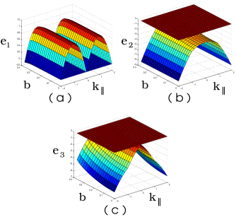
Figure 3: Plot of the real part of the eigenvalues $e_{1}$, $e_{2}$ and $e_{3}$ versus $a$ and $k_{\|}$ for $\lambda=2$. The eigenvalue $e_{1}$ is positive for all values of $a$ and $k_{\|}$ indicating linear instability.

The inhomogeneous helical steady state was suggested by the chiral nature of the driving. It would be a hard task to do an exhaustive check of all inhomogeneous configurations for possible steady states. Our strategy is therefore to solve the noiseless equations of motion (4) numerically starting from generic initial configurations in both $1$ and $2$ dimensions. The dynamics could either take the system to some other non-trivial inhomogeneous stationary state or lead to temporally periodic or chaotic configurations Wolfram (1984).

The numerical scheme for solving Eq. (4) should be chosen carefully as the linear derivative in the drive would give rise to numerical instabilities if the standard Euler scheme of discretization were implemented Press et al. (1992). We adopt an operator splitting method Press et al. (1992) which allows us to treat the dissipative terms and the drive separately under different discretization schemes. The dissipative part is solved using the standard Euler method Seigert and Rao (1993) and for the drive we use the following algorithm. The time evolution of the spins with the drive alone is a precession about the local magnetic field ${\vec{h}}({\bf x},t)=\partial_{\|}{\vec{S}}({\bf x},t)$. If ${\vec{h}}({\bf x},t)$ were a constant in space and time, the local spin ${\vec{S}}({\bf x},t)$ would have precessed about this field, keeping its magnitude $|{\vec{S}}|$ fixed but changing its azimuthal angle $\phi$ (taking the direction of ${\vec{h}}$ as the $z-$axis) by $|{\vec{h}}({\bf x},t)|\triangle t$ in a time interval of $\triangle t$. This would have been exact if the field ${\vec{h}}$ were a constant ; in our case however ${\vec{h}}({\bf x},t)$ depends on space and time and we introduce errors of $O(\triangle t)$. We choose $\triangle t$ small enough so as to reduce this error. The advantage of this method is that it does not give rise to numerical instabilities and automatically preserves the magnitude of the local spin $|{\vec{S}}|$ in time. In the simulation space and time are discretized with $\triangle x=1$ and $\triangle t=0.0001$ on a system of size $N=200$ (large enough to avoid finite size effects) with periodic boundary conditions. The local field is calculated by the rule ${\vec{h}}_{i}=({\vec{S}}_{i+1}-{\vec{S}}_{i-1})/\triangle x$. This field is used to update the local spin by the precession algorithm.

Using this numerical scheme we can compute the time series of observables like the magnetization and energy $E=\int dx(\nabla{\vec{S}})^{2}$. We first note that these quantities never seem to settle to a constant value, strongly suggesting that no stable steady state exists. The motion could therefore be either (quasi)periodic or chaotic. This should be revealed in a power spectrum analysis ; regular periodic motion would appear as a set of sharp delta functions. In Fig. 4a we display the power spectrum $P(\omega)=|M_{3}(\omega)|^{2}$ of the third component of the total magnetization $M_{3}=\langle S_{3}\rangle$ for data collected over more than $3$ decades. The displayed spectrum has a clear smooth component with some small features which may be erased by more averaging and more sophisticated binning. In addition, we find that the power spectrum follows a power law ($1/\omega^{2}$) behavior over roughly 2 decades. The power spectrum of the total energy shows a similar behavior. These results strongly suggest that the dynamics is temporally chaotic Cross and Hohenberg (1993). We have also checked that this chaotic behavior shows up from a variety of initial configurations. The power spectrum we obtain from a study of our model in 2 space dimensions shows similar features (Fig. 4b).

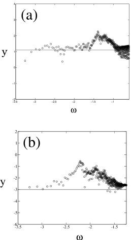
Figure 4: (a) Log-log plot of $y=\sqrt{\omega^{2}|M_{3}(\omega)|^{2}}$ versus $\omega$ in $d=1$ showing the $1/\omega^{2}$ dependence of the power spectrum over approximately $1.5$ decades. (b) Same plot for $d=2$.

Since the components of spin obey partial differential equations (PDEs), we also check for spatial chaos. This is best visualized by constructing space-time plots of local quantities. For instance, Fig. 5a is a space-time plot of the signed local pitch, sgn$(p)\equiv$sgn$(\partial_{x}\phi)$, suggesting spatio-temporal chaosCross and Hohenberg (1993).

We also evaluate, in $d=1$, the space-time correlators of the spin $C(x,t)=\langle{\vec{S}}({\bf x}+{\bf x}^{{}^{\prime}},t+t^{{}^{\prime}})\cdot{\vec{S}}({\bf x}^{{}^{\prime}},t^{{}^{\prime}})\rangle$ in this spatiotemporally chaotic phase. Fig. 5b shows that the equal-time spatial correlation function $C(x,0)$, decays exponentially with a correlation length of the order of the lattice spacing. On the other hand, the unequal-time correlator $C(0,t)$, seems to have a power-law over slightly more than a decade with an exponent $0.7$. While this is not inconsistent with spatio-temporal chaos Cross and Hohenberg (1993), one generally expects power law correlations in non-critical systems only if a conservation law or a Goldstone mode is present. We do not understand the origin of this power law decay at present,

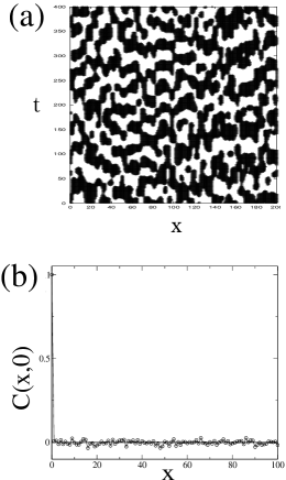
Figure 5: (a) Space-time plot of the signed local pitch, sgn$(p)\equiv$ sgn$(\partial_{x}\phi)$ (black and white patches denote sgn$(p)=\pm 1$ respectively), revealing spatio-temporal chaos. (b)Plot of equal-time correlation function $C(x,0)$ vs $x$ (see text).

Admittedly such characterizations of spatio-temporal chaos are only suggestive and should be made rigorous by studying the dependence of the number of positive Lyapounov exponents on system size. In spite of this, we hope we have provided convincing evidence that the asymptotic configurations in the low drive-temperature regime exhibit spatio-temporal chaos. The numerical evidence we presented was for $d=1$ and $2$, and though we cannot be sure whether this spatio-temporal chaos will persist at higher spatial dimensions, we feel that this is quite likely. This is because in our stability analysis of steady states done for arbitrary spatial dimension, we failed to find any reasonable stable steady state configuration at low drive-temperatures. Moreover, a Lyapunov stability analysis of the simpler equation $\partial_{t}{\vec{S}}=\lambda{\vec{S}}\times\partial_{\|}{\vec{S}}$ in arbitrary $d$ reveals that a tiny disturbance in the initial conditions grows exponentially in time. Several questions arise, to which we do not have answers at present, such as whether there exists a low-dimensional chaotic attractor and if so what is its nature and dimensionality.

The spatio-temporal chaotic phase that we just discovered has embedded in it an infinity of unstable (spatially) periodic steady states. It seems likely Shinbrot et al. (1993); Shinbrot (1995) that starting from generic initial conditions the configuration of spins would eventually visit these periodic steady states, although the time taken to visit any one of these periodic configurations is unpredictable. Since these periodic steady states are unstable, once visited, the dynamics will veer the spin configurations away from it. We now ask whether we can arrange that the spin configuration stays put in a prescribed periodic steady state having visited it ? This is the subject of control of spatiotemporally chaotic systems, one of the most important problems in modern chaos research Shinbrot et al. (1993); Shinbrot (1995). There are two aspects to the control of chaos, stabilisation and targeting. Holding the periodic steady state having visited it is termed stabilization. However since the time taken for this visit from an arbitrary initial condition can be extremely large, it is desirable to target a prescribed unstable periodic steady state. There have been many proposals for controlling chaos in finite dimensional dynamical systems Shinbrot et al. (1993); Shinbrot (1995). However there has been very little work in the more important area of control of spatio-temporal chaos in PDEs (which correspond to an infinite dimensional dynamical system, see Ref. Shinbrot (1995) for a review). Accordingly, it is significant that we are able to stabilize, target, and hence control spatiotemporal chaos in our model, as we now show.

V Targeting and Control: Emergence of Helical states

The helix solutions of Eq. (35) for $v<0$ are an infinite family of unstable spatially periodic steady states of the type discussed in Shinbrot et al. (1993). These helical steady states are parametrized by $a$, the projection of the spin along the $\perp$ axis, $p$, the inverse pitch, and $b$, the projection of the spin along the $\|$ axis. Can chaos in our model be controlled so as to stabilize and target Shinbrot et al. (1993) these helical states? Our control strategy focuses on the spin component $S_{3}$. Thus for instance, in order to stabilize a specific helical configuration (with fixed $a$, $b$ and $p$), we could in principle wait till the dynamics (presumably ergodic) eventually leads to this configuration, after which we apply small perturbations to prevent $S_{3}$ from deviating from the value $b$. This successfully stabilizes the prescribed helix, Fig. 6.

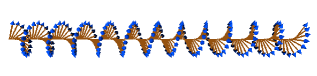
Figure 6: Picture of the stabilized helical configuration from numerical simulations.

In order to target this prescribed helix, we add to (35) terms which would arise from a uniaxial spin anisotropy energy $V_{3}=r_{3}(S_{3}^{2}-b^{2})^{2}$ or $V_{3}=r_{3}(S_{3}-b)^{2}$. We find that a sufficiently large and positive $r_{3}$ forces $S_{3}$ to take the value $b$ exponentially fast starting from arbitrary initial configurations. The subsequent evolution, given by Eq. (35) on setting $S_{3}=b$ is (in $d$ dimensions),

$$\frac{\partial\rho}{\partial t} = \nabla^{2}\rho-\rho(\nabla\phi)^{2}+\rho-(\rho^{2}+b^{2})\rho-\lambda b\rho\partial_{\|}\phi\,,$$

$$\frac{\partial\phi}{\partial t} = \nabla^{2}\phi+\frac{2}{\rho}({\bf\nabla}\rho)\cdot({\bf\nabla}\phi)+\frac{\lambda b}{\rho}(\partial_{\|}\rho)\,.$$ (49)

We now note that these equations can be recast as purely relaxational dynamics,

$$\frac{\partial\rho}{\partial t} = -\frac{\delta F}{\delta\rho}\,,$$

$$\frac{\partial\phi}{\partial t} = -\frac{1}{\rho^{2}}\frac{\delta F}{\delta\phi}\,,$$ (50)

where the ‘free-energy functional’ $F$ has the form of a chiral XY model Chaikin and Lubensky (1998),

$$F = \frac{1}{2}\int d^{d}x\bigg{[}(\nabla\rho)^{2}+\rho^{2}(\nabla\phi)^{2}-(\rho^{2}+b^{2})$$ (51)

$$+\frac{1}{2}(\rho^{2}+b^{2})^{2}+\lambda b\rho^{2}\partial_{\|}\phi\bigg{]}\,.$$

It is easy to see, using the chain-rule, that $F$ is a Lyapunov functional of the dynamics Kampen (1985),

$$\frac{dF}{dt} = \int d^{d}x\left(\frac{\delta F}{\delta S_{1}}\frac{\partial S_{1}}{\partial t}+\frac{\delta F}{\delta S_{2}}\frac{\partial S_{2}}{\partial t}\right)$$ (52)

$$= \int d^{d}x\left[-\bigg{(}\frac{\delta F}{\delta S_{1}}\bigg{)}^{2}-\bigg{(}\frac{\delta F}{\delta S_{2}}\bigg{)}^{2}\right]<0\,,$$

which decreases monotonically in time. Completing the squares, we see that $\partial_{\|}\phi$ appears in $F$ in the combination $(1/2)\rho^{2}(\partial_{\|}\phi+\lambda b/2)^{2}$, which is minimized by the helix $\phi=-(1/2)\lambda bx_{\|}$. Hence starting from any initial configuration the system plummets towards the minimum of this $F$, which is a unique helix with parameters $b$, $a$ and $p$ ($p$ is related to $a$ and $b$ via Eq. (37)). That there is a unique minimum can also be seen by determining the ‘free-energy’ $F_{h}$ of the helical configurations from Eq. (51) and plotting $F_{h}[p,a]$ against $p$ and $a$ (Fig. 7).

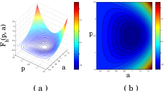
Figure 7: (a) Contour plot of the ‘free-energy’ $F_{h}$ as a function of $a$ and $p$. (b) Projection of plot (a) on the $pa$-plane. It is clear from the plots that there is a unique helical minimum.

The stability of this ‘free-energy’ minimizing helix can also be tested directly from Eq.(49). As before, we perturb about this helix : $\rho=a+{\tilde{\rho}}({\bf x},t)$, and $\phi=px_{\|}+c+{\tilde{\phi}}({\bf x},t)$, and deduce the growth of these perturbations to linear order,

$$\frac{\partial\tilde{\rho}}{\partial t} = \nabla^{2}\tilde{\rho}-2a^{2}\tilde{\rho}-a(2p+\lambda b)\partial_{\|}\tilde{\phi}\,,$$

$$\frac{\partial\tilde{\phi}}{\partial t} = \nabla^{2}\tilde{\phi}+\frac{1}{a}(2p+\lambda b)\partial_{\|}\tilde{\rho}\,.$$ (53)

By going to Fourier space we may evaluate the eigenvalues $\omega_{1}({\bf k})$ and $\omega_{2}({\bf k})$ of the dynamical matrix, given by

$$\omega_{1,2}({\bf k})=-(k^{2}_{\|}+k^{2}_{\perp}+a^{2})\pm\bigg{\{}a^{2}+k^{2}_{\|}(2p+\lambda b)^{2}\bigg{\}}^{1/2}\,.$$ (54)

The helix configuration is stable if these two eigenvalues have negative real parts for all ${\bf k}$, which they do, as can be seen numerically by substituting the values $a$ and $p$ take at the ‘free-energy’ minimum in the above expression.

Let us now see whether our control is robust against noise. Indeed no discussion of the control of spatio-temporal chaos is complete without considering the effects of noise which might result in occasional escapes from the otherwise well controlled system. Do these escapes lead to an instability of the targeted configuration ? We therefore modify (53) by including the nonconservative Gaussian white noises $\eta_{\rho}$ and $\eta_{\phi}$ to linear order. We shall declare the controlled helical state to be robust if the means $\langle\tilde{\rho}\rangle$ and $\langle\tilde{\phi}\rangle$ vanish and the variances are finite in the thermodynamic limit. We therefore ask for the statistics of small fluctuations with Fourier components $\tilde{\rho}_{\bf k}(t)$ and $\tilde{\phi}_{\bf k}(t)$ about the controlled helical state, where $2\pi/L<k<\Lambda$ for a system of linear extent $L$ ($\Lambda$ is the ultraviolet cutoff). It is clear from (53) that the means $\langle\tilde{\rho}_{\bf k}\rangle$ and $\langle\tilde{\phi}_{\bf k}\rangle$ decay exponentially to zero: the relaxation time for $\tilde{\rho}_{\bf k}$ is finite at small $k$, whereas that for $\tilde{\phi}_{\bf k}$ goes as $k^{-2}$.

To calculate the variances, note that the dynamics is governed in the mean by the Lyapounov functional (51), and that the noise is spatiotemporally white. It follows Chaikin and Lubensky (1998) that the steady-state configuration probability $P[\rho,\phi]\propto e^{-cF}$ where $c$ is an effective inverse temperature. Since $F\simeq\int[{\rm const}(\tilde{\rho})^{2}+{\rm const}(\nabla\tilde{\phi})^{2}]$ for small fluctuations about the helical minimum, i.e., $P$ is approximately gaussian, this immediately implies that $\langle|\tilde{\phi}_{\bf k}|^{2}\rangle\sim k^{-2}$ and $\langle|\tilde{\rho}_{\bf k}|^{2}\rangle\sim{\rm const.}$ for small $k$. Thus the variance $\langle\tilde{\rho}^{2}\rangle=\int_{k}\langle|\tilde{\rho}_{\bf k}|^{2}\rangle$ ($2\pi/L<k<\Lambda$), is $L$-independent for $L\to\infty$ in any dimension $d$, whereas $\langle\tilde{\phi}^{2}\rangle=\int_{k}\langle|\tilde{\phi}_{\bf k}|^{2}\rangle$ diverges as $L$ and $\ln L$ respectively for $d=1$ and $2$, and is finite for $d>2$.

To obtain a more explicit asymptotic form for the the variance we calculate the equal-time correlation functions $C_{\tilde{\rho}}({\bf k},t)=\langle\tilde{\rho}_{\bf k}(t)\tilde{\rho}_{-{\bf k}}(t)\rangle$ and $C_{\tilde{\phi}}({\bf k},t)=\langle\tilde{\phi}_{\bf k}(t)\tilde{\phi}_{-{\bf k}}(t)\rangle$ from the linearized equations of motion,

$$\frac{\partial\tilde{\rho}}{\partial t} = \nabla^{2}\tilde{\rho}-2a^{2}\tilde{\rho}-(2ap+\lambda ab)\partial_{\|}\tilde{\phi}+\eta_{\rho}\,,$$

$$\frac{\partial\tilde{\phi}}{\partial t} = \nabla^{2}\tilde{\phi}+\frac{1}{a}(2p+\lambda b)\partial_{\|}\tilde{\rho}+\eta_{\phi}\,,$$ (55)

where $\eta_{\rho}({\bf x},t)=\eta_{1}({\bf x},t)\cos(px_{\|})+\eta_{2}({\bf x},t)\sin(px_{\|})$ and $\eta_{\phi}({\bf x},t)=a^{-1}[\eta_{2}({\bf x},t)\cos(px_{\|})-\eta_{1}({\bf x},t)\sin(px_{\|})]$. The noises $\eta_{\rho}({\bf k},t)$ and $\eta_{\phi}({\bf k},t)$ satisfy

$$\langle\eta_{\rho}({\bf k},t)\eta_{\rho}({\bf k}^{\prime},t^{\prime})\rangle = 2B\delta_{{\bf k},-{\bf k}^{\prime}}\delta(t-t^{\prime})\,,$$

$$\langle\eta_{\phi}({\bf k},t)\eta_{\phi}({\bf k}^{\prime},t^{\prime})\rangle = \frac{2B}{a^{2}}\delta_{{\bf k},-{\bf k}^{\prime}}\delta(t-t^{\prime})\,,$$

$$\langle\eta_{\rho}({\bf k},t)\eta_{\phi}({\bf k}^{\prime},t^{\prime})\rangle = 0\,.$$ (56)

We may easily solve Eq. (55) for Fourier transforms $\rho_{\bf k}$ and $\phi_{\bf k}$,

$$\tilde{\rho}_{\bf k}(\omega) = \frac{1}{D({\bf k},\omega)}(\eta_{\rho}({\bf k},\omega)(i\omega+k^{2})$$

$$-i\eta_{\phi}({\bf k},\omega)k_{\|}a(2p+\lambda b))\,,$$

$$\tilde{\phi}_{\bf k}(\omega) = \frac{1}{D({\bf k},\omega)}(\eta_{\phi}({\bf k},\omega)(i\omega+k^{2}+2a^{2})$$ (57)

$$-\frac{i}{a}\eta_{\rho}({\bf k},\omega)k_{\|}(2p+\lambda b))\,,$$

where

$$D({\bf k},\omega)=-\omega^{2}+2i\omega(k^{2}+a^{2})+k^{2}(k^{2}+2a^{2})-k_{\|}^{2}(2p+\lambda b)^{2}\,.$$ (58)

We now compute the equal time correlation functions $C_{\tilde{\rho}}$ and $C_{\tilde{\phi}}$ averaged over the noise:

$$C_{\tilde{\rho}}({\bf k}) = \langle\tilde{\rho}_{\bf k}(t)\tilde{\rho}_{-{\bf k}}(t)\rangle=\int d^{-}\omega\langle\tilde{\rho}_{\bf k}(\omega)\tilde{\rho}_{-{\bf k}}(-\omega)\rangle$$ (59)

$$= B\frac{k^{4}+k_{\|}^{2}a^{2}(2p+\lambda b)^{2}}{2f_{+}f_{-}(f_{+}+f_{-})}+\frac{B}{2(f_{+}+f_{-})}$$

where $f_{+}$ and $f_{-}$ are the roots of the equation $D({\bf k},\omega)=0$,

$$f_{\pm}=k^{2}+a^{2}\pm\bigg{[}a^{4}+k_{\|}^{2}(2p+\lambda b)^{2}\bigg{]}^{1/2}\,.$$ (60)

and

$$C_{\tilde{\phi}}({\bf k}) = \langle\tilde{\phi}_{\bf k}(t)\tilde{\phi}_{-{\bf k}}(t)\rangle=\int d^{-}\omega\langle\tilde{\phi}_{\bf k}(\omega)\tilde{\phi}_{-{\bf k}}(-\omega)\rangle$$ (61)

$$= \frac{B}{a^{2}}\frac{k^{2}+2a^{2}+k_{\|}^{2}(2p+\lambda b)^{2}}{2f_{+}f_{-}(f_{+}+f_{-})}$$

$$+\frac{B}{2a^{2}}\frac{1}{f_{+}+f_{-}}\,.$$

We use the $k\rightarrow 0$ behavior to evaluate the variances $\Delta_{\tilde{\rho}}$ and $\Delta_{\tilde{\phi}}$. In this infrared limit

$$C_{\tilde{\rho}}({\bf k},t) \sim \frac{B}{k^{2}+a^{2}}\,,$$

$$C_{\tilde{\phi}}({\bf k},t) \sim \frac{B}{k^{2}_{\perp}+k^{2}_{\|}\bigg{(}1-\left(\frac{2p+\lambda b}{a}\right)^{2}\bigg{)}}\,.$$ (62)

The variances $\Delta_{\tilde{\rho}}$ and $\Delta_{\tilde{\phi}}$ obtained on integrating the correlators over all ${\bf k}$ and then taking the thermodynamic limit $L\to\infty$ depend sensitively on the spatial dimension $d$. The variance of $\tilde{\rho}$ is finite in all dimensions,

$$\Delta_{\tilde{\rho}}=\left\{\begin{array}[]{ll}\pi/a&\mbox{$d=1\,\,,$}\\ \ln(1+(\Lambda/a)^{2})&\mbox{$d=2\,\,,$}\\ \mbox{finite}&\mbox{$d=3\,\,,$}\end{array}\right.$$ (63)

while the variance of $\tilde{\phi}$ diverges in $1$ and $2$ dimensions and is finite in higher dimensions,

$$\Delta_{\tilde{\phi}}=\left\{\begin{array}[]{ll}L&\mbox{$d=1\,\,,$}\\ \ln L&\mbox{$d=2\,\,,$}\\ \mbox{finite}&\mbox{$d=3\,\,.$}\end{array}\right.$$ (64)

Thus occasional excursions from the controlled state as a result of the noise do not lead to an instability of the targeted state for $d>2$; the behavior for $d\leq 2$ is no worse than for a thermal equilibrium $XY$ model.

VI Discussions and Future Directions

In this paper we have constructed the simplest example of a spatially extended dynamics in which dissipation, (reversible) precession and spatially anisotropic driving act in concert to produce spatio-temporal chaos in a whole region of parameter space. The model, the classical Heisenberg magnet in $d$ space dimensions, is driven by imposing a background steady current of heat or particles (or any other mobile species) which couples to the Heisenberg spins. Our driven Heisenberg model (DHM) is a natural generalization of the DDLG models to the case of a 3-component axial-vector order parameter ${\vec{S}}$, and is an important step in the exploration of dynamic universality classes Hohenberg and Halperin (1977) far from equilibrium Täuber et al. (2002); Marculescu and Ruiz (1998).

In the limit where the mobile species is ‘fast’, the imposed steady current alters the effective dynamics of the isotropic magnet so as to generate a driven precession term $\lambda{\vec{S}}\times\partial_{\|}{\vec{S}}$, that is responsible for all the remarkable phenomena we predict. We summarize the nature of the asymptotic configurations in a ‘non-equilibrium phase diagram’, Fig. 8, as a function of the drive-temperature $v$. The system exhibits a ‘paramagnetic steady state’ at high $v$ and a ‘critical steady state’ at $v=0$, with power-law correlations induced by the driving even when the equilibrium Heisenberg magnet (without the driving) is paramagnetic. The drive takes the system away from the Wilson-Fisher fixed point leading to a new drive induced universality class. At low drive-temperatures both the homogeneous and inhomogeneous steady states are unstable. In particular, the system has an infinity of spatially periodic unstable steady states which are helical. We have provided evidence, at least in $d=1$ and $2$, that the dynamics at low $v$ is spatio-temporally chaotic. We have found that the spatio-temporal chaos may be ‘controlled’ to target any desired helical steady state. This control works even in the presence of noise in dimensions $d>2$. The generic occurence of spatio-temporal chaos in our model is encouraging, given the intriguing formal similarity to the nonlinearity $({\bf v}\cdot{\nabla}){\bf v}$ in the Navier Stokes equation.

Our criterion for declaring the low temperature phase as spatio-temporally chaotic is based on rather well established tests of power-spectrum analysis, space-time plots and decay of space-time correlators. Admittedly such characterization is not very rigorous; ideally one would like to analize the system size $L$ dependence of the Lyapounov spectrum. We leave this for future investigation, as also several questions regarding this spatio-temporal chaotic regime, such as the existence and nature of a low dimensional attractor or the possibility of complex ordered states in higher dimensions,

Note that while the entire low drive-temperature phase is chaotic, the critical phase is not; the DRG analysis definitely shows a stable fixed point in all dimensions. This is quite different from the possibility of a chaotic critical point, discussed in Ref. Täuber et al. (2002), for a general class of anisotropically driven $O(n)$ models along $d_{\parallel}$ directions. Their driving appears as a nonequilibrium source of noise which is not bound by a fluctuation-dissipation relation. At the critical point of this model they find, to 1-loop, no stable fixed point when $d_{\parallel}>d_{\parallel}^{*}$. They tentatively put forward the possibility of spatio-temporal chaos at criticality. There have been earlier suggestions of chaotic criticality in equilibrium critical behavior, albeit in systems with quenched disorder Boyanovski and Cardy (1982).

We conclude this paper by reminding the reader again of the variety of explicit lattice and continuum realizations of our driven dynamics discussed in Sect.IIB . We hope that this will stimulate a search for experimental systems, e.g., isotropic magnets carrying a steady particle or heat current, as well as model magnetized lattice-gas simulations, where the predictions of our model can be tested.

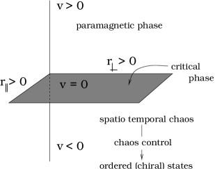
Figure 8: Non-equilibrium phase diagram as a function of the drive-temperature $v$.

Appendix A

In this Appendix we present the details of perturbative calculation mentioned in Sect. IV. The diagrams corresponding to the lowest order terms in the perturbation expansion are constructed following the rules shown in Fig. 9.

Corrections to $G_{0}({\bf k},\omega)$

(I) Corrections from the $\lambda$ vertex :

Graphs (I) and (II) in Fig. 10 show the one-loop corrections to $G_{0}({\bf k},\omega)$ due to the $\lambda$ vertex.

$$\Sigma_{\lambda}({\bf k},\omega)=-\frac{\lambda^{2}}{4}\int d^{-}qd^{-}\nu\bigg{[}(q_{\|}-(k_{\|}-q_{\|}))(k_{\|}-(-q_{\|}))G_{0}({\bf k}-{\bf q},\omega-\nu)C_{0}({\bf q},\nu)$$

$$+((k_{\|}-q_{\|})-q_{\|})(k_{\|}+(k_{\|}-q_{\|}))G_{0}({\bf q},\nu)C_{0}({\bf k}-{\bf q},\omega-\nu)\bigg{]}$$

$$=-\frac{2\lambda^{2}B}{4}\int d^{-}q\bigg{[}\frac{(2q_{\|}-k_{\|})(k_{\|}+q_{\|})}{\gamma^{2}({\bf q})}+\frac{(k_{\|}-2q_{\|})(2q_{\|}-q_{\|})}{\gamma^{2}({\bf k}-{\bf q})}\bigg{]}\frac{1}{\gamma^{2}({\bf q})+\gamma^{2}({\bf k}-{\bf q})}\,.$$ (65)

In the above integrals $\gamma^{n}({\bf k})$ is defined as

$$\gamma^{n}({\bf k})=\bigg{(}r_{\|}k_{\|}^{2}+r_{\perp}k_{\perp}^{2}+v\bigg{)}^{n}.$$

We expand $\Sigma_{\lambda}({\bf k},0)$ in powers of $k_{\|}$ and $k_{\perp}$. Terms which are higher order than $O(k_{\|}^{2})$ or $O(k_{\perp}^{2})$ are ultraviolet convergent. Coefficients of the terms of order ${k}^{0}$, $k_{\|}^{2}$ and $k_{\perp}^{2}$ denote changes to $v$, $r_{\|}$ and $r_{\perp}$ respectively.

Figure 9: Graphs for correlation functions and vertices at the tree level. $F_{\alpha\beta\gamma\delta}=(1/3)[\delta_{\alpha\beta}\delta_{\gamma\delta}+\delta_{\alpha\delta}\delta_{\beta\gamma}+\delta_{\alpha\gamma}\delta_{\beta\delta}]$.

(i) Term proportional to ${k}^{0}$

This part of $\Sigma_{\lambda}({\bf k},0)$ does not have any infrared divergences but has divergences in the ultraviolet. We introduce an upper momentum cutoff $\Lambda$ to get an estimate of the correction to $v$. We will denote the self energy contribution coming from the $\lambda$ vertex to order $k^{0}$ as $(\Sigma_{0})_{\lambda}$,

$$(\Sigma_{0})_{\lambda} =-\frac{\lambda^{2}B}{2}\int d^{-}q\frac{q_{\|}^{2}}{\gamma^{4}({\bf q})}$$ (66)

$$=-\frac{\pi\Lambda\lambda^{2}B}{4r_{\|}^{3/2}r_{\perp}^{1/2}}\,.$$

(ii) Term proportional to $k_{\|}^{2}$

$$(\Sigma_{\|})_{\lambda}= -\frac{\lambda^{2}Bk_{\|}^{2}}{4}\int d^{-}q\bigg{[}\frac{1}{2\gamma^{4}({\bf q})}+\frac{16r_{\|}^{2}q_{\|}^{4}}{\gamma^{8}({\bf q})}-\frac{4r_{\|}q_{\|}^{2}}{\gamma^{6}({\bf q})}\bigg{]}$$ (67)

$$=\frac{\lambda^{2}Bv^{\epsilon/2}r_{\|}k_{\|}^{2}}{8\pi^{2}\epsilon(r_{\|}r_{\perp})^{3/2}}\,,$$

where

$$\int d^{-}q\frac{1}{\gamma^{4}({\bf q})}=\frac{r_{\|}v^{-\epsilon/2}}{8\pi^{2}(r_{\|}r_{\perp})^{3/2}}\frac{1}{\epsilon}\,,$$ (68)

$$\int d^{-}q\frac{q_{\|}^{2}}{\gamma^{6}({\bf q})}=\frac{v^{-\epsilon/2}}{32\pi^{2}(r_{\|}r_{\perp})^{3/2}}\frac{1}{\epsilon}\,,$$ (69)

$$\int d^{-}q\frac{q_{\|}^{4}}{\gamma^{8}({\bf q})}=\frac{r_{\|}v^{-\epsilon/2}}{64\pi^{2}(r_{\|}^{5/2}r_{\perp}^{3/2})}\frac{1}{\epsilon}\,,$$ (70)

have been evaluated using the standard integrals for the general form $\int d^{-}q(q_{\|}^{a}q_{\perp}^{b})/\gamma^{c}({\bf q})$ given in Ref. ’t Hooft and Veltman (1972). We have also had to make use of the asymptotic expansion for the Gamma function $\Gamma(-n+\epsilon)$, when $n$ is zero or any positive integer and $\epsilon\rightarrow 0$,

$$\Gamma(-n+\epsilon)=\frac{(-1)^{n}}{n!}\bigg{[}\frac{1}{\epsilon}+\bigg{(}1+\frac{1}{2}+\ldots+\frac{1}{n}-\gamma\bigg{)}+O(\epsilon)\bigg{]}\,,$$ (71)

where $\gamma$ is the Euler-Mascheroni constant Abramowitz and Stegun (1968).

Figure 10: $O(\lambda^{2})$ corrections to $G_{0}({\bf k},\omega)$.

(iii) Term proportional to $k_{\perp}^{2}$

$$(\Sigma_{\perp})_{\lambda}= -\frac{\lambda^{2}Bk_{\perp}^{2}}{4}\int d^{-}qq_{\|}^{2}\bigg{[}\frac{16r_{\perp}q_{\perp}}{\gamma^{8}({\bf q})}-\frac{4r_{\perp}}{\gamma^{6}({\bf q})}\bigg{]}$$ (72)

$$=-\frac{5\lambda^{2}Br_{\perp}k_{\perp}^{2}v^{-\epsilon/2}}{96\pi^{2}r_{\perp}(r_{\|}r_{\perp})^{3/2}}\frac{1}{\epsilon}\,,$$

where we have evaluated the integral

$$\int d^{-}q\frac{q_{\|}^{2}q_{\perp}^{2}}{\gamma^{8}({\bf q})}=\frac{v^{-\epsilon/2}}{48\pi^{2}r_{\perp}(r_{\|}r_{\perp})^{3/2}}\frac{1}{\epsilon}\,.$$ (73)

(II) Corrections from the $u-$ vertex :
There is also a correction to the propagator $G({\bf k},\omega)$ coming from the $u-$ vertex ; to $O(\epsilon)$ this is shown in the figure below.

Figure 11: $O(u^{2})$ corrections to the ${\bf k}=0$ part of $G_{0}({\bf k},\omega)$.

To 1-loop, the correction to $G({\bf k},\omega)$ from this interaction comes only from the ${\bf k}=0$ piece given by,

$$(\Sigma_{0})_{u} =-\frac{5u}{3}\int d^{-}qd^{-}\nu C_{0}({\bf q},\nu)$$ (74)

$$=-\frac{5uB}{3}\int d^{-}q\frac{1}{\gamma^{2}({\bf q})}$$

$$=-\frac{5\pi\Lambda uB}{6r_{\|}^{1/2}r_{\perp}^{3/2}}\,.$$

The net 1-loop correction to the propagator $G$ adds up to

$$\Sigma({\bf k},\omega)=[(\Sigma_{0})_{\lambda}+(\Sigma_{0})_{u}]+(\Sigma_{\|})_{\lambda}k_{\|}^{2}+(\Sigma_{\perp})_{\lambda}k_{\perp}^{2}\,.$$ (75)

Corrections to $C_{0}({\bf k},\omega)$

Figure 12: $O(\lambda^{2})$ corrections to $C_{0}({\bf k},\omega)$.

$$\Sigma_{B}= -\frac{\lambda^{2}}{4}\int d^{-}qd^{-}\nu((k_{\|}-q_{\|})-q_{\|})(q_{\|}-(k_{\|}-q_{\|}))C_{0}({\bf k}-{\bf q},\omega-\nu)C_{0}({\bf q},\nu)$$ (76)

$$=\lambda^{2}B^{2}\int d^{-}q\frac{q_{\|}^{2}}{\gamma^{6}({\bf q})}$$

$$=\frac{\lambda^{2}B^{2}v^{-\epsilon/2}}{32\pi^{2}(r_{\|}r_{\perp})^{3/2}}\frac{1}{\epsilon}\,.$$

The renormalized couplings are obtained from the vertex corrections to $\lambda$ and $u$.

Corrections to the $\lambda-$ vertex
The corrections to $\lambda$ come from the three-point correlators,

Figure 13: $O(\lambda^{3})$ correction to the $\lambda-$ vertex.

The contribution from (I) to the vertex function $\Gamma_{\lambda}$ is given by,

$$\bigg{(}\frac{-i\lambda}{2}\bigg{)}^{3}\int d^{-}qd^{-}\nu\bigg{[}((k_{1\|}-q_{\|})+k_{1\|})((k_{2\|}+q_{\|})+q_{\|})((k_{1\|}+k_{2\|})+(k_{1\|}-q_{\|}))\bigg{]}\times$$

$$G_{0}({\bf q},\nu)G_{0}({\bf k}_{2}+{\bf q},\omega_{2}-\nu)C_{0}({\bf k}_{1}-{\bf q},\omega_{1}-\nu)$$

$$=\frac{i\lambda^{3}B}{16}\int d^{-}q\frac{(8k_{1\|}+k_{2\|})q_{\|}^{2}}{\gamma^{6}({\bf q})}\,.$$ (77)

Likewise the contribution from (II) to $\Gamma_{\lambda}$ is

$$\bigg{(}\frac{-i\lambda}{2}\bigg{)}^{3}\int d^{-}qd^{-}\nu\bigg{[}(-k_{1\|}-q_{\|})((k_{2\|}+q_{\|})+q_{\|})((k_{1\|}+k_{2\|})+(k_{1\|}-q_{\|}))\bigg{]}\times$$

$$G_{0}({\bf k}_{1}-{\bf q},\omega_{1}-\nu)G_{0}({\bf k}_{2}+{\bf q},\omega_{2}-\nu)C_{0}({\bf q},\nu)$$

$$=-\frac{i\lambda^{3}B}{32}\int d^{-}q\frac{(2k_{1\|}+k_{2\|})q_{\|}^{2}}{\gamma^{6}({\bf q})}\,,$$ (78)

while (III) gives

$$\bigg{(}\frac{-i\lambda}{2}\bigg{)}^{3}\int d^{-}qd^{-}\nu\bigg{[}(-(k_{2\|}+q_{\|})-(k_{1\|}+k_{2\|}))((k_{2\|}+q_{\|})+q_{\|})((k_{1\|}-q_{\|})+k_{1\|})\bigg{]}\times$$

$$G_{0}({\bf q},\nu)G_{0}({\bf k}_{1}-{\bf q},\omega_{1}+\nu)C_{0}({\bf k}_{2}+{\bf q},\omega_{1}+\nu)$$

$$=-\frac{i\lambda^{3}B}{32}\int d^{-}q\frac{(2k_{1\|}-5k_{2\|})q_{\|}^{2}}{\gamma^{6}({\bf q})}\,.$$ (79)

The three contributions combine to give

$$\Gamma_{\lambda}(2k_{1\|}+k_{2\|})= \frac{3i\lambda^{3}B}{16}\int d^{-}q\frac{q_{\|}^{2}(2k_{1\|}+k_{2\|})}{\gamma^{6}({\bf q})}$$ (80)

$$=\frac{3i\lambda^{3}B(2k_{1\|}+k_{2\|})v^{-\epsilon/2}}{512\pi^{2}(r_{\|}r_{\perp})^{3/2}}\frac{1}{\epsilon}\,.$$

Corrections to the $u-$ vertex
There are two contributions to the vertex function $\Gamma_{u}$ to $O(u^{2})$ and $O(\lambda^{4})$.

Figure 14: $O(u^{2})$ correction to the $u-$ vertex.

The $O(u^{2})$ graph gives

$$F_{\alpha\beta\gamma\delta}\frac{11u^{2}}{9}\int d^{-}qd^{-}\nu C_{0}({\bf q},\nu)G_{0}({\bf k}_{1}+{\bf k}_{2}-{\bf q},\omega_{1}+\omega_{2}-\nu)$$

$$= F_{\alpha\beta\gamma\delta}\frac{11u^{2}B}{18}\int d^{-}q\frac{1}{\gamma^{4}({\bf q})}$$

$$= F_{\alpha\beta\gamma\delta}\frac{11u^{2}B}{48\pi^{2}r_{\perp}^{3/2}r_{\|}^{1/2}}\frac{1}{\epsilon}\,.$$ (81)

Figure 15: $O(\lambda^{4})$ correction to the $u-$ vertex.

The $O(\lambda^{4})$ graph gives the following contribution :

$$-1152F_{\alpha\beta\gamma\delta}\bigg{(}\frac{\lambda}{4}\bigg{)}^{4}\int d^{-}qd^{-}\nu((k_{1\|}-q_{\|})-q_{\|})(k_{4\|}-(k_{1\|}-k_{4\|}-q_{\|}))(k_{3\|}-(k_{2\|}+q_{\|}))(k_{2\|}+q_{\|})\times$$

$$G_{0}({\bf k}_{1}-{\bf q},\omega-\nu)G_{0}({\bf k}_{1}-{\bf k}_{4}-{\bf q},\omega_{1}-\omega_{2}-\nu)G_{0}({\bf k}_{2}+{\bf q},\omega_{2}+\nu)C_{0}({\bf q},\nu)$$

$$-1152F_{\alpha\beta\gamma\delta}\bigg{(}\frac{3\lambda^{4}B}{4^{3}}\bigg{)}\int d^{-}q\frac{q_{\|}^{2}}{\gamma^{8}({\bf q})}$$

$$=-F_{\alpha\beta\gamma\delta}\frac{27\lambda^{4}}{32\pi^{2}r_{\perp}^{3/2}r_{\|}^{1/2}\epsilon}\,.$$ (82)

The net correction to the $u-$ vertex is,

$$\Gamma_{u} =F_{\alpha\beta\gamma\delta}\frac{11u^{2}B}{48\pi^{2}r_{\perp}^{3/2}r_{\|}^{1/2}}\frac{1}{\epsilon}-F_{\alpha\beta\gamma\delta}\frac{27\lambda^{4}}{32\pi^{2}r_{\perp}^{3/2}r_{\|}^{1/2}\epsilon}$$ (83)

$$=F_{\alpha\beta\gamma\delta}(r_{\|}^{1/2}r_{\perp}^{3/2})\bigg{[}\frac{11\pi^{4}\kappa^{2}}{12B\epsilon}-\frac{27\pi^{4}\tau^{2}}{8B\epsilon}\bigg{]}\,,$$

where $\kappa$ and $\tau$ are defined by

$$\kappa=\frac{uB}{2\pi^{3}(r_{\|}^{1/2}r_{\perp}^{3/2})}\,,$$ (84)

$$\tau=\frac{\lambda B}{2\pi^{3}(r_{\|}^{3/2}r_{\perp}^{3/2})}\,.$$ (85)

References

- Das et al. (2002) J. Das, M. Rao, and S. Ramaswamy, Europhys. Lett. 60 (2002).
- Täuber et al. (2002) U. C. Täuber, V. K. Akkineni, and J. E. Santos, Phys. Rev. Lett. 88, 045702 (2002).
- Täuber et al. (1999) U. Täuber, J. Santos, and Z. Racz, Eur. Phys. J. B 7, 309 (1999).
- Antal et al. (1999) T. Antal, A. R. Z. Raćz, and G. M. Schütz, Phys. Rev. E 59, 4912 (1999).
- Eisler et al. (2003) V. Eisler, Z. Raćz, and F. van Wijland, Phys. Rev. E 67, 056129 (2003).
- Schmittmann and Zia (1995) B. Schmittmann and R. K. P. Zia, Phase Transitionsand Critical Phenomena, vol. 17 (Academic Press, NY, 1995).
- Marro and Dickman (1999) J. Marro and R. Dickman, Nonequilibrium Phase Transitions in Lattice Models (Cambridge University Press, Cambridge, 1999).
- Ma and Mazenko (1975) S.-K. Ma and G. Mazenko, Phys. Rev. B 11, 4077 (1975).
- Fogedby (13) H. C. Fogedby, J. Phys. A 1980, 1476 (13).
- Hohenberg and Halperin (1977) P. Hohenberg and B. Halperin, Rev. Mod. Phys. 49, 435 (1977).
- Marculescu and Ruiz (1998) S. Marculescu and F. R. Ruiz, J. Phys. A 31, 8355 (1998).
- Forster et al. (16) D. Forster, D. R. Nelson, and M. J. Stephen, Phys. Rev. A 732, 1977 (16).
- Balakrishnan (1982) R. Balakrishnan, J. Phys. C 15, L1305 (1982).
- Kardar et al. (1986) M. Kardar, G. Parisi, and Y. C. Zhang, Phys. Rev. Lett. 56, 889 (1986).
- (15) Thus, despite the superficial resemblance of this nonlinearity to that in the stochastic Burgers equation Schmittmann and Zia (1995), there is no “height” representation [M. Kardar, G. Parisi, and Y. C. Zhang, Phys. Rev. Lett. 56, 889 (1986)] for Eqn. (4).
- Belavin and Polyakov (1975) A. A. Belavin and A. M. Polyakov, JETP Lett. 22, 245 (1975).
- Rajaraman (1982) R. Rajaraman, Instantons and Solitons (North Holland, Amsterdam, 1982).
- Lau et al. (2003) A. W. C. Lau, B. D. Hoffman, A. Davies, J. C. Crocker, and T. C. Lubensky, Phys. Rev. Lett. 91, 198101 (2003).
- Purcell (1977) E. M. Purcell, Am. J. Phys. 45, 3 (1977).
- Chaikin and Lubensky (1998) P. M. Chaikin and T. C. Lubensky, Principles of condensed matter physics (Cambridge University Press, Cambridge, 1998).
- Kampen (1985) N. G. V. Kampen, Stochastic Processes in Physics and Chemistry (North Holland Physics Publishing, Amsterdam, 1985).
- Medina et al. (1989) E. Medina, T. Hwa, and M. Kardar, Phys. Rev. A 39, 3053 (1989).
- Amit (1978) D. J. Amit, Field Theory, the Renormalisation Group, and Critical Phenomena (Academic Press, NY, 1978).
- Brezin et al. (1976) E. Brezin, J. C. L. Guillon, and Zinn-Justin, Phase Transitions and Critical Phenomena, vol. 6 (Academic Press, NY, 1976).
- ’t Hooft and Veltman (1972) G. ’t Hooft and M. Veltman, Nuc. Phys. B 44, 189 (1972).
- Hwa and Kardar (1992) T. Hwa and M. Kardar, Phys. Rev. A 45, 7002 (1992).
- Wolfram (1984) S. Wolfram, Rev. Mod. Phys. 55, 601 (1984).
- Press et al. (1992) W. H. Press, S. A. Teukolsky, W. T. Vetterling, and B. P. Flannery, Numerical Recipes in Fortran (Cambridge University Press, Cambridge, 1992).
- Seigert and Rao (1993) M. Seigert and M. Rao, Phys. Rev. Lett. 63, 1956 (1993).
- Cross and Hohenberg (1993) M. C. Cross and P. C. Hohenberg, Rev. Mod. Phys. 65, 851 (1993).
- Shinbrot et al. (1993) T. Shinbrot, C. Grebogi, E. Ott, and J. A. Yorke, Nature 363, 411 (1993).
- Shinbrot (1995) T. Shinbrot, Adv. Phys. 44, 73 (1995).
- Boyanovski and Cardy (1982) D. Boyanovski and J. L. Cardy, Phys. Rev. B 26, 154 (1982).
- Abramowitz and Stegun (1968) M. Abramowitz and I. A. Stegun, Handbook of Mathematical Functions (Dover Publications, Inc., NY, 1968), 5th ed.