Phase dependence of localization in the driven two-level model

Abstract

A two-level system subjected to a high-frequency driving field can exhibit an effect termed “coherent destruction of tunneling”, in which the tunneling of the system is suppressed at certain values of the frequency and strength of the field. This suppression becomes less effective as the frequency of the driving field is reduced, and we show here how the detailed form of its fall-off depends on the phase of the driving, which for certain values can produce small local maxima (or revivals) in the overall decay. By considering a squarewave driving field, which has the advantage of being analytically tractable, we show how this surprising behavior can be interpreted geometrically in terms of orbits on the Bloch sphere. These results are of general applicability to more commonly used fields, such as sinusoidal driving, which display a similar phenomenology.

Since the pioneering work of Hänggi and co-workers hanggi_prl it has been known that a quantum system subjected to a periodic driving field can exhibit an unusual effect termed “coherent destruction of tunneling” (CDT), in which the tunneling dynamics of the system are quenched at various specific values of the strength and frequency holthaus of the applied field. One of the simplest systems in which this effect appears is the driven two-level system hanggi_epl , which has been applied to describe many physical situations, such as an electron moving in a double-well potential hanggi_prl , molecular switches lehmann , the single-Cooper-pair box nakamura and superconducting tunnel junctions vion . Controlling the dynamics of such systems has become of increasing importance due to possible technological applications in quantum computing, and the CDT effect provides one method of achieving such control which preserves the quantum coherence of the system.

The periodicity of the driving field allows us to invoke the Floquet theorem, and expand solutions of the time-dependent Schrödinger equation review as

$$\psi(t)=\sum_{j=1}^{2}\ c_{j}\exp[-i\epsilon_{j}t]\phi_{j}(t),$$ (1)

where $\epsilon_{j}$ is termed the quasienergy, and $\phi_{j}(t)$ is a function with the same periodicity as the driving field, called a Floquet state. A necessary condition for CDT to occur is that the quasienergies must be either degenerate or close to degeneracy lehmann . If we neglect the time-dependence of the Floquet states it is clear that the dynamics of the system will indeed be frozen when this condition is satisfied. Neglecting the intrinsic time-dependence of the Floquet states is a reasonable approximation when the frequency of the driving field is high (the “high-frequency limit” hanggi_epl ), as the period of the field is then much shorter than the typical timescale for tunneling processes, given by the Rabi period. At lower frequencies, however, the Floquet states can have a non-trivial time-dependence, and the degree of CDT can be markedly reduced if the Floquet states themselves have a large amplitude of oscillation caveat . In this work we will show that fall-off in CDT produced by this effect has a surprising dependence on the phase of the driving field. Although phase-effects have been briefly noted in previous work bavli , we provide here the first systematic study and explanation of this effect. We shall show how the phase can be chosen to maximize the degree of CDT, and also how certain choices of phase can produce a non-monotonic decay of CDT, containing small local maxima or “revivals”, as was seen previously in Ref.cabron .

We consider a two-level system described by the Hamiltonian

$$H=\frac{\Delta}{2}\ \sigma_{x}+\frac{E}{2}f(t)\ \sigma_{z},$$ (2)

where $\sigma_{i}$ are the standard Pauli matrices. We parameterize the driving field as $Ef(t)$, where $E$ is the strength of the driving, and $f(t)$ is a $T$-periodic function of unit amplitude and frequency $\omega$, which describes the waveform of the driving field. The eigenstates of the undriven system consist of two extended states: namely a symmetric ground state separated by the level splitting, $\Delta$, from the anti-symmetric excited state. To investigate the tunneling dynamics of the system it will prove useful to also define localized states formed by the sum and difference of these eigenstates, which we label as $|L\rangle$ and $|R\rangle$. The degree of tunneling can be conveniently assessed by initializing the system in state $|L\rangle$ and then evolving it in time under the influence of the Hamiltonian (2). By measuring the probability that the system remains in state $|L\rangle$, $P_{L}(t)=\left|\langle\psi(t)|L\rangle\right|^{2}$, we can quantify the degree to which tunneling is suppressed by finding the minimum value of $P_{L}(t)$ attained, which we term the “localization”. When the tunneling is completely destroyed $P_{L}(t)$ does not change with time, and thus the localization is equal to one. Conversely, if the tunneling is not completely suppressed, the localization will take a lower value, and will be zero if the particle is able to completely tunnel from $|L\rangle$ to $|R\rangle$.

We show in Fig.1 the localization produced as the frequency of the driving field is reduced, obtained by the numerical evolution of the system using a Runge-Kutta technique creff , for two types of driving field: a sine wave and a squarewave. For both fields the driving strength was chosen so that the quasienergies of the system were degenerate and so CDT occurs. As was shown in Ref.creff , this degeneracy condition defines a set of smooth one-dimensional curves in $(E,\omega)$ space called “crossing-manifolds” hanggi_epl . When the quasienergies are degenerate it is clear from Eq.(1) that the time-dependence of the system is given solely by the Floquet states. Since these states are periodic, it is sufficient to evolve the system over just one period of the driving to study its properties, giving a considerable saving of computational effort.

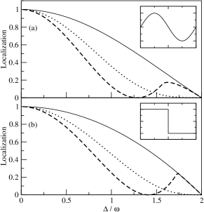
Figure 1: Localization produced by (a) a sinusoidal driving field and (b) a squarewave driving field. Solid line indicates the result for a driving with zero phase-shift, the dotted line for a phase-shift of $\pi/4$, and the dashed line for a phase-shift of $\pi/2$. For high-values of $\omega$ the localization is excellent in all cases, but drops rapidly for $\Delta/\omega>0.5$. For the phase-shift of $\pi/2$ the localization goes through a small local minimum before reaching zero. Insets: A single period of the zero phase-shifted driving fields $f(t)$.

Although the two driving fields are very different, they produce strikingly similar forms of localization. In both cases in the high-frequency regime ($\Delta/\omega\ll 1$) the localization has a value of one, irrespective of the phase of the driving field. This indicates that the tunneling is completely destroyed and thus the system remains frozen in its initial state. As the value of $\omega$ is reduced, the particle is able to tunnel more freely, and the degree of localization falls. It can also be clearly seen that at low frequencies the phase of the driving field has a significant effect on the form of this fall-off. When the field has no phase-shift (shown in the insets to Fig.1) the localization decays monotonically to zero as the frequency is reduced. The initial effect of increasing the phase of the driving field from zero is to cause the localization to drop more rapidly. For example, at $\Delta/\omega=1$ the localization produced by a $\pi/4$ phase-shifted field is half that of the zero phase-shift case, while for a phase shift of $\pi/2$ the localization is about four times smaller. A further effect occurs for values of the phase shift close to its maximum value of $\pi/2$, in which after rapidly decaying to zero,the localization subsequently passes through a small local maximum, before again vanishing at the same frequency as the zero phase-shift case.

To understand how this behavior comes about, it is useful to visualize the dynamics of the two-level system geometrically, by making use of the Bloch sphere representation well-known from quantum optics and NMR studies, and now commonly used in quantum information theory schirmer . Any pure state of the system can be represented by a point on the surface of the Bloch sphere, and we can note in particular that the localized states $|L\rangle$ and $|R\rangle$ correspond to the points $[0,0,\pm 1]$. We shall consider just the case of squarewave driving, as it displays the same phase-dependent behavior as sinusoidal driving, but also has the useful property of allowing exact solutions for the time-development of the system to be obtained. For this form of driving, the time-dependent Hamiltonian (2) decomposes into piecewise constant parts, $H_{\pm}=(\Delta/2)\sigma_{x}\pm(E/2)\sigma_{z}$. These operators can be interpreted conveniently as an interaction between the Bloch vector ${\bf s}$ and a fictitious magnetic field directed along the axes $r_{\pm}=[\Delta,0,\pm E]$, and thus the time-evolution of the system can be viewed as successive Larmor rotations about these axes. This insight is the key to a simple method for interpreting and understanding the dynamics of the system.

The operators $H_{\pm}$ can be exponentiated straightforwardly, yielding the following result for the unitary operator describing the evolution of the system under the influence of $H_{\pm}$:

$$U_{\pm}(t)=I\cos\Omega t-i\frac{\sin\Omega t}{2\Omega}\left[\Delta\ \sigma_{x}\pm E\ \sigma_{z}\right].$$ (3)

In this expression $\Omega=\sqrt{E^{2}+\Delta^{2}}/2$ is the Rabi frequency. The general time-evolution operator for a squarewave driving field can now be expressed simply as the product of successive factors of $U_{\pm}$. Examination of Eq.3 reveals that the propagator for one period of the driving, $U(T)=U_{+}(T/2)U_{-}(T/2)$, is equal to the identity (and thus the quasienergies are both zero and CDT occurs) if $\sin\Omega T/2=0$. This indicates that CDT only arises if the driving frequency is in resonance with the Rabi frequency, $\Omega=n\omega$ where $n$ is an integer. This resonance condition may be expressed alternatively as

$$\left(\frac{E}{\omega}\right)^{2}+\left(\frac{\Delta}{\omega}\right)^{2}=\left(2n\right)^{2}.$$ (4)

It is interesting to note that this equation for the crossing-manifolds for a squarewave driving field, which describes concentric circles in $(E/\omega,\Delta/\omega)$ space, is identical to that hypothesized from purely numerical evidence in Ref.creff .

We now consider the explicit time evolution of the system, and begin with the simplest case of zero phase-shift. The state $|L\rangle$ in which the system is initialized corresponds to the north-pole of the Bloch sphere (${\bf s}=[0,0,1]$). During the first half-period of the driving, this initial state evolves under the influence of $H_{+}$, making a Larmor rotation about the axis $r_{+}$. The resonance condition between the driving frequency $\omega$ and the Larmor frequency means that during this interval the Bloch vector makes $n$ complete revolutions, and thus at $t=T/2$ the system returns to its initial state. During the second half-period a similar process occurs, with the Bloch vector making $n$ revolutions about the axis $r_{-}$. The system thus traces out a symmetric “figure-of-eight” on the surface of the Bloch sphere, as shown in Fig.2. In the high-frequency limit, when $\omega\gg\Delta$ and thus $E\sim\omega$ from Eq.4, the rotation axes are almost parallel to the $z$-axis, and so the loops traced by the Bloch vector have a very small radius. As a result, the orbit remains close to $|L\rangle$ at all times, and the system exhibits a high degree of localization. As $E$ is reduced, however, the angle between the rotation axes increases and the loops traced by the Bloch vector become larger. The system can thus explore further around the Bloch sphere and approach closer to $|R\rangle$, thereby reducing the localization. It is a simple matter to explicitly derive an expression for $P_{L}(t)$, from which the following result for the localization can be obtained

$$P_{L}^{\mbox{min}}=P_{L}(T/4)=1-\frac{\left(\Delta/\omega\right)^{2}}{4n^{2}}.$$ (5)

In Fig.3 it can be seen that this result indeed correctly describes the fall-off in localization for a zero phase-shifted field.

Figure 2: Orbits on the Bloch sphere for driving parameters $\Delta/\omega=1/2$, $E/\omega=\sqrt{15}/2$, i.e. on the first crossing-manifold ($n=1$). The left plot shows the time-evolution for zero phase-shift, and on the right for a phase-shift of $\pi/2$.

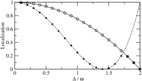
Figure 3: Comparison of the localization on the first crossing-manifold ($n=1$) with the analytical expressions derived in the text. Eq.5 is denoted by the solid line, Eq.6 by the dashed line. It can be seen that for zero-phase shifted driving (hollow circles) the localization is described by Eq.5. For $\pi/2$ phase-shifted driving (solid circles) the localization is given by min $[P_{L}(T/4),P_{L}(T/2)]$, and the crossover between these quantities at $\Delta/\omega=\sqrt{3}$ produces the cusp-like revival feature.

We now consider the effect of the phase-shift. For a phase-shift of $\pi/2$ the system first evolves under $H_{+}$ for a quarter-period, then under $H_{-}$ for an interval of $T/2$, and completes the final quarter-period under $H_{+}$. Accordingly, during the first quarter-period of the driving the Bloch vector makes $n/2$ revolutions about $r_{+}$, and it is thus now important to distinguish whether $n$ is even or odd. In the former case, the Bloch vector will make an integer number of revolutions about $r_{+}$ in the first quarter-period, and so it will end this interval at $|L\rangle$. It will then make $n$ complete revolutions about $r_{-}$ during the next half-period, and will finally complete its motion by making $n/2$ revolutions about $r_{+}$. For even values of $n$ the Bloch vector thus traces out the same figure-of-eight orbit as for the zero phase-shift case, and so although the order in which it traverses the loops is different, identical values of localization will be produced.

If $n$ is odd, however, a different behavior will occur. At the end of the first quarter-period the system will not have returned to $|L\rangle$, as the Bloch vector will only have made a half-integer number of rotations about $r_{+}$. The Bloch vector has thus been rotated away from the $r_{-}$ axis, and so under the influence of $H_{-}$ the Larmor rotation it makes around this axis will have a different radius, as shown in Fig.2. The second loop clearly approaches much closer to $|R\rangle$ than for the case of the figure-of-eight orbit, and thus the localization is reduced.

In Fig.4 we show this effect in detail for driving parameters on the first-crossing manifold ($n=1$), by displaying the Bloch sphere orbits projected onto the $(s_{y},s_{z})$ plane. For $\Delta/\omega=1$ the system makes a similar orbit to that shown in Fig.2. The minimum value of localization (i.e. the closest approach to $|R\rangle$) occurs at $t=T/2$, in contrast to the case of zero-phase shift, for which the minima occur at $t=T/4$ and $3T/4$. Although it is possible to calculate explicit expressions for $P_{L}(t)$, these are in general somewhat cumbersome. We instead present formulae just for times that are multiples of $T/4$, which, as can be seen from Fig.4, correspond to the turning points in $P_{L}(t)$.

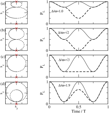
Figure 4: Time-evolution of the system in the low-frequency regime $\omega\leq\Delta$. On the left, the evolution on the Bloch sphere projected onto the $(s_{y},s_{z})$ plane. The solid line indicates the evolution of the system over the first half-period, the dotted line over the second half-period. The upper (lower) crosses indicate the states $|L\rangle$ ($|R\rangle$). On the right, the time-evolution of the probability $P_{L}(t)$ over one period of the driving. The solid line indicates zero phase-shifted driving, the dashed line has a phase-shift of $\pi/2$.

During the first and last quarter-periods of driving the time-evolution of the system is identical to that of the case with zero phase-shift, and accordingly $P_{L}(T/4)$ is given by Eq.5. It is also straightforward to show that

$$P_{L}(T/2)=\left[1-\frac{\left(\Delta/\omega\right)^{2}}{2n^{2}}\sin^{2}\pi n/2\right]^{2}.$$ (6)

In Fig.3 it can be seen that this expression indeed correctly describes the rapid fall of localization for the $\pi/2$ phase-shifted field, which reaches zero at $\Delta/\omega=\sqrt{2}$. At this value of frequency, the two rotation axes make an angle of $\pi/4$ to the $z$-axis, producing the highly symmetric time-evolution shown in Fig.4b, in which the system passes through $|R\rangle$ at $t=T/2$. As $\Delta/\omega$ is increased further, however, the trajectory of the orbit no longer passes exactly through $|R\rangle$ and thus the localization increases, producing the “revival” effect. This increase continues until $\Delta/\omega=\sqrt{3}$, at which $P_{L}(T/4)$ and $P_{L}(T/2)$ become equal. As shown in Fig.4c, at this value of frequency the system does not display any time evolution during the interval $(T/4,3T/4)$, since the action of first quarter-period of the driving is to rotate the initial state to align with $r_{-}$. The following half-period of driving under $H_{-}$, thus does not alter the state of the system.

For still larger values of $\Delta/\omega$, the rotation about the $r_{-}$ axis acts to move the system away from $|R\rangle$ (see Fig.4d), and consequently the minimum value of $P_{L}$ no longer occurs at $T/2$, but at $T/4$ instead. In this regime the localization produced by the $\pi/2$ phase-shifted field is therefore identical to that produced by the zero phase-shifted case. It can be clearly seen in Fig.3 that it is this crossover in behavior that gives rise to the revival feature seen in Fig.1.

In summary, we have studied how the CDT effect depends upon the frequency of the driving field. In the high-frequency regime, the positions of the quasienergy degeneracy can be found analytically holthaus ; creff and the degree of CDT is not affected by the phase of the driving field. As the frequency is reduced a more complicated picture appears: the quasienergies drift away from their high-frequency values along one-dimensional manifolds, and the degree of CDT induced depends not only on the values of field strength and frequency, but also on its phase. We have firstly shown that the form of the crossing-manifolds for the squarewave driving field (Eq.4) that was conjectured previously on numerical evidence creff is in fact exact. By using the Bloch sphere representation we have given a simple method of understanding how the localization falls as the frequency of the driving is reduced, and have analytically confirmed the empirical observation in Ref.bavli that the localization is maximized for zero phase-shifted driving. We have also clarified how the revival features seen for $\pi/2$ phase-shifted driving cabron arise, and have demonstrated that for crossing-manifolds with even values of $n$ that this phenomenon does not occur. This opens up new prospects for experiment in the low-frequency regime, which is both easier to attain and also has the advantage that the driving field is less likely to drive transitions to higher energy-states (thereby breaking the two-level approximation).

- (1) F. Grossmann, T. Dittrich, P. Jung and P. Hänggi, Phys. Rev. Lett. 67, 516 (1991).
- (2) M. Holthaus, Z. Phys. B: Condens. Matter 59, 251 (1992).
- (3) F. Grossmann and P. Hänggi, Europhys. Lett. 18, 571 (1992).
- (4) Jörg Lehmann, Sébastien Camalet, Sigmund Kohler and Peter Hänggi, Chem. Phys. Lett. 368, 282 (2003).
- (5) Y. Nakamura, Yu A. Pashkin and J.S. Tsai, Nature 398, 786 (1999).
- (6) D. Vion, A. Aassime, A. Cottet, P. Joyez, H. Pothier, C. Urbina, D. Esteve and M.H. Devoret, Science 296, 886 (2002).
- (7) M. Grifoni and P. Hänggi, Phys. Rep. 304, 229 (1998).
- (8) In this work we monitor the tunneling dynamics of the system continuously. If, however, the system is measured “stroboscopically” at intervals separated by the period of the driving field, CDT will always appear to be perfect if the condition of quasienergy degeneracy is satisfied.
- (9) R. Bavli and H. Metiu, Phys. Rev. Lett. 69, 1986 (1992).
- (10) J.M. Villas-Bôas, Wei Zhang, Sergio E. Ulloa, P.H. Rivera and Nelson Studart, Phys. Rev. B 66, 085325 (2002).
- (11) C.E. Creffield, Phys. Rev. B 67, 165301 (2003).
- (12) S.G. Schirmer, T. Zhang and J.V. Leahy, J. Phys. A: Math. Gen. 37, 1389 (2004).