Quantum Cluster Theories

Abstract

Quantum cluster approaches offer new perspectives to study the complexities of macroscopic correlated fermion systems. These approaches can be understood as generalized mean-field theories. Quantum cluster approaches are non-perturbative and are always in the thermodynamic limit. Their quality can be systematically improved, and they provide complementary information to finite size simulations. They have been studied intensively in recent years and are now well established. After a brief historical review, this article comparatively discusses the nature and advantages of these cluster techniques. Applications to common models of correlated electron systems are reviewed.

I Introduction

I.1 Brief history

The theoretical description of interacting many-particle systems remains one of the grand challenges in condensed matter physics. Especially the field of strongly correlated electron systems has regained theoretical and experimental interest with the discovery of heavy Fermion compounds and high-temperature superconductors. In this class of systems the strength of the interactions between particles is comparable to or larger than their kinetic energy, i.e. any theory based on a perturbative expansion around the non-interacting limit is at least questionable. Theoretical tools to describe these systems are therefore faced with extreme difficulties, due to the non-perturbative nature of the problem. A large body of work has been devoted to a direct (numerically) exact solution of finite size systems using exact diagonalization or Quantum Monte Carlo methods. Exact diagonalization however is severely limited by the exponential growth of computational effort with system size, while Quantum Monte Carlo methods suffer from the sign problem at low temperatures. Another difficulty of these methods arises from their strong finite size effects, often ruling out the reliable extraction of low energy scales that are important to capture the competition between different ground states often present in strongly correlated systems.

Mean-field theories are defined in the thermodynamic limit and therefore do not face the finite size problems. With applications to a wide variety of extended systems from spin models to models of correlated electrons and/or bosons, mean-field theories are extremely popular and ubiquitous throughout science. The first mean-field theory which gained wide acceptance was developed by P. Weiss for spin systems (Weiss, 1907). The Curie-Weiss mean-field theory reduces the complexity of the thermodynamic lattice spin problem by mapping it onto that of a magnetic impurity embedded in a self-consistently determined mean magnetic field.

Generally, mean-field theories divide the infinite number of degrees of freedom into two sets. A small set of degrees of freedom is treated explicitly, while the effects of the remaining degrees of freedom are summarized as a mean-field acting on the first set. Here, by mean-field theory, we refer to the class of approximations which account for the correlations between spatially localized degrees of freedom explicitly, while treating those at longer length scales with an effective medium. Such local approximations become exact in the limit of infinite coordination number or equivalently infinite dimensions $D$ (Itzykson and Drouffe, 1989); however non-local corrections become important in finite dimensions. The purpose of this review is to discuss methods for incorporating non-local corrections to local approximations.

Many different local approximations have been developed for systems with itinerant degrees of freedom. Early attempts focused on disordered systems, and included the virtual crystal approximation (Nordheim, 1931a, b; Parmenter, 1955; Schoen, 1969) and the average-T matrix approximation (Beeby and Edwards, 1962; Schwartz et al., 1971). However, the most successful local approximations for disordered systems is the Coherent Potential Approximation (CPA) developed by Soven (1967) and others (Taylor, 1967; Shiba, 1971). This method is distinguished from the others in that it becomes exact in both the limit of dilute and concentrated disordered impurity systems, as well as the limit of infinite dimensions.

There have been many attempts to extend the CPA formalism to correlated systems, starting with the Dynamical CPA (DCPA) of Sumi (1974); Kakehashi (2002), the XNCA of Kuramoto (1985); Kim et al. (1990) and the LNCA of Grewe (1987); Grewe et al. (1988). A great breakthrough was achieved with the formulation of the Dynamical Mean-Field Theory (DMFT) (for a review see Georges et al., 1996; Pruschke et al., 1995) in the limit of infinite dimensions by Metzner and Vollhardt (1989) and Müller-Hartmann (1989b). The DCPA and the DMFT have been the most successful approaches and employ the same mapping between the cluster and the lattice problems. They differ mostly in their starting philosophy. The DCPA employs the CPA equations to relate the impurity solution to the lattice whereas in the DMFT the irreducible quantities calculated on the impurity are used to construct the lattice quantities.

Despite the success of these mean-field approaches, they share the critical flaw of neglecting the effects of non-local fluctuations. Thus they are unable to capture the physics of, e.g. spin waves in spin systems, localization in disordered systems, or spin-liquid physics in correlated electronic systems. Non-local corrections are required to treat even the initial effects of these phenomena and to describe phase transitions to states described by a non-local order parameter.

The first attempt to add non-local corrections to mean-field theories was due to Bethe (1935) by adding corrections to the Curie-Weiss mean-field theory. This was achieved by mapping the lattice problem onto a self-consistently embedded finite-size spin cluster composed of a central site and $z$ nearest neighbors embedded in a mean-field. For small $z$, the resulting theory provides a remarkably large and accurate correction to the transition temperature (Kikuchi, 1951; Suzuki, 1986).

Many attempts have been made to apply similar ideas to disordered electronic systems (Gonis, 1992). Most approaches were hampered by the difficulty of constructing a fully causal theory, with positive spectral functions. Several causal theories were developed including the embedded cluster method (Gonis, 1992) and the molecular CPA (MCPA) by Tsukada (1969) (for a review see Ducastelle, 1974). These methods generally are obtained from the local approximation by replacing the impurity by a finite size cluster in real space. As a result these approaches suffer from the lack of translational invariance, since the cluster has open boundary conditions and only the surface sites couple to the mean-field.

Similar effort has been expended to find cluster extensions to the DMFT, including most notably the Dynamical Cluster Approximation (DCA) (Hettler et al., 1998, 2000) and the Cellular Dynamical Mean-Field Theory (CDMFT) (Kotliar et al., 2001). Both cluster approaches reduce the complexity of the lattice problem by mapping it to a finite size cluster self-consistently embedded in a mean-field. As in the classical case, the self-consistency condition reflects the translationally invariant nature of the original lattice problem. The main difference with their classical counterparts arises from the presence of quantum fluctuations. Mean-field theories for quantum systems with itinerant degrees of freedom cut off spatial fluctuations but take full account of temporal fluctuations. As a result the mean-field is a time- or respectively frequency dependent quantity. Even an effective cluster problem consisting of only a single site (DMFT) is hence a highly non-trivial many-body problem. CDMFT and DCA mainly differ in the nature of the effective cluster problem. The CDMFT shares an identical mapping of the lattice to the cluster problem with the MCPA, and hence also violates translational symmetries on the cluster. The DCA maps the lattice to a periodic and therefore translationally invariant cluster.

A numerically more tractable cluster approximation to the thermodynamic limit was developed by Gros and Valenti (1994). In this formalism the self-consistent coupling to a mean-field is neglected. This leads to a theory in which the self-energy of an isolated finite size cluster is used to approximate the lattice propagator. As shown by Sénéchal et al. (2000), this cluster extension of the Hubbard-I approximation is obtained as the leading order approximation in a strong-coupling expansion in the hopping amplitude and hence this method was named Cluster Perturbation Theory (CPT).

Generally, cluster formalisms share the basic idea to approximate the effects of correlations in the infinite lattice problem with those on a finite size quantum cluster. We refer to this class of techniques as quantum cluster theories. In contrast to Finite System Simulations (FSS), these techniques are built for the thermodynamic limit. In this review we focus on the three most established quantum cluster approaches, the DCA, the CDMFT and the CPT formalisms. The CDMFT approach was originally formulated for general, possibly non-orthogonal basis sets. In this review we restrict the discussion to the usual, completely localized orthogonal basis set and refer the reader to Kotliar et al. (2001) for the generalization to arbitrary basis sets.

The organization of this article is as follows: To familiarize the reader with the concept of cluster approaches, we develop in section I.2 a cluster generalization of the Curie-Weiss mean-field theory for spin systems. Section II sets up the theoretical framework of the CDMFT, DCA and CPT formalisms by presenting two derivations based on different starting philosophies. The derivation based on the locator expansion in Sec. II.1 is analogous to the cluster generalization of the Curie-Weiss mean-field method and thus is physically very intuitive. The derivation based on the cluster approximation to diagrams defining the grand potential in Sec. II.2 is closely related to the reciprocal space derivation of the DMFT by Müller-Hartmann (1989b). The nature of the different quantum cluster approaches together with their advantages and weaknesses are assessed in Sec. II.3. Discussions of the effective cluster problem, generalizations to symmetry broken states and the calculation of response functions are presented in Secs. II.4, II.5 and II.6. The remainder of this section is devoted to describe the application of the DCA formalism to disordered systems in Sec. II.7 and to a brief discussion of alternative methods proposed to introduce non-local corrections to the DMFT method in Sec. II.8. In Sec. III we review the various perturbative and non-perturbative techniques available to solve the effective self-consistent cluster problem of quantum cluster approaches. We include a detailed assessment of their advantages and limitations. Although numerous applications of quantum cluster approaches to models of many-particle systems are found in the literature, this field is still in its footsteps and currently very active. A large body of work has been concentrated on the Hubbard model. We review the progress made on this model in Section IV together with applications to several other strongly correlated models. Finally, Sec. V concludes the review by stressing the limitations of quantum cluster approaches and proposing possible directions for future research in this field.

I.2 Corrections to Curie-Weiss theory

As an intuitive example of the formalism developed in the next sections we consider a systematic cluster extension of the Curie-Weiss mean-field theory for a lattice of classical interacting spins. This discussion is especially helpful to illustrate many new aspects of cluster approaches as compared to finite size simulations. The quality of this approach, and its convergence and critical properties will be demonstrated with a simple example, the one-dimensional Ising model

$$H=-J\sum_{i}\sigma_{i}\sigma_{i+1}-h\sum_{i}\sigma_{i}$$ (1)

where $\sigma_{i}=\pm 1$ are classical spins, $h$ is an external magnetic field and the exchange integral $J>0$ acts between nearest neighbors only, favoring ferromagnetism. The generalization of this approach to higher dimensions and quantum spin systems is straightforward.

We start by dividing the infinite lattice into $N/N_{c}$ clusters of size $N_{c}$ (see Fig. 3) with origin ${\tilde{x}}$ and the exchange integral $J_{ij}$ into intra- (${\bf J}_{c}$) and inter-cluster ($\delta{\bf J}$) parts

$${\bf J}({\tilde{x}}_{i}-{\tilde{x}}_{j})={\bf J}_{c}\delta_{{\tilde{x}}_{i},{\tilde{x}}_{j}}+\delta{\bf J}({\tilde{x}}_{i}-{\tilde{x}}_{j})$$ (2)

where each of the terms is a matrix in the $N_{c}$ cluster sites. The central approximation of cluster theories is to retain correlation effects within the cluster and neglect them between the clusters. A natural formalism to implement this approximation is the locator expansion. The spin-susceptibility $\chi_{ij}=\beta(\langle\sigma_{i}\sigma_{j}\rangle-\langle\sigma_{i}\rangle\langle\sigma_{j}\rangle)$, where $\beta=1/T$ is the inverse temperature, can be written as a locator expansion in the inter-cluster part $\delta{\bf J}$ of the exchange interaction, around the cluster limit ${\boldsymbol{\chi}}^{o}={\boldsymbol{\chi}}(\delta{\bf J}=0)$ as

$${\boldsymbol{\chi}}({\tilde{x}}_{i}-{\tilde{x}}_{j})={\boldsymbol{\chi}}^{o}\delta_{{\tilde{x}}_{i},{\tilde{x}}_{j}}+{\boldsymbol{\chi}}^{o}\sum_{l}\delta{\bf J}({\tilde{x}}_{i}-{\tilde{x}}_{l}){\boldsymbol{\chi}}({\tilde{x}}_{l}-{\tilde{x}}_{j})$$ (3)

where we used again a matrix notation in the $N_{c}$ cluster sites. By using the translational invariance of quantities in the superlattice ${\tilde{x}}$, this expression can be simplified in the reciprocal space ${\tilde{q}}$ of ${\tilde{x}}$ to

$${\boldsymbol{\chi}}({\tilde{q}})={\boldsymbol{\chi}}^{o}+{\boldsymbol{\chi}}^{o}\delta{\bf J}({\tilde{q}}){\boldsymbol{\chi}}({\tilde{q}})\,.$$ (4)

This locator expansion has two well-defined limits. For an infinite size cluster it recovers the exact result since the surface to volume ratio vanishes making $\delta{\bf J}$ irrelevant, and thus ${\boldsymbol{\chi}}={\boldsymbol{\chi}}^{o}$. For a single site cluster, $N_{c}=1$, it recovers the Curie-Weiss mean-field theory. This is intuitively clear since for $N_{c}=1$ fluctuations between all sites are neglected. With the susceptibility of a single isolated site $\chi^{o}=1/T$ and $\delta J({\tilde{q}}=0)=J(q=0)=J$, we obtain for the uniform susceptibility

$$\chi(q=0)=\frac{1}{1/\chi^{o}-J(q=0)}=\frac{1}{T-T_{c}}$$ (5)

the mean-field result with critical temperature $T_{c}=J$.

For cluster sizes larger than one, translational symmetry within the cluster is violated since the clusters have open boundary conditions and $\delta{\bf J}$ only couples sites on the surface of the clusters. As detailed in the next section, this shortcoming can be formally overcome and translational invariance restored by considering an analogous expression to the locator expansion (4) in the Fourier space $Q$ of the cluster

$$\chi(Q,{\tilde{q}}) = \chi^{o}(Q)+\chi^{o}(Q)\delta J(Q,{\tilde{q}})\chi(Q,{\tilde{q}})$$ (6)

$$= \frac{1}{1/{\chi^{o}}(Q)-\delta J(Q,{\tilde{q}})}\,,$$

with analogous relations for the intra- and inter-cluster parts of $J$

$$\delta J(Q,{\tilde{q}}) = J(Q+{\tilde{q}})-{\bar{J}}(Q)$$ (7)

$${\bar{J}}(Q) = \frac{N_{c}}{N}\sum_{\tilde{q}}J(Q+{\tilde{q}})\,.$$ (8)

Here, ${\tilde{q}}$ is a vector in the reciprocal space of ${\tilde{x}}$, and $Q$ is a vector in the reciprocal space of the cluster sites. The Fourier transform of the exchange integral is given by $J(Q+{\tilde{q}})=J\cos(Q+{\tilde{q}})$, the intra-cluster exchange is $\bar{J}(Q)$, while the inter-cluster exchange is $\delta J(Q,{\tilde{q}})$. As we will see in the next section, the resulting formalism is analogous to the dynamical cluster approximation for itinerant fermion systems.

In analogy to the Curie-Weiss theory, the lattice system can now be mapped onto an effective cluster model embedded in a mean-field since correlations between the clusters are neglected. The susceptibility restricted to cluster sites is obtained by averaging or coarse-graining over the superlattice wave-vectors ${\tilde{q}}$

$${\bar{\chi}}(Q)=\frac{N_{c}}{N}\sum_{{\tilde{q}}}\chi(Q,{\tilde{q}})=\frac{1}{1/\chi^{o}(Q)-\Gamma(Q)}\,.$$ (9)

with the hybridization function

$$\Gamma(Q)=\frac{\frac{N_{c}}{N}\sum_{\tilde{q}}\delta J^{2}(Q,{\tilde{q}})\chi(Q,{\tilde{q}})}{1+\frac{N_{c}}{N}\sum_{\tilde{q}}\delta J(Q,{\tilde{q}})\chi(Q,{\tilde{q}})}\,.$$ (10)

This follows from the fact that the isolated cluster susceptibility $\chi^{o}(Q)$ does not depend on the integration variable ${\tilde{q}}$ in Eq. (9).

This expression defines the effective cluster model

$${\cal H}_{c} = -\sum_{Q}{\bar{J}}(Q)\sigma(Q)\sigma(-Q)-h\sigma(Q=0)$$ (11)

$$-\sum_{Q,{\tilde{q}}}\delta J(Q,{\tilde{q}})\sigma(Q)\langle\sigma(-Q-{\tilde{q}})\rangle\,,$$

where $\sigma(Q)$ ($\sigma(q)$) denotes the cluster (lattice) Fourier transform of $\sigma_{i}$ and $\langle\dots\rangle$ the expectation value calculated with respect to the cluster Hamiltonian ${\cal H}_{c}$. As in the Curie-Weiss theory, the cluster model is used to self-consistently determine the order parameter $\langle\sigma(Q+{\tilde{q}})\rangle=\langle\sigma(Q)\rangle\delta({\tilde{q}})$ in the ferromagnetic state. In the paramagnetic state, the susceptibility calculated in the cluster model takes the same form as the coarse-grained result Eq. (9) obtained from the locator expansion.

The uniform susceptibility $\chi(Q=0,{\tilde{q}}=0)$ contains information about the nature of this cluster approach, its critical properties and its convergence with cluster size. The sum in Eq. (8) may be solved analytically

$${\bar{J}}(Q=0)=J(N_{c}/\pi)\sin(\pi/N_{c})\,.$$ (12)

The isolated cluster susceptibility $\chi^{o}(Q)$ can also be calculated analytically by using the transfer matrix method to give Goldenfeld (1992)

$$\chi^{o}(Q=0)=\beta\exp(2K)\frac{1-\left(\tanh(K)\right)^{N_{c}}}{1+\left(\tanh(K)\right)^{N_{c}}}\,,$$ (13)

where $K=\beta{\bar{J}}(Q=0)=\beta J(N_{c}/\pi)\sin(\pi/N_{c})$. With these expressions the uniform lattice susceptibility Eq. (6) becomes

$$\chi(T) = \frac{1}{1/\chi^{o}(Q=0)-\delta J(Q=0,{\tilde{q}}=0)}$$

$$= \frac{1}{1/\chi^{o}(Q=0)-J\left(1-(N_{c}/\pi)\sin(\pi/N_{c})\right)}\,.$$

The cluster estimate of the lattice susceptibility interpolates between the Curie-Weiss result and the exact lattice result as $N_{c}$ increases. It may be used to reveal some of the properties of cluster approximations and to compare the cluster results to both the finite-size calculation and the exact result in the thermodynamic limit.

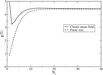
Figure 1: The cluster and finite-size estimates of the uniform lattice susceptibility versus cluster size when $J=1$ and $T=0.7$.

First, both the cluster mean-field result Eq. (I.2) and the finite-size result Eq. (13) with $K=\beta J$ may be regarded as an approximation to the thermodynamic result. However, as illustrated in Fig. 1, the cluster mean-field result converges more quickly as a function of cluster size $N_{c}$ than the finite size result. This reflects the superior starting point of the cluster approximation compared to the finite-size calculation. The cluster approximation is an expansion about the mean-field result, whereas the finite-size calculation is an expansion about the atomic limit.

It is instructive to explore the convergence of the cluster result analytically. For large $N_{c}$, the character of the susceptibility Eq. (I.2) can be split into three regimes. At very high temperatures

$$\chi(T)\approx\frac{1}{T-\Theta}\;\;\;{\mbox{for}}\;\;\;T\gg J$$ (15)

where $\Theta\approx 2J+\frac{J}{6}\left(\frac{\pi}{N_{c}}\right)^{2}$. At intermediate temperatures,

$$\chi(T)\approx\beta e^{2\beta J}\left(1-\frac{\beta J}{3}\left(\frac{\pi}{N_{c}}\right)^{2}\right)\;\;\;{\mbox{for}}\;\;\;J\gg T\gg T_{c}\,.$$ (16)

The true critical behavior of the system can be resolved by studying the properties of this intermediate temperature regime. At both high and intermediate temperatures, the susceptibility differs from the exact result by corrections of order ${\cal{O}}(1/N_{c}^{2})$. In general, cluster methods with periodic boundary conditions have corrections of order ${\cal{O}}(1/L_{c}^{2})$, where $L_{c}=N_{c}^{1/D}$ is the linear size of the cluster.

At low temperatures, very close to the transition to the ferromagnetic state, deviations from the exact result are far larger. Here, for large clusters

$$\chi(T)\sim\frac{N_{c}}{T-T_{c}}\,,$$ (17)

with the critical temperature $T_{c}>0$, whereas the exact susceptibility in this regime $\chi(T)\approx\beta\exp{\left(2\beta J\right)}$ does not diverge until zero temperature. This discrepancy is expected in cluster approximations, since they treat long length scales which drive the transition in a mean-field way and therefore neglect long wave-length modes which eventually suppress the transition. Hence, cluster approximations generally predict finite transition temperatures independent of dimensionality due to their residual mean-field character. With increasing cluster size however, the transitions are expected to be systematically suppressed by the inclusion of longer-ranged fluctuations.

For cluster sizes larger than one, all three regions are evident in the plot of the cluster mean-field estimate of the inverse susceptibility, shown in the inset to Fig. 2. For $N_{c}=8$ and $N_{c}=16$, the high and low temperature parts are seen as straight lines on the plot in the inset, with the crossover region in between. In numerical simulations with significant sources of numerical noise especially close to the transition, it is extremely difficult to resolve the true low-temperature mean-field behavior. Exponents extracted from fits to the susceptibility in these simulations will more likely reflect the properties of the intermediate temperature regime.

Despite the large deviations of the cluster result from the exact result low temperatures, we may still extract the correct physics through finite size extrapolation. In general, for a system where the correlations build like $\xi\sim\left|\frac{T-T_{c}}{T_{c}}\right|^{-\nu}$, we expect $T_{c}\sim T_{c}^{*}-aL_{c}^{-1/\nu}$, where $T_{c}^{*}$ is the exact transition temperature, $L_{c}$ is the linear cluster size, and $a$ is a positive real constant Suzuki (1986). However, for the 1D Ising system, $\xi\sim\frac{1}{2}\exp{\left(\beta J\right)}$, so more care must be taken. Fortunately, an analytic expression for the transition temperature may be extracted from Eq. (I.2). For large clusters, $T_{c}\approx JN_{c}\left(\frac{1}{6}\left(\frac{\pi}{N_{c}}\right)^{2}-\frac{1}{120}\left(\frac{\pi}{N_{c}}\right)^{4}\right)$. This behavior is shown in the main frame of Fig. 2 with the circles depicting the numerical values for $T_{c}$ and the solid line their asymptotic behavior.

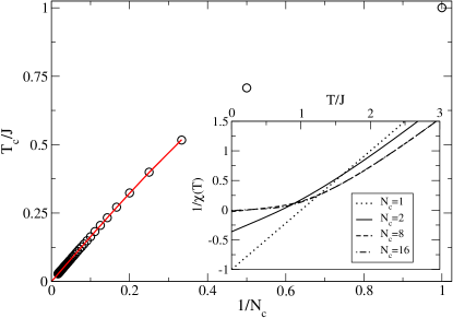
Figure 2: Transition temperature for the 1D Ising model versus the inverse cluster size when $J=1$ obtained with the cluster mean-field approach. For large clusters, $T_{c}\sim 1/N_{c}$, shown as a solid line. Inset: The inverse susceptibility versus temperature. The Curie-Weiss behavior at low $T$ where $1/\chi(T)$ is linear in $T$, illustrates that the transition is always mean-field like. The true critical behavior of the transition is seen in the crossover region near $T=J$.

II Quantum cluster theories

In this section we provide two derivations of quantum cluster approaches for systems with itinerant quantum degrees of freedom. The locator expansion in Sec. II.1 is analogous to the cluster extension of the Curie-Weiss mean-field theory developed in the preceding section. Sec. II.2 provides a microscopic derivation based on cluster approximations to the thermodynamic grand potential. A detailed discussion of the nature of quantum cluster approaches and the effective cluster model is presented in Secs. II.3 and II.4. Generalizations for symmetry broken phases, the calculation of susceptibilities and the application to disordered systems is explained in Secs. II.5, II.6 and II.7 and a brief discussion of alternative cluster methods is presented in Sec. II.8.

II.1 Cluster approximation to the locator expansion

In this section, we derive a number of cluster formalisms for itinerant many body systems using an analogous approach to that discussed in Sec. I.2 for classical spin systems. For simplicity we assume in this section that no symmetry breaking occurs; the treatment of symmetry broken phases is discussed in Sec. II.5. The basic idea is to write down a locator expansion, i.e. an expansion in space around a finite-size cluster. This approach is not only intuitive but also allows us to assess the nature of quantum cluster approximations. As with their classical counterparts, quantum cluster theories approximate the lattice problem with many degrees of freedom by an effective cluster problem with few degrees of freedom embedded in an external bath or mean-field created from the remaining degrees of freedom. By neglecting correlations that extend beyond the cluster size, one can then formulate a theory in which the lattice system is replaced by an effective cluster embedded in a mean-field host. While the formalism derived here is analogous to the formalism discussed in Sec. I.2 for spin systems, there are significant differences. Since we are dealing with itinerant fermions, the theory is built upon the single-particle Green function instead of the two-particle spin correlation function, and the mean-field is dynamical due to the itinerant nature of the particles.

This derivation is illustrated on the example of the extended Hubbard model

$$H=\sum_{ij,\sigma}t_{ij}c^{\dagger}_{i\sigma}c_{j\sigma}+\frac{1}{2}\sum_{ij,\sigma\sigma^{\prime}}U_{ij}n_{i\sigma}n_{j\sigma^{\prime}}\,.$$ (18)

Here $i$ and $j$ are lattice site indices, the operators $c_{i\sigma}^{\dagger}$ ($c_{i\sigma}$) create (destroy) an electron with spin $\sigma$ on site $i$, $n_{i\sigma}=c^{\dagger}_{i\sigma}c_{i\sigma}$ is their corresponding number density, and $U_{ij}$ denotes the Coulomb repulsion between electrons on sites $i$ and $j$. The hopping amplitude between sites $i$ and $j$ is denoted by $t_{ij}$, its local contribution $t_{ii}=\epsilon_{o}$ and its Fourier transform to reciprocal space is the dispersion $\epsilon_{\bf{k}}$. In this section we limit the discussion to the regular Hubbard model with a purely local interaction $U_{ij}=U(1-\delta_{\sigma\sigma^{\prime}})\delta_{ij}$. The more general case of finite non-local interactions $U_{ij}$ for $i\neq j$ is discussed in Sec. II.2.

The central quantity upon which we build the locator expansion is the single-particle thermodynamic Green function ($\tau$ is the imaginary time, $T_{\tau}$ the corresponding time ordering operator, $\beta=1/T$ the inverse temperature and $\omega_{n}$ are the fermionic Matsubara frequencies)

$$G_{ij,\sigma}(\tau)=-\langle T_{\tau}c_{i\sigma}(\tau)c^{\dagger}_{j\sigma}\rangle$$ (19)

$$G_{ij,\sigma}(i\omega_{n})=\int\limits_{0}^{\beta}d\tau e^{i\omega_{n}\tau}G_{ij,\sigma}(\tau)\,;\,\,\omega_{n}=\frac{(2n+1)\pi}{\beta}$$ (20)

or respectively its analytical continuation $G_{ij,\sigma}(z)=\langle\langle c_{i\sigma},c^{\dagger}_{j\sigma}\rangle\rangle_{z}$ to complex frequencies $z$.

To set up a suitable notation for cluster schemes, we divide the $D$-dimensional lattice of $N$ sites into a set of finite-size clusters each with $N_{c}$ sites of linear size $L_{c}$ such that $N_{c}=L_{c}^{D}$, and resolve the first Brillouin zone into a corresponding set of reduced zones which we call cells. This notation is illustrated in Fig. 3 for $N_{c}=4$ site clusters. For larger cluster sizes and more complex cluster geometries we refer the reader to Jarrell et al. (2001b). Care should be taken so that the point group symmetry of the clusters does not differ too greatly from that of the original lattice Betts and Stewart (1997). We use the coordinate ${\tilde{{\bf x}}}$ to label the origin of the clusters and ${\bf X}$ to label the $N_{c}$ sites within a cluster, so that the site indices of the original lattice ${\bf x}={\bf X}+{\tilde{{\bf x}}}$. The points ${\tilde{{\bf x}}}$ form a superlattice with a reciprocal space labeled by ${\tilde{{\bf{k}}}}$. The reciprocal space corresponding to the sites ${\bf X}$ within a cluster shall be labeled ${\bf{K}}$, with $K_{\alpha}=n_{\alpha}\cdot 2\pi/L_{c}$ and integer $n_{\alpha}$. Then the wave-vectors in the full Brillouin zone are given by ${\bf{k}}={\bf{K}}+{\tilde{{\bf{k}}}}$.

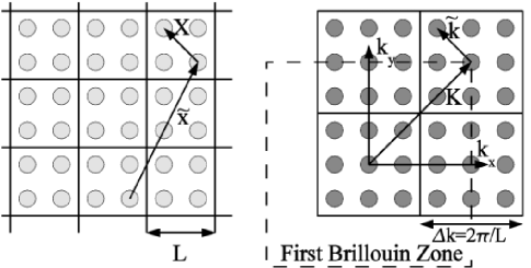
Figure 3: Definition of the coordinates in real (left) and reciprocal (right) space illustrated for $N_{c}=4$ site clusters. The origin of a cluster is labeled by ${\tilde{{\bf x}}}$, the sites within a cluster by ${\bf X}$. The reciprocal space to ${\bf X}$ is labeled by ${\bf{K}}$, the wave-vectors of the superlattice, i.e. within a cell by ${\tilde{{\bf{k}}}}$.

With these conventions, the Fourier transforms of a given function $f({\bf X},{\tilde{{\bf x}}})$ for intra- and inter-cluster coordinates are defined as

$$f({\bf X},{\tilde{{\bf x}}}) = \frac{N_{c}}{N}\sum_{\tilde{{\bf{k}}}}e^{i{\tilde{{\bf{k}}}}\cdot{\tilde{{\bf x}}}}f({\bf X},{\tilde{{\bf{k}}}})$$ (21)

$$f({\bf X},{\tilde{{\bf{k}}}}) = \sum_{\tilde{{\bf x}}}e^{-i{\tilde{{\bf{k}}}}\cdot{\tilde{{\bf x}}}}f({\bf X},{\tilde{{\bf x}}})$$ (22)

$$f({\bf X},{\tilde{{\bf{k}}}}) = \frac{1}{N_{c}}\sum_{\bf{K}}e^{i({\bf{K}}+{\tilde{{\bf{k}}}})\cdot{\bf X}}f({\bf{K}},{\tilde{{\bf{k}}}})$$ (23)

$$f({\bf{K}},{\tilde{{\bf{k}}}}) = \sum_{\bf X}e^{-i({\bf{K}}+{\tilde{{\bf{k}}}})\cdot{\bf X}}f({\bf X},{\tilde{{\bf{k}}}})\,.$$ (24)

To separate out the cluster degrees of freedom, the hopping amplitude $t$ and the self-energy $\Sigma$ (defined from the Green function via the Dyson equation $G^{-1}=G_{0}^{-1}-\Sigma$ with the non-interacting Green function $G_{0}$) is split into intra- and inter-cluster parts

$${\bf t}({\tilde{{\bf x}}}_{i}-{\tilde{{\bf x}}}_{j}) = {\bf t}_{c}\delta_{{\tilde{{\bf x}}}_{i},{\tilde{{\bf x}}}_{j}}+\delta{\bf t}({\tilde{{\bf x}}}_{i}-{\tilde{{\bf x}}}_{j})$$ (25)

$${\bf\Sigma}({\tilde{{\bf x}}}_{i}-{\tilde{{\bf x}}}_{j},z) = {\bf\Sigma}_{c}(z)\delta_{{\tilde{{\bf x}}}_{i},{\tilde{{\bf x}}}_{j}}+\delta{\bf\Sigma}({\tilde{{\bf x}}}_{i}-{\tilde{{\bf x}}}_{j},z)\,.$$ (26)

All the quantities are $N_{c}\times N_{c}$ matrices in the cluster sites, ${\bf t}_{c}={\bf t}({\tilde{{\bf x}}}=0)$ and ${\bf\Sigma}_{c}(z)={\bf\Sigma}({\tilde{{\bf x}}}=0,z)$ are the intra-cluster hopping and self-energy, while $\delta{\bf t}({\tilde{{\bf x}}})$ and $\delta{\bf\Sigma}({\tilde{{\bf x}}},z)$ are the corresponding inter-cluster quantities only finite for ${\tilde{{\bf x}}}\neq 0$.

With these definitions we write the Green function using a locator expansion, an expansion in $\delta{\bf t}$ and $\delta{\bf\Sigma}$ around the cluster limit. In matrix notation in the $N_{c}$ cluster sites it reads

$${\bf G}({\tilde{{\bf x}}}_{i}-{\tilde{{\bf x}}}_{j},z) = {\bf g}(z)\delta_{{\tilde{{\bf x}}}_{i}{\tilde{{\bf x}}}_{j}}+{\bf g}(z)\sum_{l}[\delta{\bf t}({\tilde{{\bf x}}}_{i}-{\tilde{{\bf x}}}_{l})$$ (27)

$$+ \delta{\bf\Sigma}({\tilde{{\bf x}}}_{i}-{\tilde{{\bf x}}}_{l},z)]{\bf G}({\tilde{{\bf x}}}_{l}-{\tilde{{\bf x}}}_{j},z)$$

where the $N_{c}\times N_{c}$ matrix

$${\bf g}(z)=[(z+\mu)\mathbb{1}-{\bf t}_{c}-{\bf\Sigma}_{c}(z)]^{-1}$$ (28)

is the Green function of the cluster decoupled from the remainder of the system ($\mu$ is the chemical potential). Since translational invariance in the superlattice ${\tilde{{\bf x}}}$ is preserved, this expression may be simplified by Fourier transforming the inter-cluster coordinates to give

$${\bf G}({\tilde{{\bf{k}}}},z)={\bf g}(z)+{\bf g}(z)[\delta{\bf t}({\tilde{{\bf{k}}}})+\delta{\bf\Sigma}({\tilde{{\bf{k}}}},z)]{\bf G}({\tilde{{\bf{k}}}},z)\,.$$ (29)

The central approximation that unites all cluster formalisms is to truncate the self-energy to the cluster, by neglecting $\delta{\bf\Sigma}$ to arrive at

$${\bf G}({\tilde{{\bf{k}}}},z) = {\bf g}(z)+{\bf g}(z)\delta{\bf t}({\tilde{{\bf{k}}}}){\bf G}({\tilde{{\bf{k}}}},z)$$ (30)

$$= [{\bf g}^{-1}(z)-\delta{\bf t}({\tilde{{\bf{k}}}})]^{-1}\,.$$

As we discuss below, this approximation corresponds to truncating the potential energy to the cluster while keeping all the contributions to the kinetic energy. Therefore quantum cluster approaches are good approximations to systems with significant screening, where non-local correlations are expected to be short-ranged. Quantum cluster approaches are particularly powerful because the remaining self-energy term ${\bf\Sigma}_{c}(z)$ implicitly contained in the propagator ${\bf g}(z)$ in Eq. (30) is restricted to the cluster degrees of freedom. Hence it can be calculated non-perturbatively in an effective cluster model as a functional ${\bf\Sigma}_{c}(z)={\cal F}[\bar{\bf G}(z)]$, where

$$\bar{\bf G}(z)=\frac{N_{c}}{N}\sum_{{\tilde{{\bf{k}}}}}{\bf G}({\tilde{{\bf{k}}}},z)$$ (31)

is the ${\tilde{{\bf{k}}}}$-averaged or coarse-grained ${\bf G}({\tilde{{\bf{k}}}},z)$, i.e. the Green function restricted to the cluster. As discussed in the next section this approximation is consistent with neglecting inter-cluster momentum conservation, i.e. neglecting the phase factors $e^{i{\tilde{{\bf{k}}}}\cdot{\tilde{{\bf x}}}}$ on the vertices of the self-energy diagrams.

Using the expression (30) for the lattice Green function and the fact that ${\bf g}(z)$ does not depend on ${\tilde{{\bf{k}}}}$, the coarse-grained Green function $\bar{\bf G}$ can be written as

$$\bar{\bf G}(z)=[{\bf g}^{-1}(z)-{\bf\Gamma}(z)]^{-1}\;\;,$$ (32)

with a hybridization function ${\bf\Gamma}$ defined by

$${\bf\Gamma}(z) = \left[\mathbb{1}+\frac{N_{c}}{N}\sum_{\tilde{{\bf{k}}}}\delta{\bf t}({\tilde{{\bf{k}}}}){\bf G}({\tilde{{\bf{k}}}},z)\right]^{-1}$$ (33)

$$\times \left[\frac{N_{c}}{N}\sum_{{\tilde{{\bf{k}}}}}\delta{\bf t}({\tilde{{\bf{k}}}}){\bf G}({\tilde{{\bf{k}}}},z)\delta{\bf t}({\tilde{{\bf{k}}}})\right]\,.$$

Its physical content is that of an effective amplitude for fermionic hopping processes from the cluster into the host and back again into the cluster. The denominator in Eq. (33) is a correction that excludes the cluster from the effective medium. ${\bf\Gamma}(z)$ thus plays an analogous role to that of the internal magnetic field in mean-field approximations of spin systems. However, due to the itinerant character of the fermionic degrees of freedom, it is a dynamical quantity.

Both the CPT and the CDMFT formalisms may be defined at this point. A self-consistent set of equations is formed from ${\bf G}$ as a functional of ${\bf\Sigma}_{c}$ using Eq. (30) together with Eq. (28), and with an appropriate choice of a cluster solver (see Sec. III), ${\bf\Sigma}_{c}$ as a functional of $\bar{\bf G}$. In the CDMFT approximation the hybridization ${\bf\Gamma}$ is determined self-consistently with Eq. (33), i.e. from the translational invariance of the super-lattice. The resulting self-consistency cycle is discussed in Sec. II.2.4. The CPT formalism is obtained when ${\bf\Gamma}$ is neglected. The Green function ${\bf g}(z)$ then becomes the Green function of an isolated cluster and the CPT result for the lattice Green function is obtained immediately via Eq. (30) without self-consistency. Thus the renormalization of the cluster degrees of freedom due to the coupling to the host described by ${\bf\Gamma}$ is neglected in the CPT but included in the CDMFT formalism.

The DCA formalism may be motivated by the demand to restore translational invariance within the cluster. Since the inter-cluster hopping $\delta{\bf t}({\tilde{{\bf{k}}}})$ is finite for sites on the surface of the cluster and zero for bulk sites, only surface sites hybridize with the host. Hence translational invariance with respect to the cluster sites ${\bf X}$ is violated. The cause of this violation can be seen by representing the hopping integral ${\bf t}({\tilde{{\bf{k}}}})$ as the intra-cluster Fourier transform of the dispersion $\epsilon_{{\bf{K}}+{\tilde{{\bf{k}}}}}$ using Eq. (23),

$$[{\bf t}({\tilde{{\bf{k}}}})]_{{\bf X}_{i}{\bf X}_{j}}=\frac{1}{N_{c}}\sum_{\bf{K}}e^{i({\bf{K}}+{\tilde{{\bf{k}}}})\cdot({\bf X}_{i}-{\bf X}_{j})}\epsilon_{{\bf{K}}+{\tilde{{\bf{k}}}}}\,.$$ (34)

The violation of translational symmetry is caused by the phase factors $e^{i{\tilde{{\bf{k}}}}\cdot({\bf X}_{i}-{\bf X}_{j})}$ associated with the superlattice wave-vectors ${\tilde{{\bf{k}}}}$. Thus translational symmetry can be restored by neglecting these phase-factors, or equivalently, by multiplying $[{\bf t}({\tilde{{\bf{k}}}})]_{{\bf X}_{i}{\bf X}_{j}}$ with the ${\tilde{{\bf{k}}}}$-dependent phase $e^{-i{\tilde{{\bf{k}}}}\cdot({\bf X}_{i}-{\bf X}_{j})}$,

$$[{\bf t}_{DCA}({\tilde{{\bf{k}}}})]_{{\bf X}_{i}{\bf X}_{j}} = [{\bf t}({\tilde{{\bf{k}}}})]_{{\bf X}_{i}{\bf X}_{j}}e^{-i{\tilde{{\bf{k}}}}\cdot({\bf X}_{i}-{\bf X}_{j})}$$ (35)

$$= \frac{1}{N_{c}}\sum_{{\bf{K}}}e^{i{\bf{K}}\cdot({\bf X}_{i}-{\bf X}_{j})}\epsilon_{{\bf{K}}+{\tilde{{\bf{k}}}}}\,.$$

Since ${\bf t}_{DCA}$ is fully cyclic in the cluster sites, the DCA intra- and inter-cluster hopping integrals can be written as cluster Fourier transforms

$$[{\bf t}_{c,DCA}]_{{\bf X}_{i}{\bf X}_{j}} = \frac{1}{N_{c}}\sum_{\bf{K}}e^{i{\bf{K}}\cdot({\bf X}_{i}-{\bf X}_{j})}\bar{\epsilon}_{\bf{K}}$$ (36)

$$\left[\delta{\bf t}_{DCA}({\tilde{{\bf{k}}}})\right]_{{\bf X}_{i}{\bf X}_{j}} = \frac{1}{N_{c}}\sum_{\bf{K}}e^{i{\bf{K}}\cdot({\bf X}_{i}-{\bf X}_{j})}\delta t({\bf{K}}+{\tilde{{\bf{k}}}})$$ (37)

with

$$\bar{\epsilon}_{\bf{K}} = \frac{N_{c}}{N}\sum_{\tilde{{\bf{k}}}}\epsilon_{{\bf{K}}+{\tilde{{\bf{k}}}}}$$ (38)

$$\delta t({\bf{K}}+{\tilde{{\bf{k}}}}) = \epsilon_{{\bf{K}}+{\tilde{{\bf{k}}}}}-\bar{\epsilon}_{\bf{K}}\,.$$ (39)

Since the DCA intra- and inter-cluster hopping integrals retain translational invariance within the cluster, the DCA cluster self-energy ${\bf\Sigma}_{c}$ and hybridization function ${\bf\Gamma}$ are translationally invariant. The lattice Green function, Eq. (30) hence becomes diagonal in cluster Fourier space

$$G({\bf{K}}+{\tilde{{\bf{k}}}},z) = g({\bf{K}},z)+g({\bf{K}},z)\delta t({\bf{K}}+{\tilde{{\bf{k}}}})G({\bf{K}}+{\tilde{{\bf{k}}}},z)$$ (40)

$$= \frac{1}{g^{-1}({\bf{K}},z)-\delta t({\bf{K}}+{\tilde{{\bf{k}}}})}$$

with the Green function decoupled from the host

$$g({\bf{K}},z)=[z-\bar{\epsilon}_{\bf{K}}+\mu-\Sigma_{c}({\bf{K}},z)]^{-1}\,.$$ (41)

Along the lines presented above, the DCA cluster self-energy $\Sigma_{c}({\bf{K}},z)$ is calculated as a functional of the coarse-grained Green function

$$\bar{G}({\bf{K}},z) = \frac{N_{c}}{N}\sum_{\tilde{{\bf{k}}}}G({\bf{K}}+{\tilde{{\bf{k}}}},z)$$ (42)

$$= \frac{1}{g^{-1}({\bf{K}},z)-\Gamma({\bf{K}},z)}$$

which defines the DCA hybridization function

$$\Gamma({\bf{K}},z)=\frac{\frac{N_{c}}{N}\sum_{\tilde{{\bf{k}}}}\delta t^{2}({\bf{K}}+{\tilde{{\bf{k}}}})G({\bf{K}}+{\tilde{{\bf{k}}}},z)}{1+\frac{N_{c}}{N}\sum_{\tilde{{\bf{k}}}}\delta t({\bf{K}}+{\tilde{{\bf{k}}}})G({\bf{K}}+{\tilde{{\bf{k}}}},z)}\,.$$ (43)

The self-consistent procedure to determine the DCA cluster self-energy $\Sigma_{c}({\bf{K}},z)$ is analogous to CDMFT and discussed in detail in Sec. II.2.4.

This locator expansion yields a very natural physical interpretation of cluster approximations. We note that the potential energy may be written as ${\rm{Tr}}\left({\bf\Sigma}{\bf G}\right)$ Fetter and Walecka (1971), where the trace runs over cluster sites, superlattice wave-vectors, frequency and spin. As detailed above, the central approximation of cluster expansions is the neglect of the term $\delta{\bf\Sigma}({\tilde{{\bf{k}}}},z){\bf G}({\tilde{{\bf{k}}}},z)$ in Eq. (29). Thus the approximation $\delta{\bf\Sigma}(z)=0$ essentially neglects the inter-cluster corrections to the potential energy in all calculated lattice quantities. On the other hand, the kinetic energy is identified as ${\rm{Tr}}\left({\bf t}{\bf G}\right)$. Since its inter-cluster contribution is not neglected, the kinetic and potential energy contributions are not treated on equal footing. Indeed this is the essential difference between cluster mean-field approximations and finite size calculations. In the former the potential energy of the lattice is truncated to that of the cluster whereas the kinetic energy is not. This leads to a self-consistent theory, generally (but not always) with a single-particle coupling between the cluster and the host. In the latter both the kinetic and potential energies of the lattice are truncated to their cluster counterparts. Therefore we might expect cluster methods to converge more quickly as a function of cluster size, compared to finite size techniques, for metallic systems with extended states and significant screening. That this is indeed the case was illustrated in the previous section for classical spin systems (see Fig. 1).

For completeness we note that non-local interaction terms, e.g. a nearest neighbor Coulomb repulsion $U_{ij}$ can be treated in a similar manner by splitting it into intra- ($U_{c}$) and inter-cluster ($\delta U$) parts. A similar locator expansion to Eq. (30) or respectively Eq. (40) is then written down with respect to the inter-cluster part $\delta U$ for the corresponding susceptibility (in this case this would be the charge susceptibility). As a result, an additional coarse-grained interaction $U_{c}$ acts within the cluster (see also Sec. II.2), and the locator expansion in $\delta U$ leads to an additional self-consistency on the two-particle level. For a cluster size of $N_{c}=1$ this formalism corresponds to the extended DMFT Smith and Si (2000). A first application of this extended cluster algorithm to the 2D t-J model for $N_{c}>1$ was discussed in Maier (2003).

II.2 Cluster approximation to the grand potential

In this section we provide a microscopic derivation of the CPT, the CDMFT and the DCA formalisms based on different cluster approximations to the diagrammatic expression for the grand potential. The advantage of this approach is that it allows us to employ almost all of the diagrammatic technology which has been developed in the past several decades to a new set of cluster formalisms. Furthermore we are able to asses the quality of cluster approximations regarding their thermodynamic properties. The most significant disadvantage is that the formalism developed here only applies to systems which are amenable to a diagrammatic expansion.

The following ideas will be illustrated on the extended Hubbard model Eq. (18). We use the notation introduced in Sec. II.1, Fig. 3, i.e. the cluster centers are denoted by $\tilde{\bf{x}}$ and sites within the cluster by ${\bf{X}}$. The wave-vectors $\tilde{\bf{k}}$ and ${\bf{K}}$ are their respective conjugates.

Baym and Kadanoff (1961) (see also Baym, 1962) showed that thermodynamically consistent approximations may be constructed by requiring that the single-particle self-energy ${\bf\Sigma}$ fulfills

$${\bf G}_{0}^{-1}-{\bf G}^{-1}={\bf\Sigma}=\frac{\delta\Phi[{\bf G}]}{\delta{\bf G}}\,,$$ (44)

i.e. is obtained as a functional derivative of the Baym-Kadanoff $\Phi$-functional with respect to the Green function ${\bf G}$ and that the approximation is self-consistent (via the left hand identity). The Baym-Kadanoff generating functional $\Phi[{\bf G},{\bf U}]$ is diagrammatically defined as a skeletal graph sum over all distinct compact closed connected diagrams constructed from the Green function ${\bf G}$ and the interaction ${\bf U}$. Thus, the diagrammatic form of the approximate generating functional together with an appropriate set of Dyson and Bethe-Salpeter equations, completely defines the diagrammatic formalism.

As described in standard textbooks Abrikosov et al. (1963) the relation between the grand potential functional $\Omega$ and the $\Phi$-functional is expressed in terms of the linked cluster expansion as

$$\Omega[{\bf G},{\bf U}]=-k_{B}T\left\{\Phi[{\bf G},{\bf U}]-{\rm{Tr}}\ln(-{\bf G})-{\rm{Tr}}({\bf\Sigma}{\bf G})\right\}\,,$$ (45)

where the trace indicates summation over cluster sites ${\bf X}$, superlattice wave-vectors ${\tilde{{\bf{k}}}}$, frequency and spin. With the condition (44), the grand potential is stationary with respect to ${\bf G}$, i.e. $\delta\Omega/\delta{\bf G}=0$. Such approximations are thermodynamically consistent, i.e. observables calculated from the Green function ${\bf G}$ agree with those calculated as derivatives of the grand potential $\Omega$. As shown by Baym (1962) the requirement (44) together with momentum and energy conservation at the vertices also assures that the approximation preserves Ward identities, i.e.  satisfies conservation laws.

Prominent examples of conserving approximations include the Hartree-Fock theory and the fluctuation exchange approximation Bickers et al. (1989). As exemplified by these theories, the typical approach to construct a conserving approximation is to restrict the diagrams in $\Phi$ to a certain sub-class, usually the lowest-order (in the interaction ${\bf U}$) diagrams. The resulting weak-coupling approximations however usually fail for systems where the interaction ${\bf U}$ is of the same order or larger than the bandwidth.

Quantum cluster approaches go a different route: Instead of neglecting classes of diagrams in $\Phi$, quantum cluster approaches reduce the infinite number of degrees of freedom over which $\Phi$ is evaluated to those of a finite size cluster. In contrast to perturbative approaches however, all classes of diagrams are kept.

II.2.1 Cluster perturbation theory

The simplest way to reduce the degrees of freedom in $\Phi[{\bf G}]$ is to replace the full lattice Green function ${\bf G}({\tilde{{\bf{k}}}},z)$ by the Green function ${\bf g}(z)=[(z+\mu)\mathbb{1}-{\bf t}_{c}-{\bf\Sigma}_{c}(z)]^{-1}$ of an isolated cluster of size $N_{c}$. Consequently, the self-energy ${\bf\Sigma}_{c}=\delta\Phi[{\bf g}]/\delta{\bf g}$ obtained from $\Phi$ is the self-energy of an isolated finite size cluster. This however leads to a theory which lacks self-consistency. Moreover one has to make the ad-hoc assumption that the lattice self-energy is identical to the one obtained from the cluster, ${\bf\Sigma}_{c}$. The left hand side of Eq. (44) then yields the form for the CPT lattice Green function

$${\bf G}({\tilde{{\bf{k}}}},z)=[{\bf G}_{0}^{-1}({\tilde{{\bf{k}}}},z))-{\bf\Sigma}_{c}(z)]^{-1}\,,$$ (46)

where all the quantities are $N_{c}\times N_{c}$ matrices in the cluster sites. Since the bare lattice Green function is given by ${\bf G}_{0}({\tilde{{\bf{k}}}},z)=[(z+\mu)\mathbb{1}-{\bf t}({\tilde{{\bf{k}}}})]^{-1}$ and the hopping can be split into intra- and inter-cluster parts (see Eq. (25)), ${\bf t}({\tilde{{\bf{k}}}})={\bf t}_{c}+\delta{\bf t}({\tilde{{\bf{k}}}})$, we obtain

$${\bf G}({\tilde{{\bf{k}}}},z)=[{{\bf g}}^{-1}(z)-\delta{\bf t}({\tilde{{\bf{k}}}})]^{-1}$$ (47)

with ${\bf g}^{-1}(z)=(z+\mu)\mathbb{1}-{\bf t}_{c}-{\bf\Sigma}_{c}(z)$. This form was derived in Sec. II.1 from the locator expansion Eq. (30) by ignoring the hybridization ${\bf\Gamma}$ between cluster and host. According to Eq. (46), the CPT can be viewed as the approximation that is obtained by replacing the self-energy in the Dyson equation of the lattice Green function ${\bf G}$ by the self-energy of an isolated cluster ${\bf\Sigma}_{c}$. This idea was first developed by Gros and Valenti (1994) and applied to the 3-band Hubbard model. A different approach to derive the CPT was taken by Pairault et al. (1998) (see also Pairault et al., 2000; Sénéchal et al., 2002). They showed that Eq. (47) is obtained as the leading order term in a strong coupling expansion in the hopping $\delta{\bf t}$ between sites on different clusters. This derivation of the CPT provided a fundamental theoretical basis to assess the nature of the approximation as well as to systematically improve the quality of the approach by including higher order terms in the perturbative expansion.

The CPT becomes exact in the weak coupling limit $U/t=0$ and the strong-coupling limit $t/U=0$ as well as in the infinite cluster size limit $N_{c}\rightarrow\infty$ Sénéchal et al. (2002). The limit $t/U=0$ is reproduced exactly since the CPT is the perturbative result in the hopping. In this limit, all the sites in the lattice are decoupled, and the system is solved exactly by the single-site Green function $g_{c}$. In the opposite limit $U/t=0$, the cluster self-energy ${\bf\Sigma}_{c}$ in Eq. (46) vanishes and ${\bf G}({\tilde{{\bf{k}}}})={\bf G}_{0}({\tilde{{\bf{k}}}})$ is the exact solution. In the limit $N_{c}\rightarrow\infty$, the cluster Green function ${\bf g}_{c}$ becomes the exact Green function of the full system. At finite $t/U$ and cluster size $N_{c}=1$, the CPT recovers the Hubbard-I approximation Hubbard (1963) where the self-energy is approximated by the self-energy $U^{2}/4\omega$ (at half-filling) of an isolated atom Gros and Valenti (1994); Sénéchal et al. (2002, 2000).

According to the derivation of the CPT, the cluster Green function ${\bf g}_{c}$ is to be calculated on a cluster with open boundary conditions. Since the hopping ${\bf t}_{c}$ between sites inside the cluster is treated exactly whereas the inter-cluster hopping $\delta{\bf t}$ between surface sites on different clusters is treated perturbatively, translational invariance for sites ${\bf X}$ in the cluster is violated while it is preserved for sites ${\tilde{{\bf x}}}$ in the superlattice. As a result, the cluster wave-vector ${\bf{K}}$ is not a good quantum number and we have as a generalization of the Fourier transform Eq. (24) (we omit the frequency dependence for convenience)

$$G({\bf{k}},{\bf{k}}^{\prime}) = \frac{1}{N_{c}}\sum_{\bf{Q}}\sum_{{\bf X}_{i},{\bf X}_{j}}e^{-i{\bf{k}}\cdot{\bf X}_{i}}G({\bf X}_{i},{\bf X}_{j},{\bf{k}})e^{i{\bf{k}}^{\prime}\cdot{\bf X}_{j}}$$ (48)

$$\times\,\,\delta({\bf{k}}-{\bf{k}}^{\prime}-{\bf{Q}})\,.$$

where ${\bf{k}}$ and ${\bf{k}}^{\prime}$ are wave-vectors in the full Brillouin zone and ${\bf{Q}}$ is a wave-vector in the cluster reciprocal space. Here we used the relation ${\bf G}({\tilde{{\bf{k}}}})={\bf G}({\bf{k}})$ which follows from Eq. (22) by replacing ${\tilde{{\bf{k}}}}$ by ${\bf{k}}={\tilde{{\bf{k}}}}+{\bf{K}}$. To restore translational invariance in the full lattice Green function, the CPT approximates $G({\bf{k}},{\bf{k}}^{\prime})$ by the ${\bf{Q}}=0$ contribution to obtain

$$G_{CPT}({\bf{k}})=\frac{1}{N_{c}}\sum_{{\bf X}_{i},{\bf X}_{j}}e^{-i{\bf{k}}\cdot({\bf X}_{i}-{\bf X}_{j})}G({\bf X}_{i},{\bf X}_{j},{\bf{k}})\,,$$ (49)

as the translational invariant propagator used to calculate spectra. With this approximation, the CPT provides a very economical method to calculate the lattice Green function of an infinite size ($N\rightarrow\infty$) Hubbard-like model from the Green function (or equivalently self-energy) of an isolated cluster of finite size $N_{c}\ll N$. From $G_{CPT}({\bf{k}})$ one can calculate single-particle quantities such as photoemission spectra, kinetic and potential energies, double occupancy, etc.

To reduce the numerical cost, it was suggested to use periodic boundary conditions on the CPT cluster by adding the appropriate hopping terms to the intra-cluster hopping ${\bf t}_{c}$ and subtracting them from the inter-cluster hopping $\delta{\bf t}$ Dahnken et al. (2002). However, as discussed by Sénéchal et al. (2002), periodic boundary conditions lead to less accurate spectra for the 1D Hubbard model than open boundary conditions. This a-posteriori argument for open boundary conditions is substantiated by calculations within Potthoff’s self-energy functional approach (see Sec. II.8) which show that the grand potential of the system is only stationary in the limit of open boundary conditions Potthoff et al. (2003).

II.2.2 Cellular dynamical mean-field theory

A superior approximation may be obtained if, instead of the isolated cluster Green function ${\bf g}$, the full lattice Green function ${\bf G}$ restricted to cluster sites is used to evaluate the functional $\Phi$. This approximation can be motivated microscopically by approximating the momentum conservation on internal vertices in the diagrams defining $\Phi$. Momentum conservation at each vertex is described by the Laue function

$$\Delta=\sum_{\bf x}e^{i{\bf x}\cdot({\bf{k}}_{1}+{\bf{k}}_{2}+\cdots,-{\bf{k}}_{1}^{\prime}-{\bf{k}}_{2}^{\prime}-\cdots)}=N\delta_{{\bf{k}}_{1}+{\bf{k}}_{2}+\cdots,{\bf{k}}_{1}^{\prime}+{\bf{k}}_{2}^{\prime}+\cdots}\,,$$ (50)

where ${\bf{k}}_{1}$, ${\bf{k}}_{2}$ (${\bf{k}}_{1}^{\prime}$, ${\bf{k}}_{2}^{\prime}$) are the momenta entering (leaving) the vertex. Müller-Hartmann (1989b) showed that the DMFT may be derived by completely ignoring momentum conservation at each internal vertex by setting $\Delta=1$. Then one may freely sum over all of the internal momentum labels, and the Green functions in the diagrams are replaced by the local Green function $G_{ii}=1/N\sum_{\bf{k}}G({\bf{k}})$.

The CDMFT and DCA (see below) techniques may also be defined by their respective approximations to the Laue function. In the CDMFT the Laue function is approximated by

$$\Delta_{CDMFT}=\sum_{{\bf X}}e^{i{\bf X}\cdot({\bf{K}}_{1}+{\tilde{\bf{k}}}_{1}+{\bf{K}}_{2}+{\tilde{\bf{k}}}_{2}+\cdots-{\bf{K}}_{1}^{\prime}-{\tilde{\bf{k}}}_{1}^{\prime}-{\bf{K}}_{2}^{\prime}-{\tilde{\bf{k}}}_{2}^{\prime}-\cdots)}\,.$$ (51)

Thus the CDMFT omits the phase factors $e^{i{\tilde{\bf{k}}}\cdot{\tilde{{\bf x}}}}$ resulting from the position of the cluster in the original lattice, but keeps the phase factors $e^{i{\tilde{\bf{k}}}\cdot{\bf X}}$. The latter are directly responsible for the violation of translational invariance. Consequently, all quantities in the CDMFT are functions of two cluster momenta ${\bf{K}}_{1}$, ${\bf{K}}_{2}$ or two sites ${\bf X}_{1}$, ${\bf X}_{2}$ respectively.

If the CDMFT Laue function Eq. (51) is applied to diagrams in $\Phi$, each Green function leg is replaced by the CDMFT coarse-grained Green function (the frequency dependence is dropped for notational convenience)

$$\bar{G}({\bf X}_{1},{\bf X}_{2})=G({\bf X}_{1},{\bf X}_{2};{\tilde{{\bf x}}}=0) =$$ (52)

$$\frac{1}{N^{2}}\!\!\!\sum_{\stackrel{{\scriptstyle{\bf{K}}_{1},{\bf{K}}_{2}}}{{{\tilde{\bf{k}}}_{1},{\tilde{\bf{k}}}_{2}}}}e^{i({\bf{K}}_{1}+{\tilde{\bf{k}}}_{1})\cdot{\bf X}_{1}}G({\bf{K}}_{1},{\bf{K}}_{2};{\tilde{\bf{k}}}_{1},{\tilde{\bf{k}}}_{2})e^{-i({\bf{K}}_{2}+{\tilde{\bf{k}}}_{2})\cdot{\bf X}_{2}}=$$

$$\frac{N_{c}^{2}}{N^{2}}\sum_{{\tilde{\bf{k}}}_{1},{\tilde{\bf{k}}}_{2}}G({\bf X}_{1},{\bf X}_{2},{\tilde{\bf{k}}}_{1},{\tilde{\bf{k}}}_{2})\,,$$

or in matrix notation for the cluster sites ${\bf X}_{1}$ and ${\bf X}_{2}$

$$\bar{\bf G}(z)=\frac{N_{c}}{N}\sum_{{\tilde{\bf{k}}}}{\bf G}({\tilde{\bf{k}}},z)\,,$$ (53)

since ${\bf G}$ is diagonal in ${\tilde{\bf{k}}}_{1},{\tilde{\bf{k}}}_{2}$ due to the translational invariance of the superlattice. Similarly each interaction line is replaced by its coarse-grained result

$$\bar{\bf U}=\frac{N_{c}}{N}\sum_{{\tilde{\bf{k}}}}{\bf U}({\tilde{\bf{k}}})\,.$$ (54)

The summations over the cluster sites ${\bf X}$ within each diagram remain to be performed. As a consequence of coarse-graining the propagators in $\Phi$, the CDMFT self-energy

$${\bf\Sigma}_{c}(z)=\frac{\delta\Phi[\bar{\bf G}(z),\bar{\bf U}]}{\delta\bar{\bf G}(z)}$$ (55)

is restricted to cluster sites and consequently independent of ${\tilde{{\bf{k}}}}$. Note that by definition, $\bar{\bf G}$ and $\bar{\bf U}$ are truncated outside the cluster, i.e. if the interaction ${\bf U}$ is non-local, $\bar{\bf U}$ includes only interactions within, but not between clusters.

The CDMFT estimate of the lattice grand potential is obtained by substituting the CDMFT approximate generating functional $\Phi[\bar{\bf G},\bar{\bf U}]$ into Eq. (45). From the condition that the grand potential is stationary with respect to the lattice Green function, $\delta\Omega/\delta{\bf G}=0$, one obtains a relation between the lattice self-energy and the cluster self-energy

$$\Sigma({\bf{K}}_{1},{\bf{K}}_{2};{\tilde{{\bf{k}}}}_{1},{\tilde{{\bf{k}}}}_{2}) =$$ (56)

$$\sum_{{\bf X}_{1},{\bf X}_{2}}e^{-i({\bf{K}}_{1}+{\tilde{{\bf{k}}}}_{1})\cdot{\bf X}_{1}}\Sigma_{c}({\bf X}_{1},{\bf X}_{2})e^{i({\bf{K}}_{2}+{\tilde{{\bf{k}}}}_{2})\cdot{\bf X}_{2}}\,.$$

With Eq. (52) the left hand side of Eq. (44) then becomes the coarse-graining relation

$$\bar{\bf G}(z)=\frac{N_{c}}{N}\sum_{\tilde{{\bf{k}}}}[{\bf G}_{0}^{-1}({\tilde{{\bf{k}}}},z)-{\bf\Sigma}_{c}(z)]^{-1}$$ (57)

with the bare Green function ${\bf G}_{0}(z)=[(z+\mu)\mathbb{1}-{\bf t}({\tilde{{\bf{k}}}})]^{-1}$.

II.2.3 Dynamical cluster approximation

In the DCA the phase factors $e^{i{\tilde{\bf{k}}}\cdot{\bf X}}$ are omitted too, so that the DCA approximation to the Laue function becomes

$$\Delta_{DCA}=N_{c}\delta_{{\bf{K}}_{1}+{\bf{K}}_{2}+\cdots,{\bf{K}}_{1}^{\prime}+{\bf{K}}_{2}^{\prime}+\cdots}$$ (58)

and Green function legs in $\Phi$ are replaced by the DCA coarse grained Green function

$$\bar{G}({\bf{K}},z)=\frac{N_{c}}{N}\sum_{{\tilde{\bf{k}}}}G({\bf{K}}+{\tilde{\bf{k}}},z)\,,$$ (59)

since Green functions can be freely summed over the $N/N_{c}$ wave-vectors ${\tilde{\bf{k}}}$ of the superlattice. Similarly, the interactions are replaced by the DCA coarse grained interaction

$${\bar{U}}({\bf{K}})=\frac{N_{c}}{N}\sum_{{\tilde{\bf{k}}}}U({\bf{K}}+{\tilde{\bf{k}}})\,.$$ (60)

As with the CDMFT, the effect of coarse-graining the interaction is to reduce the effect of non-local interactions to within the cluster. This collapse of the diagrams in the $\Phi$ functional onto those of an effective cluster problem is illustrated in Fig. 4 for a second order contribution.

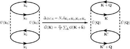
Figure 4: A second-order term in the generating functional $\Phi$ of the Hubbard model. The dashed line represents the interaction $U$, and the solid line on the left hand side (right hand side) the lattice (coarse-grained) single-particle Green function $G$ ($\bar{G}$). When the DCA Laue function is used to describe momentum conservation at the internal vertices, the wave-vectors collapse onto those of the cluster and each lattice Green function is replaced by its coarse-grained average.

The resulting compact graphs are functionals of the coarse grained Green function $\bar{G}({\bf{K}})$ and interaction ${\bar{U}}({\bf{K}})$, and thus depend on the cluster momenta ${\bf{K}}$ only. For example, when $N_{c}=1$, only the local part of the interaction survives the coarse graining. As with the CDMFT, within the DCA it is important that both the interaction and the Green function are coarse-grained Hettler et al. (2000). As a consequence of the collapse of the $\Phi$-diagrams, the DCA self-energy

$$\Sigma_{c}({\bf{K}},z)=\frac{\delta\Phi[\bar{G}({\bf{K}},z),\bar{U}]}{\delta\bar{G}({\bf{K}},z)}$$ (61)

only depends on the cluster momenta ${\bf{K}}$.

To obtain the DCA estimate of the lattice grand potential, we substitute the DCA approximate generating functional $\Phi[\bar{G}({\bf{K}}),\bar{U}({\bf{K}})]$ into Eq. (45). The grand potential is stationary with respect to ${\bf{G}}$ when

$$\frac{\delta\Omega[\bar{G}({\bf{K}}),\bar{U}({\bf{K}})]}{\delta G({\bf{k}})}=\Sigma_{c}({\bf{K}})-\Sigma({\bf{k}})=0\,,$$ (62)

which means that $\Sigma({\bf{k}})=\Sigma_{c}({\bf{K}})$ is the proper approximation for the lattice self-energy corresponding to $\Phi[\bar{G}({\bf{K}}),\bar{U}]$. The self-consistency condition on the left hand side of Eq. (44) then becomes the coarse-graining relation

$$\bar{G}({\bf{K}},z)=\frac{N_{c}}{N}\sum_{\tilde{{\bf{k}}}}[G_{0}^{-1}({\bf{K}}+{\tilde{{\bf{k}}}})-\Sigma_{c}({\bf{K}},z)]^{-1}\,.$$ (63)

with the bare Green function $G_{0}({\bf{K}}+{\tilde{{\bf{k}}}},z)=[z-\epsilon_{{\bf{K}}+{\tilde{{\bf{k}}}}}+\mu]^{-1}$.

Both the CDMFT and the DCA have well defined limits. In the infinite size cluster limit $N_{c}\to\infty$, the CDMFT and DCA approximations to the Laue function recover the exact Laue function, $\Phi$ is evaluated with the full lattice Green function and interactions and thus the exact result is recovered. When $N_{c}=1$, both the Laue functions reduce to $\Delta=1$, $\Phi$ is evaluated with the local Green function and local contributions of the interactions, and the DMFT result is recovered.

II.2.4 Self-consistency scheme

The two equations (44) form a non-linear set of equations which have to be solved self-consistently to determine the cluster self-energy ${\bf\Sigma}_{c}[\bar{\bf G}]$ with the use of a suitable cluster solver. For cluster solvers that sum up all diagrams of ${\bf\Sigma}_{c}$, i.e. in contrast to a skeletal expansion of ${\bf\Sigma}_{c}$, an additional step is necessary in the self-consistent cycle. In order to not overcount self-energy diagrams, ${\bf\Sigma}_{c}$ is to be calculated as a functional of the corresponding bare propagator to $\bar{\bf G}$, the cluster excluded Green function

$${\boldsymbol{\cal G}}(z)=[\bar{\bf G}^{-1}(z)+{\bf\Sigma}_{c}(z)]^{-1}$$ (64)

This equation unambiguously defines the self-consistent iteration procedure illustrated in Fig. 5:

1. The iteration is started by guessing an initial cluster self-energy ${\bf\Sigma}_{c}(z)$, usually zero or the result from second order perturbation theory, to

2. Calculate the coarse grained quantities

   $$\bar{\bf G}(z)=\frac{N_{c}}{N}\sum_{\tilde{{\bf{k}}}}[{\bf G}_{0}^{-1}({\tilde{{\bf{k}}}},z)-{\bf\Sigma}_{c}(z)]^{-1}\,\,,\,\bar{\bf U}=\frac{N_{c}}{N}\sum_{\tilde{{\bf{k}}}}{\bf U}({\tilde{{\bf{k}}}})$$

3. The effective cluster problem is then set up with the cluster excluded Green function $\boldsymbol{\cal G}(z)$ and $\bar{\bf U}$.

4. The self-energy ${\bf\Sigma}_{c}(z)$ or respectively the cluster Green function ${\bf G}_{c}(z)$ is calculated in the effective cluster model (see Sec. II.4) by using any of the quantum cluster solvers discussed in Sec. III.

5. For techniques that produce the cluster Green function ${\bf G}_{c}$ rather than the self-energy, the new estimate of the cluster self-energy is calculated as ${\bf\Sigma}_{c}(z)=\boldsymbol{\cal G}^{-1}(z)-{{\bf G}_{c}}^{-1}(z)$.

The iteration closes by re-calculating the coarse-grained Green function $\bar{\bf G}(z)$ in step (2) with the new estimate of the cluster self-energy. This procedure is repeated until the cluster Green function ${\bf G}_{c}(z)$ equals the coarse-grained Green function $\bar{\bf G}(z)$ to within the desired accuracy.

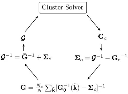
Figure 5: Sketch of the CDMFT and DCA embedded cluster algorithms. The iteration starts with computing the coarse grained Green function $\bar{\bf G}$ using an initial guess for the cluster self-energy ${\bf\Sigma}_{c}.$ The cluster excluded Green function $\boldsymbol{\cal G}$ is then used to define the effective cluster problem which yields a new estimate of ${\bf\Sigma}_{c}$.

II.3 Discussion

In contrast to the DMFT, a unique setup for the embedded cluster theory does not exist. Depending on the treatment of e.g. boundary conditions (see Sec. II.1 and Biroli and Kotliar, 2002) differences in the coupling of the cluster to its environment arise (see comparison in Sec. II.3.4 below). In fact, there exist infinitely many realizations of embedded cluster theories for any given model Hamiltonian Biroli and Kotliar (2002); Okamoto et al. (2003); Potthoff et al. (2003); Potthoff (2003b), two of which we focus on in this review.

The fundamental approximation common to all approaches is that they try to go beyond conventional mean-field approximations and introduce non-local physics by replacing the unsolvable lattice Hamiltonian by some manageable finite portion – possibly with effective model parameters – and reintroduce the thermodynamic limit by a mean-field type treatment of the remaining system. Thus, the influence of truly long-ranged correlations, i.e. those beyond the cluster size, is still not incorporated, but short-ranged correlations and in particular the local dynamics with respect to the cluster can ideally be treated exactly. That this can already lead to substantial renormalizations has been demonstrated in Sec. I.2 and is also well-known from the DMFT. The combination of short- to medium-ranged correlations with mean-field treatment of long-ranged physics enables the investigation of a system’s tendency to certain types of order not accessible by conventional mean-field theory. One can thus more clearly identify the possible existence of long-ranged correlations which are normally hard to establish in conventional finite-system calculations. On the other hand, it is this mean-field likeness that practically disables a proof for the appearance of a phase transition in the real model, even though the behavior of transition temperatures etc. with cluster size can give valuable hints about the system (see Sec. I.2).

II.3.1 Conservation and thermodynamic consistency

Both the DCA and CDMFT approximations are self-consistent and are $\Phi$-derivable since they satisfy Eq. (44). Thus, they are thermodynamically consistent in the Baym-Kadanoff sense. Observables calculated from the lattice Green function ${\bf G}$ agree with those calculated as derivatives of the lattice grand potential $\Omega$. Since the CPT is not self-consistent, it is not thermodynamically consistent. However, none of these approaches is conserving in the Baym-Kadanoff sense since they all violate momentum conservation. Thus, each of these approaches is likely to violate some set of the Ward identities Hettler et al. (2000).

II.3.2 Causality

One problem in any formation of an embedded cluster theory is the manifestation of causality, i.e. a physical Green function cannot have poles anywhere except on the real axis. In particular, for the fundamental quantity of the theory, the single particle Green function, this means that the proper self-energy in momentum space has to obey $\Im m\Sigma({\bf{k}},\omega+i0^{+})<0$. Early attempts to formulate cluster extensions to DMFT Schiller and Ingersent (1995) ran into exactly this problem, which e.g. manifests itself in negative single-particle spectral functions. Explicit proofs for causality can be given for the DCA Hettler et al. (2000) and the CDMFT (Kotliar et al., 2001; see also Biroli et al., 2003). More precisely, any embedded cluster theory consistent with the locator expansion (or a suitably defined cavity construction) obeys, due to Eqs. (28) and (32), causality. A closer look at Eqs. (28) and (32) also reveals how problems can arise. It is, for example, tempting to replace the well defined cluster quantity ${\bf\Sigma}_{c}(z)$ in (28) by some approximation to ${\bf\Sigma}(z)$, i.e. the full self-energy. As has been discussed in some detail by Okamoto et al. (2003) (see also Sec. II.8.2), such a procedure will in general introduce ringing phenomena and lead to acausal behavior. How strongly such a violation of causality will eventually influence the interesting low-energy results is quite likely a question of the model parameters under investigation. In any case, it must be taken as serious reason to at least doubt the quantitative accuracy of such results.

II.3.3 Reducible and irreducible quantities

Fundamental quantities like the one-particle self-energy ${\bf\Sigma}(z)$, or its many-particle counterparts entering e.g. susceptibilities, carry the whole fragile information about the many-body physics of a given model. In the language of diagrammatic perturbation theory they are built of so-called irreducible diagrams. Hence they are also frequently called irreducible quantities; in contrast, the single-particle Green function or a susceptibility is a reducible quantity. It is an important aspect, that the cluster theories discussed use approximants for these irreducible quantities only, i.e. the quantities obtained as derivatives of the Baym-Kadanoff $\Phi$ functional. In fact, in the formulation in Sec. II.2 any attempt to replace reducible quantities like the one-particle Green function directly by approximants is at least dangerous.

To see this, consider the grand potential functional Eq. (45). It is expressed as a sum over all closed connected distinct graphs constructed from the Green function ${\bf G}$ and interaction ${\bf U}$. The subset of compact graphs comprise the Baym-Kadanoff generating functional $\Phi[{\bf G},{\bf U}]$ which is expressed as a skeletal graph sum over all distinct compact closed connected graphs. Compact diagrams have no internal parts representing corrections to the Green function ${\bf G}$.

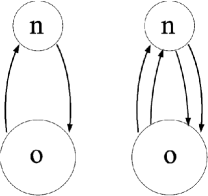
Figure 6: Non-compact (left) and compact (right) non-local corrections to the grand potential. Here the upper (lower) circle is meant to represent a set of graphs which are closed except for the external lines shown, and restricted to site $n$ (the origin).

In quantum cluster theories the graphs for $\Phi$ are approximated by their cluster counterparts. As an example, consider the limit of infinite dimensions, used by Metzner and Vollhardt to derive the DMFT Metzner and Vollhardt (1989). In this limit most closed connected graphs are local since the Green function falls off quickly with distance $r$, $G(r)\sim D^{-r/2}$. In fact, only a small set of graphs, corresponding to non-compact corrections, remain finite. To see this, consider the simplest non-local corrections to non-compact and compact parts of the grand potential of a Hubbard-like model, illustrated in Fig. 6. Here the upper (lower) circle is a set of graphs composed of intra-site propagators restricted to site $n$ (the origin). Consider all such non-local corrections on the shell of sites which are $n$ mutually orthogonal unit translations from the origin. In the limit of high dimensions, there are $2^{n}D!/((D-n)!n!)\sim{\cal{O}}(D^{n})$ such sites. Since as $D\to\infty$, $G(r)\sim D^{-r/2}$Metzner and Vollhardt (1989), the legs on the compact correction contribute a factor ${\cal{O}}(D^{-2n})$ whereas those on the non-compact correction contribute ${\cal{O}}(D^{-n})$. Therefore the compact non-local correction falls as $D^{-n}$ and vanishes as $D\to\infty$; whereas, the non-compact correction remains of order one, regardless of how far site $n$ is from the origin. As a result, the generating functional, which is composed of only compact graphs, is a functional of the local Green function and interaction in this limit

$$\Phi[{\bf G},{\bf U}]=\Phi[G_{ii},U_{ii}]+{\cal{O}}(1/D)\,.$$ (65)

A similar analysis was done for the DCA cluster problem by Aryanpour et al. (2002). They find that the corrections from sites outside the cluster associated with compact diagrams are quite small (i.e. high order in the linear cluster size $1/L_{c}$) justifying the approximation

$$\Phi[{\bf G},{\bf U}]\approx\Phi[\bar{G}({\bf{K}}),\bar{U}({\bf{K}})]\,,$$ (66)

while those associated with non-compact diagrams are large and cannot be neglected. The same analysis may be done for the CDMFT, simply by replacing the DCA graphs by those for the CDMFT.

Thus, the essential approximation for the DMFT, the DCA and the CDMFT is to approximate the lattice generating functional $\Phi$ by its cluster counterpart in the estimate of the lattice grand potential, Eq. (45). Concommittantly the derivatives of $\Phi$, i.e. the lattice self-energy and vertex functions are approximated by their respective cluster counterparts. This once more underlines why in embedded cluster theories it is necessary to always work with the cluster irreducible quantities; they are the only quantities compatible with the cluster and any attempt to include more information by e.g. Fourier transformation will lead to consistency problems, which eventually express themselves as causality violation. Irreducible quantities are also those important to discuss the convergence behavior of a cluster method with increasing cluster size as discussed in the next section.

II.3.4 Comparison

Detailed comparisons of the DCA and CDMFT algorithms were presented in Maier and Jarrell (2002), Maier et al. (2002b), Biroli and Kotliar (2002) and Biroli et al. (2003). Both approximations share the underlying idea and general algorithm, and differ only in the form used for the hopping matrix ${\bf t}$ (see Eq. (35)). The purpose of this section is to convey the consequences of this, at first sight, small difference on the effective cluster problem, convergence properties and the calculation of the lattice self-energy.

Nature of effective cluster problem.

For notational convenience, we use a 1D model with nearest neighbor hopping $t$ only, set the on-site energy $\epsilon_{o}=0$ and denote the cluster size by $L_{c}$. The generalization to higher dimension or longer-ranged hopping terms is straightforward.

The CDMFT uses the original form for the hopping matrix ${\bf t}({\tilde{k}})$ which is obtained e.g. as an inter-cluster Fourier transform (see Eq. (22)) of ${\bf t}({\tilde{x}})$.Only entries between neighboring sites inside the cluster $[{\bf t}({\tilde{k}})]_{X_{i},X_{i}\pm 1}=-t$ and between neighboring sites on the surface of the cluster $[{\bf t}({\tilde{k}})]_{X_{i},X_{i}\pm(L_{c}-1)}=-te^{\mp i{\tilde{k}}L_{c}}$ are finite. The former entries form the intra-cluster hopping matrix ${\bf t}_{c}=N_{c}/N\sum_{\tilde{k}}{\bf t}({\tilde{k}})$ while the latter entries form the inter-cluster hopping matrix $\delta{\bf t}({\tilde{k}})={\bf t}({\tilde{k}})-{\bf t}_{c}$. Both amplitudes are given by the original hopping $t$. For the effective cluster problem this translates to the fact that only sites on the surface of the cluster couple to the effective medium, while sites inside the cluster only couple to their neighboring sites in the cluster. Hence the cluster problem has open boundary conditions and translational invariance is violated within the cluster. The lattice Green function ${\bf G}({\tilde{k}})$ (see Eq. (30)) is a matrix in the cluster sites and cannot be diagonalized by going over to cluster $K$-space. Therefore the coarse-graining step Eq. (31) is done in real space.

The DCA restores translational invariance by setting $[{\bf t}_{DCA}({\tilde{k}})]_{X_{i}X_{j}}=[{\bf t}({\tilde{k}})]_{X_{i}X_{j}}e^{-i{\tilde{k}}\cdot(X_{i}-X_{j})}$ (see Eq. (35)). As a consequence, its matrix elements become identical and are given by $-te^{\mp i{\tilde{k}}}$ between sites $X_{j}=X_{i}\mp 1$ and $X_{j}=X_{i}\pm(L_{c}-1)$. Hence the DCA hopping matrix ${\bf t}_{DCA}({\tilde{k}})$ is fully cyclic with respect to the cluster sites and the lattice Green function ${\bf G}({\tilde{k}})$ is diagonalized by going over to cluster $K$-space. The DCA intra-cluster hopping matrix ${\bf t}_{c,DCA}=N_{c}/N\sum_{\tilde{k}}{\bf t}_{DCA}({\tilde{k}})$ is also cyclic with finite matrix-elements

$$[{\bf t}_{c,DCA}]_{X_{i},X_{j}}=-t\frac{L_{c}}{\pi}\sin\frac{\pi}{L_{c}}$$ (67)

between sites $X_{j}=X_{i}\pm 1$ and $X_{j}=X_{i}\pm(L_{c}-1)$ and the DCA cluster problem therefore has periodic boundary conditions. At finite cluster size $L_{c}$, the intra-cluster hopping is reduced by the factor $1/6(\pi/L_{c})^{2}+{\cal O}((\pi/L_{c})^{4})$ compared to its lattice counterpart $t$. In the infinite cluster size limit it becomes $t$. This reduction in the intra-cluster coupling is compensated by the inter-cluster hopping which is of long-ranged nature,

$$[\delta{\bf t}_{DCA}({\tilde{x}})]_{X_{i}X_{j}}=-t[\frac{\sin[({\tilde{x}}\mp 1)\pi/L_{c}]}{({\tilde{x}}\mp 1)\pi/L_{c}}-\frac{\sin(\pi/L_{c})}{\pi/L_{c}}\delta_{{\tilde{x}},0}]$$ (68)

between sites $X_{j}=X_{i}\mp 1$ and $X_{j}=X_{i}\pm(L_{c}-1)$. It is important to note that $\delta{\bf t}_{DCA}$ couples all the sites in the cluster to sites in the effective medium. It vanishes for ${\tilde{x}}=0$ and decreases as $1/{\tilde{x}}$ with increasing ${\tilde{x}}$. We also notice that

$$\delta{\bf t}_{DCA}\sim 1/L_{c}$$ (69)

for large linear cluster sizes $L_{c}$ and emphasize that this result holds generally in any dimension $D$.

The restoration of translational invariance in the DCA is achieved by mapping the lattice onto a cluster with periodic boundary conditions with reduced hopping integrals $t_{c,DCA}$ and coupling every site in the cluster to a neighboring site in the effective medium through long-ranged hopping integrals $\delta t_{DCA}({\tilde{x}})$. The sum of all finite intra- and inter-cluster couplings for a given site is again given by the original value $t$. Similar conclusions about the nature of the effective CDMFT and DCA cluster problems were reached in a study of the large $U$ limit of the Falicov-Kimball model (FKM, see Eq. (186)), i.e. the classical Ising model Biroli et al. (2003).

We stress that clusters with linear size $L_{c}=2$ are special. Here both terms in the intra-cluster hopping Eq. (67) give a contribution to the same matrix-element. Hence the nearest-neighbor hopping is given by $-2t\left(L_{c}/\pi\right)\sin\left(\pi/L_{c}\right)$, i.e. with the prefactor $-2t$ instead of $-t$ for larger clusters. This reflects the fact that every site sees its nearest neighbor twice due to the periodic boundary conditions. Non-local fluctuations are thus enhanced in clusters with linear size $L_{c}=2$ as seen e.g. in an over-proportional suppression of transition temperatures (see Secs. IV.2 and IV.4.2).

Convergence with cluster size.

The differences in boundary conditions translate directly to different asymptotic behaviors for large cluster sizes $N_{c}$. In leading order the hybridization with the mean-field, ${\bf\Gamma}$ vanishes like $\delta{\bf t}^{2}$ as the cluster size increases (see Eqs. (33) and (43)). In the CDMFT the magnitude of $\delta{\bf t}$ is of order one for the sites on the surface of the cluster and zero otherwise. The average hybridization per cluster site in the CDMFT thus scales like

$$\bar{\Gamma}_{CDMFT}=\frac{1}{N_{c}}{\rm Tr}\,[{\bf\Gamma}_{CDMFT}]\sim{\cal O}(\frac{1}{L_{c}})\,,$$ (70)

where the trace runs over cluster sites and frequency. This behavior is evident since only the $2D(L_{c}^{D-1})$ sites on the surface contribute to the sum and $N_{c}=L_{c}^{D}$. In the DCA, $\delta{\bf t}={\cal O}(1/L_{c})$ (see Eq. (69)). The average hybridization of the DCA cluster to the effective medium hence scales faster to zero as

$$\bar{\Gamma}_{DCA}=\frac{1}{N_{c}}{\rm Tr}\,[{\bf\Gamma}_{DCA}]\sim{\cal O}(\frac{1}{L_{c}^{2}})$$ (71)

since each of the $N_{c}$ terms contributes a term of the order ${\cal O}(1/L_{c}^{2})$.

It can further be shown that ${\bf\Gamma}$ acts as the small parameter in these theories: The approximation performed by the DCA and the CDMFT is to replace the lattice Green function $G$ by its coarse-grained quantity $\bar{G}$ in diagrams for the generating functional $\Phi$ (see Sec. II.2). Both Green functions differ by the inter-cluster hopping $\delta{\bf t}({\tilde{{\bf{k}}}})$, the self-energy and the hybridization function ${\bf\Gamma}$. Since the diagrams in $\Phi$ are summed over ${\tilde{{\bf{k}}}}$, the terms having the same order as $\delta{\bf t}({\tilde{{\bf{k}}}})$ vanish since $N_{c}/N\sum_{\tilde{{\bf{k}}}}\delta{\bf t}({\tilde{{\bf{k}}}})=0$. If we assume that the self-energy has corrections of the same or higher order in $1/L_{c}$ as ${\bf\Gamma}$, the convergence of $\Phi$ is entirely determined by ${\bf\Gamma}$. With the scaling relations (70) and (71) we find for the CDMFT that $\Phi_{CDMFT}\approx\Phi+{\cal O}(1/L_{c})$ while the DCA converges like $\Phi_{DCA}\approx\Phi+{\cal O}(1/L_{c}^{2})$. Since ${\bf\Sigma}=\delta\Phi/\delta{\bf G}$, it converges with $L_{c}$ as the corresponding $\Phi$ confirming the assumption. The generating functional $\Phi$ and hence the grand potential thus converges faster in the DCA than in the CDMFT with increasing cluster size.

Numerical comparison.

The scaling behavior Eqs. (70) and (71) of the CDMFT and DCA average hybridization strengths was verified numerically in the 1D FKM in Maier and Jarrell (2002) (see also Maier et al., 2002b). Here we review the effects of the different scaling behaviors of the average hybridization on the phase transition in this model. The Hamiltonian of the FKM is discussed in Sec. IV.2, Eq. (186). It can be considered as a simplified Hubbard model with only one spin-species being allowed to hop. However it still shows a complex phase diagram including a Mott gap for large $U$ at half filling, an Ising-like charge ordering with the corresponding transition temperature $T_{c}$ being zero in 1D, and phase separation in all dimensions. Since the 1D FKM is in the 1D Ising universality class we expect similar scaling behavior as observed in the results for the 1D Ising model in Sec. I.2. In particular, we expect finite transition temperatures within both cluster approximations due to their residual mean-field character. The CDMFT and DCA effective cluster models were solved with a QMC approach described in Hettler et al. (2000).

The DCA transition temperature $T_{c}$ was determined from the divergence of the lattice charge susceptibility $\chi(Q)$ calculated from the particle-hole correlation function as detailed in Sec. II.6. In the CDMFT formalism the calculation of lattice susceptibilities is difficult if not impossible due to the lack of translational invariance. Here $T_{c}$ is determined from the calculation of the charge order parameter $m$ as detailed in Sec. II.5. For the DCA both techniques are illustrated in the inset to Fig. 7.

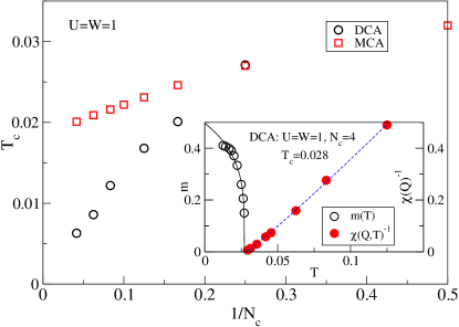
Figure 7: Transition temperature versus inverse cluster size calculated with DCA/QMC (circles) and CDMFT/QMC (squares) when $U=W=4t=1$. Inset: DCA order parameter $m(T)$ and inverse charge susceptibility $\chi(Q)^{-1}$ versus temperature. Taken from Maier et al. (2002b).

As for the 1D Ising model (see Fig. 2 in Sec. I.2), the DCA result for $T_{c}$ scales to zero almost linearly in $1/N_{c}$ for large $N_{c}$. Moreover, $T_{c}$ obtained from DCA is smaller and thus closer to the exact result than the $T_{c}$ obtained from CDMFT. The CDMFT does not show any scaling behavior and in fact seems to tend to a finite value for $T_{c}$ as $N_{c}\rightarrow\infty$. As explained above, this striking difference can be attributed to the different boundary conditions. The open boundary conditions of the CDMFT cluster result in a large surface contribution so that $\bar{\Gamma}_{CDMFT}>\bar{\Gamma}_{DCA}$. This engenders pronounced mean-field behavior that stabilizes the finite temperature transition for the cluster sizes treated in Fig. 7. For larger cluster sizes the bulk contribution to the CDMFT grand potential should dominate so that $T_{c}$ is expected to fall to zero.

Complementary results are found in simulations of finite size systems. In general, systems with open boundary conditions are expected to have a surface contribution in the grand potential of order ${\cal O}(1/L_{c})$ Fisher and Barber (1972). This term is absent in systems with periodic boundary conditions. As a result, simulations of finite size systems with periodic boundary conditions converge much more quickly than those with open boundary conditions Landau (1976).

The DCA converges faster than the CDMFT for critical properties as well as extended cluster quantities due to the different boundary conditions and the coupling to the mean-field. As detailed above, each site in the DCA cluster experiences the same coupling to the effective medium, while in the CDMFT only the sites on the boundary of the cluster couple to the mean-field host. Provided that the system is far from a transition, the sites in the center of the CDMFT cluster couple to the mean-field only through propagators which fall exponentially with distance. Local results such as the single-particle density of states thus converge more quickly in the CDMFT when measured on a central site (see Maier et al., 2002b).

Calculation of the lattice self-energy.

Another significant difference between the two cluster techniques appears in the calculation on the lattice self-energy. The DCA approximates the lattice self-energy by a constant within a DCA cell in momentum space, $\Sigma({\bf{K}}+{\tilde{{\bf{k}}}},z)=\Sigma_{c}({\bf{K}},z)$. Therefore the self-energy is a step function in ${\bf{k}}$-space. In order to obtain smooth non-local quantities such as the Fermi surface or the band structure, an interpolated $\Sigma({\bf{k}},z)$ may be used. Bilinear interpolation in 2D is guaranteed to preserve the sign of the function however leads to kinks in $\Sigma({\bf{k}},z)$. Yielding the smoothest possible interpolation of $\Sigma({\bf{K}},z)$, the use of an Akima spline which does not overshoot is consistent with the DCA assumption that the self-energy is a smoothly varying function in ${\bf{k}}$-space. However it is important to note that this interpolated self-energy should not be used in the self-consistent loop as this can lead to violations of causality as discussed above.

In the CDMFT, the lattice self-energy is given by the Fourier transform of the cluster self-energy (see Eq. (56))

$$\Sigma({\bf{k}},{\bf{k}}^{\prime},z) = \frac{1}{N_{c}}\sum_{\bf{Q}}\sum_{{\bf X}_{i},{\bf X}_{j}}e^{-i{\bf{k}}\cdot{\bf X}_{i}}\Sigma_{c}({\bf X}_{i},{\bf X}_{j},z)e^{i{\bf{k}}^{\prime}\cdot{\bf X}_{j}}$$ (72)

$$\times\,\,\delta({\bf{k}}-{\bf{k}}^{\prime}-{\bf{Q}})\,.$$

Since the CDMFT cluster violates translational invariance, the lattice self-energy depends on two momenta ${\bf{k}}$ and ${\bf{k}}^{\prime}$ which can differ by a wave-vector ${\bf{Q}}$ of the cluster reciprocal space. To restore translational invariance, the CDMFT approximates the lattice self-energy by the ${\bf{Q}}=0$ contribution to give Kotliar et al. (2001)

$$\Sigma({\bf{k}},z)=\frac{1}{N_{c}}\sum_{{\bf X}_{i},{\bf X}_{j}}e^{-i{\bf{k}}\cdot({\bf X}_{i}-{\bf X}_{j})}\Sigma_{c}({\bf X}_{i},{\bf X}_{j},z)\,.$$ (73)

In real space, the lattice self-energy

$$\Sigma({\bf x}_{i},{\bf x}_{j},z)=\frac{1}{N_{c}}\sum_{{\bf X}_{i},{\bf X}_{j}}\Sigma_{c}({\bf X}_{i},{\bf X}_{j})\delta_{{\bf X}_{i}-{\bf X}_{j},{\bf x}_{i}-{\bf x}_{j}}$$ (74)

is thus obtained by averaging over those cluster self-energy elements $\Sigma({\bf X}_{i},{\bf X}_{j})$ where the distance ${\bf X}_{i}-{\bf X}_{j}$ equals the distance ${\bf x}_{i}-{\bf x}_{j}$. As explained in Biroli and Kotliar (2002), the factor $1/N_{c}$ leads to an underestimation of non-local self-energy contributions at small cluster sizes, since the number of contributions for fixed ${\bf x}_{i}-{\bf x}_{j}>0$ in the sum Eq. (74) is always smaller than $N_{c}$. As a possible solution to this problem, Biroli and Kotliar (2002) suggested to replace the form (74) for the lattice self-energy by a weighted sum which preserves causality. One could e.g. weight the terms in the sum by their number instead of $N_{c}$ to achieve better results.

It is important to note that as in the DCA, the lattice self-energy Eq. (73) or (74) does not enter the self-consistent loop. Biroli et al. (2003) however realized that a translational invariant formulation of the CDMFT algorithm can be obtained by replacing the cluster self-energy ${\bf\Sigma}_{c}(z)$ by the translationally invariant lattice self-energy ${\bf\Sigma}({\tilde{{\bf{k}}}})$, Eq. (73) in the coarse-graining step Eq. (53). Despite the dependence on ${\tilde{{\bf{k}}}}$, this form of ${\bf\Sigma}({\tilde{{\bf{k}}}})$ can be shown to preserve causality Biroli et al. (2003).

II.4 Effective cluster model

Quantum cluster approaches reduce the complexity of the lattice problem with infinite degrees of freedom to a (numerically) solvable system with $N_{c}$ degrees of freedom. As detailed in Sec. II.2 this is achieved through the approximation of $\Phi[{\bf G},{\bf U}]$, the exact Baym-Kadanoff functional of the exact Green function ${\bf G}$ and interaction ${\bf U}$, by a spatially localized quantity $\Phi[\bar{\bf G},\bar{\bf U}]$ which is a functional by the corresponding (coarse-grained) quantities restricted to the cluster sites, $\bar{\bf G}=N_{c}/N\sum_{\tilde{{\bf{k}}}}{\bf G}({\tilde{{\bf{k}}}})$ and $\bar{\bf U}=N_{c}/N\sum_{\tilde{{\bf{k}}}}{\bf U}({\tilde{{\bf{k}}}})$.

$\Phi[\bar{\bf G},\bar{\bf U}]$ may be calculated non-perturbatively as the solution of a quantum cluster model

$${\cal H}_{c}=H_{c,0}+H_{c,I}\,.$$ (75)

${\cal H}_{c}$ consists of a non-interacting term $H_{c,0}$ describing the bare cluster degrees of freedom and their coupling to a host. The interacting term $H_{c,I}$ is related to the corresponding term in the original lattice model through the coarse-grained interaction $\bar{\bf U}$. This ensures that the functional dependencies of the cluster functional $\Phi_{c}$ and its lattice counterpart $\Phi$ are identical.

The non-interacting term $H_{c,0}$ is fixed by the requirement that the Green function ${\bf G}_{c}$ of the cluster model equals the coarse-grained Green function $\bar{\bf G}$ of the original model

$${\bf G}_{c}\equiv\bar{\bf G}=[\boldsymbol{\cal G}^{-1}-{\bf\Sigma}_{c}]^{-1}\,,$$ (76)

and hence is specified by the cluster-excluded Green function $\boldsymbol{\cal G}$ (see Eq. (64)).

For Green function or respectively action based cluster solvers, like e.g. perturbation theory or QMC, $H_{c,0}$ can hence be encoded in the cluster-excluded Green function $\boldsymbol{\cal G}$. The corresponding cluster action $S_{c}$ for the fermionic cluster degrees of freedom represented by the Grassman variables $\gamma$, $\gamma^{*}$ reads in imaginary time and cluster real space

$$S_{c}[\gamma,\gamma^{*}]=-\int\limits_{0}^{\beta}d\tau\int\limits_{0}^{\beta}d\tau^{\prime}\sum_{ij,\sigma}\gamma^{*}_{i\sigma}(\tau){\cal{G}}_{ij,\sigma}(\tau-\tau^{\prime})\gamma_{j\sigma}(\tau^{\prime})$$

$$+\int\limits_{0}^{\beta}d\tau\sum_{ij,\sigma\sigma^{\prime}}\frac{\bar{U}_{ij}}{2}\gamma^{*}_{i\sigma}(\tau)\gamma^{*}_{j\sigma^{\prime}}(\tau)\gamma_{j\sigma^{\prime}}(\tau)\gamma_{i\sigma}(\tau)\,,$$ (77)

where we used the short hand notation $i,j$ for the cluster sites ${\bf X}_{i},{\bf X}_{j}$. Note that for the CDMFT the quantities ${\cal{G}}_{ij}$ and $\bar{U}_{ij}$ are given by Eqs. (64) and (54) respectively, while for the DCA they are given by the cluster Fourier transforms of ${\cal{G}}({\bf{K}})=[\bar{G}^{-1}({\bf{K}},z)+\Sigma_{c}({\bf{K}},z)]^{-1}$ and respectively of $\bar{U}({\bf{K}})$ (see Eq. (60)).

For Hamiltonian-based techniques, like e.g. the non-crossing approximation, exact diagonalization or numerical renormalization group, the need for an explicit formulation of $H_{c,0}$ is inevitable. To setup the bare part $H_{c,0}$, it is convenient to use Eq. (32) for the CDMFT or respectively (42) for the DCA together with Eq. (76) to represent the cluster excluded Green function $\boldsymbol{\cal G}$. In the CDMFT, we have with Eq. (28)

$$\boldsymbol{\cal G}(z)=[(z+\mu)\mathbb{1}-{\bf t}_{c}-{\bf\Gamma}(z)]^{-1}\,,$$ (78)

and the matrix-elements of the intra-cluster hopping ${\bf t}_{c}$ are given by the hopping amplitudes of the original lattice, $t_{ij}$ as detailed in Sec. II.3.4. The non-interacting problem is thus split into two parts, cluster degrees of freedom with hopping integrals $t_{ij}$ and their coupling to a dynamic host described by the hybridization function ${\bf\Gamma}(z)$. The CDMFT cluster model can hence be written as (see also Bolech et al., 2003)

$${\cal H}_{c}=H_{c,0}+H_{c,I} = \sum_{ij,\sigma}(t_{ij}-\mu\delta_{ij})c^{\dagger}_{i\sigma}c_{j\sigma}$$ (79)

$$+ \sum_{ij,{\tilde{{\bf{k}}}},\sigma}\lambda_{ij{\tilde{{\bf{k}}}}}[a^{\dagger}_{i{\tilde{{\bf{k}}}}\sigma}a_{j{\tilde{{\bf{k}}}}\sigma}+h.c.]$$

$$+ \sum_{ij,{\tilde{{\bf{k}}}},\sigma}[V_{ij}({\tilde{{\bf{k}}}})c_{i\sigma}^{\dagger}a_{j{\tilde{{\bf{k}}}}\sigma}+h.c.]$$

$$+ \sum_{ij,\sigma\sigma^{\prime}}\frac{\bar{U}_{ij}}{2}c^{\dagger}_{i\sigma}c^{\dagger}_{j\sigma^{\prime}}c_{j\sigma^{\prime}}c_{i\sigma}\,.$$

The first part describes the isolated cluster degrees of freedom with fermionic creation (destruction) operators $c^{\dagger}_{i\sigma}$ ($c_{i\sigma}$). The second term simulates the host degrees of freedom as a non-interacting conduction band with the help of auxiliary operators $a^{\dagger}_{i{\tilde{{\bf{k}}}}\sigma}$ ($a_{i{\tilde{{\bf{k}}}}\sigma}$) and energy levels $\lambda_{ij{\tilde{{\bf{k}}}}}$. The coupling between the cluster states and the bath with an amplitude $V_{ij}({\tilde{{\bf{k}}}})$ is described by the third term and the interacting term is given by the last term. The sums over ${\tilde{{\bf{k}}}}$ run over the $N/N_{c}$ wave-vectors of the superlattice. Integrating out the auxiliary degrees of freedom yields an action of the form (II.4) with

$${\cal{G}}_{ij}(z) = [(z+\mu)\mathbb{1}-{\bf t}_{c}-{\bf\Gamma}_{c}(z)]_{ij}^{-1}$$ (80)

$$\Gamma_{c,ij}(z) = \sum_{lm,{\tilde{{\bf{k}}}}}V_{il}^{*}({\tilde{{\bf{k}}}})[z\mathbb{1}-{\bf\lambda}({\tilde{{\bf{k}}}})]^{-1}_{lm}V_{mj}({\tilde{{\bf{k}}}})\,.$$ (81)

Self-consistency then requires that the auxiliary parameters $\lambda_{ij{\bf{k}}}$ and $V_{ij}({\tilde{{\bf{k}}}})$ are chosen in a way such that the cluster hybridization function ${\bf\Gamma}_{c}(z)$ is identical to its lattice counterpart ${\bf\Gamma}(z)$ defined in Eq. (78). It is important to note that, while the isolated cluster parameter ${\bf t}_{c}$ can be deduced directly from the non-interacting part of the lattice system, the energy levels $\lambda_{\bf{k}}$ and coupling constants $V_{ij}({\bf{k}})$ of the auxiliary particles are not known a-priori, but determined by the self-consistency condition ${\bf\Gamma}_{c}={\bf\Gamma}$. Since $\Gamma_{ij}$ is only finite on the surface of the cluster (see discussion in Sec. II.3.4), the coupling $V_{ij}({\tilde{{\bf{k}}}})$ between the cluster and the host is only finite for sites $i$ on the surface of the cluster which effectively reduces the number of baths. This was numerically verified in CDMFT exact diagonalization studies by Bolech et al. (2003).

For the DCA we have with Eqs. (41) and (42)

$${\cal{G}}({\bf{K}},z)=[z-\bar{\epsilon}_{\bf{K}}+\mu-\Gamma({\bf{K}},z)]^{-1}\,,$$ (82)

and hence the DCA effective cluster model is best represented in cluster ${\bf{K}}$-space as

$${\cal H}_{c} = H_{c,0}+H_{c,I}$$ (83)

$$= \sum_{{\bf{K}},\sigma}(\bar{\epsilon}_{\bf{K}}-\mu)c^{\dagger}_{{\bf{K}}\sigma}c_{{\bf{K}}\sigma}+\sum_{{\bf{k}},\sigma}\lambda_{\bf{k}}a^{\dagger}_{{\bf{k}}\sigma}a_{{\bf{k}}\sigma}$$

$$+ \sum_{{\bf{K}},{\tilde{{\bf{k}}}},\sigma}[V_{{\bf{K}}}({\tilde{{\bf{k}}}})c_{{\bf{K}}\sigma}^{\dagger}a_{{\bf{K}}+{\tilde{{\bf{k}}}}\sigma}+h.c.]$$

$$+ \sum_{\stackrel{{\scriptstyle{\bf{K}},{\bf{K}}^{\prime}}}{{{\bf{Q}}}}}\sum_{\sigma\sigma^{\prime}}\frac{\bar{U}({\bf{Q}})}{2N_{c}}c^{\dagger}_{{\bf{K}}+{\bf{Q}}\sigma}c^{\dagger}_{{\bf{K}}^{\prime}-{\bf{Q}}\sigma^{\prime}}c_{{\bf{K}}^{\prime}\sigma^{\prime}}c_{{\bf{K}}\sigma}\,.$$

The operators $c^{\dagger}_{{\bf{K}}\sigma}$ ($c_{{\bf{K}}\sigma}$) create (destroy) an electron with momentum ${\bf{K}}$ and spin $\sigma$ on the cluster. $\bar{U}({\bf{Q}})$ is the Coulomb repulsion between electrons on the cluster defined in Eq. (60) and the sum over ${\tilde{{\bf{k}}}}$ in the coupling term again is restricted to the $N/N_{c}$ wave-vectors of the superlattice. Analogous to the CDMFT case it is easy to see that the DCA cluster model yields an action of the form (II.4) (in cluster Fourier space) with a ${\cal{G}}$ of the form (82) and the cluster hybridization function

$$\Gamma_{c}({\bf{K}},z)=\frac{N_{c}}{N}\sum_{{\tilde{{\bf{k}}}}}\frac{|V_{\bf{K}}({\tilde{{\bf{k}}}})|^{2}}{z-\lambda_{{\bf{K}}+{\tilde{{\bf{k}}}}}}\,.$$ (84)

The auxiliary parameters of the DCA cluster model are then determined by the condition $\Gamma_{c}({\bf{K}})=\Gamma({\bf{K}})$.

For $N_{c}=1$ both the CDMFT and the DCA cluster models reduce to the single-impurity Anderson model. If self-consistency is also established on the two-particle level (see discussion at the end of Sec. II.1) via a susceptibility, an additional coupling to a bosonic field representing the corresponding fluctuations has to be considered in the cluster model (for details see Maier, 2003). For $N_{c}=1$ the cluster model then reduces to the effective impurity model used in the EDMFT approach Smith and Si (2000).

As detailed in Sec. II.1, the CPT formalism sets the hybridization function ${\bf\Gamma}$ to zero, i.e considers an isolated cluster without the coupling to a host. Thus the CPT cluster model is identical to the original lattice model restricted to cluster sites, i.e. given by the first and last terms of the CDMFT cluster model Eq. (79).

II.5 Phases with broken symmetry

For simplicity, in the preceding sections the self-consistent equations of quantum cluster theories have been derived assuming the absence of symmetry-breaking. In Sec. II.6 we review how instabilities to ordered phases can be identified by the computation of response functions. However, to explore the nature as well as possible coexistence of symmetry-broken states, generalizations of the cluster algorithms that explicitly account for the possibility of symmetry-breaking on the single-particle level are necessary.

The applicability and modifications required to treat symmetry broken phases depend on the cluster approach. The CPT formalism is not amenable to the description of ordered phases because its self-energy is that of a finite isolated cluster in which spontaneous symmetry breaking cannot occur. However, Dahnken et al. developed a variational extension of the CPT Dahnken et al. (2003) based on the self-energy functional approach by Potthoff (2003b) which yields a self-consistent scheme to study ordered phases (for details see Sec. II.8). The CDMFT formalism can describe ordered phases which are identifiable by a broken translational symmetry (such as antiferromagnetism) by construction, since the translational symmetry of the CDMFT cluster is already broken (see Maier and Jarrell, 2002; Maier et al., 2002b; Biroli et al., 2003). Hence translational invariant solutions are often found to be unstable against the ordered one Biroli et al. (2003). The DCA formalism is translationally invariant by construction, and therefore generalizations of the algorithm are necessary to treat ordered phases. To keep this section concise, we exemplify the necessary generalizations of the DCA formalism to a selection of relevant types of symmetry-broken phases along with the mapping onto the corresponding cluster models. The adoption of the presented concepts to the CDMFT approach is straightforward.

Once the equations are generalized to account for symmetry breaking, the requisite algorithmic changes are relatively simple. A finite conjugate external field is used to initialize the calculation and break the symmetry. The field is then switched off after a few iterations and the system relaxes to its equilibrium state in the absence of external fields. On the other hand, if the field remains small and finite, the dependence of the order parameter on the field can be determined and used as an alternate way to calculate the susceptibility (by extrapolation to zero field). This approach is especially useful for cluster solvers such as the non-crossing approximation or the fluctuation-exchange approximation where the computation of two-particle correlation functions is numerically too expensive.

II.5.1 Uniform magnetic field – Ferromagnetism

We first consider the formalism necessary to treat ferromagnetism. A finite homogeneous external magnetic field $h$ is introduced which acts on the spin $\sigma$ of the fermions according to the Zeeman term

$$-h\sum_{i,\sigma}\sigma c^{\dagger}_{i\sigma}c_{i\sigma}\,.$$ (85)

The effect of $h$ on the motion of the spatial degree of freedom of the electrons, i.e. the diamagnetic term, is neglected for simplicity.

In the presence of finite $h$ or a uniform magnetization, the single-particle Green functions for up- and down-electrons are not equivalent. To account for this $SU(2)$ symmetry-breaking, the spin-index of the Green function $G_{\sigma}$, self-energy $\Sigma_{\sigma}$ and effective medium ${\cal{G}}_{\sigma}$ (and hence $\Gamma_{\sigma}$) in the derivation of the DCA-equations has to be retained. For a finite uniform magnetic field $h$ the DCA lattice Green function reads

$$G_{\sigma}({\bf{k}},z)=\frac{1}{z-\epsilon_{{\bf{K}}+{\tilde{{\bf{k}}}}}+\mu+h\sigma-\Sigma_{c,\sigma}({\bf{K}},z)}\,$$ (86)

and the coarse grained and corresponding cluster-excluded Green function

$$\bar{G}_{\sigma}({\bf{K}},z) = \frac{N_{c}}{N}\sum_{\tilde{{\bf{k}}}}G_{\sigma}({\bf{K}}+{\tilde{{\bf{k}}}},z)\,,$$ (87)

$${\cal{G}}^{-1}_{\sigma}({\bf{K}},z) = G^{-1}_{\sigma}({\bf{K}},z)+\Sigma_{c,\sigma}({\bf{K}},z)$$ (88)

become spin-dependent.

The action of the effective cluster model is identical to the action in the paramagnetic state, Eq. (II.4), but the spin indices have to be explicitly retained. It then describes electrons in an external magnetic field $h$ coupled to a spin-dependent host and self-consistency is established by equating the Green function of the cluster model with the coarse-grained Green function (87).

In analogy, for Hamiltonian based cluster solvers, an additional term

$$-h\sum_{{\bf{K}},\sigma}\sigma c^{\dagger}_{{\bf{K}}\sigma}c_{{\bf{K}}\sigma}$$ (89)

is added to the cluster Hamiltonian, Eq. (83), in the presence of a finite external magnetic field $h$. The coarse-grained Green function $\bar{G}$, Eq. (86), is then used to calculate the magnetization $m:=1/N\sum_{i\sigma}\sigma\langle n_{i\sigma}\rangle$ according to

$$m=\frac{1}{N_{c}}\sum_{{\bf{K}},\sigma}\sigma\bar{G}_{\sigma}({\bf{K}},\tau=0^{-})$$ (90)

and after analytical continuation

$$m=-\frac{1}{\pi}\frac{1}{N_{c}}\sum_{{\bf{K}}\sigma}\sigma\int\limits_{-\infty}^{+\infty}d\omega f(\omega)\Im m\bar{G}_{\sigma}({\bf{K}},\omega+i\delta)\,.$$ (91)

II.5.2 Superconductivity

In this and the next section we generalize the DCA formalism to treat phases with superconducting and antiferromagnetic order, respectively. For better readability, we refrain from discussing the description of phases with coexisting superconducting and antiferromagnetic order. The extension to an integrated formalism is straightforward and has been discussed in Lichtenstein and Katsnelson (2000).

We consider superconducting phases where the electrons are paired in spin singlet or triplet states with $S_{z}=0$ indicated by finite values of the order parameter $\Delta_{\bf{k}}:=\langle c_{{\bf{k}}\uparrow}c_{-{\bf{k}}\downarrow}\rangle$ for some ${\bf{k}}$. In addition to the normal Green function $G({\bf{k}},\tau)$ it is therefore necessary to introduce the anomalous Green function $F({\bf{k}},\tau)=-\langle T_{\tau}c_{{\bf{k}}\uparrow}(\tau)c_{-{\bf{k}}\downarrow}\rangle$. The spatial and temporal symmetry of the pairing state can then be inferred from the symmetries of $F$. Since $F$ describes the pairing of fermions, it necessarily is antisymmetric under the exchange of two particles. The spatial symmetry of the pairing state is determined by the ${\bf{k}}$-dependence of the anomalous Green function $F({\bf{k}},\tau)$. If we assume conventional even-frequency pairing $F({\bf{k}},-\tau)=F({\bf{k}},\tau)$, in the case of spin-singlet pairing, $F$ has to be symmetric in ${\bf{k}}$, i.e. $F(-{\bf{k}},\tau)=F({\bf{k}},\tau)$ as is the case for even parity order parameters such as e.g. $s$-wave and $d$-wave. In the case of spin-triplet pairing $F$ is antisymmetric in ${\bf{k}}$. i.e. $F(-{\bf{k}},\tau)=-F({\bf{k}},\tau)$ as e.g. in a $p$-wave state.

The allowed symmetry of the pairing state is restricted by the cluster geometry. It depends upon the ${\bf{k}}$-dependence of the dispersion $\epsilon_{\bf{k}}$ and the ${\bf{K}}$-dependence of the cluster self-energy ${\bf\Sigma}({\bf{K}},\tau)$. When $N_{c}=1$, ${\bf\Sigma}$ is local and the ${\bf{k}}$-dependence of $F({\bf{k}},\tau)$ is entirely through $\epsilon_{\bf{k}}$. Hence only pairing states with the symmetry of the lattice such as $s$-wave and extended $s$-wave can be described by this formalism Jarrell (1992); Jarrell and Pruschke (1993). Larger cluster sizes are necessary to describe order-parameters with a symmetry less than the lattice symmetry, e.g. simulations with $N_{c}=4$ are necessary to describe phases with a $d_{x^{2}-y^{2}}$-wave order parameter which transforms according to $\cos k_{x}-\cos k_{y}$.

By utilizing the concept of Nambu-spinors

$$\Psi^{\dagger}_{\bf{k}}:=(c^{\dagger}_{{\bf{k}}\uparrow},c_{-{\bf{k}}\downarrow})\,;\,\Psi_{\bf{k}}=(\Psi^{\dagger}_{\bf{k}})^{\dagger}$$ (92)

the self-consistent equations can be written in a more compact form, since the corresponding Green function matrix in Nambu space

$${\bf G}({\bf{k}},z):=\langle\langle\Psi_{\bf{k}};\Psi^{\dagger}_{\bf{k}}\rangle\rangle_{z}=\left(\begin{array}[]{cc}G({\bf{k}},z)&F({\bf{k}},z)\\ F^{*}({\bf{k}},z^{*})&-G^{*}(-{\bf{k}},-z^{*})\end{array}\right)$$ (93)

contains information about both the normal and anomalous Green functions. In the presence of an external pairing field $\eta({\bf{k}})=\eta^{\prime}({\bf{k}})+i\eta^{\prime\prime}({\bf{k}})$ which couples to $c_{-{\bf{k}}\downarrow}c_{{\bf{k}}\uparrow}$, the non-interacting part of the Hubbard Hamiltonian can be written as $H_{0}=\sum_{{\bf{k}}}\Psi^{\dagger}_{\bf{k}}[\epsilon_{\bf{k}}\sigma_{3}-\eta^{\prime}({\bf{k}})\sigma_{1}+\eta^{\prime\prime}({\bf{k}})\sigma_{2}]\Psi_{\bf{k}}$ so the the DCA lattice Green function in the superconducting state becomes

$${\bf G}({\bf{k}},z) = [z\sigma_{o}-(\epsilon_{{\bf{k}}}-\mu)\sigma_{3}$$ (94)

$$-\eta^{\prime}({\bf{k}})\sigma_{1}-\eta^{\prime\prime}({\bf{k}})\sigma_{2}-{\bf\Sigma}_{c}({\bf{K}},z)]^{-1}\,,$$

where ${\bf{k}}={\bf{K}}+{\tilde{{\bf{k}}}}$ and $\sigma_{i}$ are the Pauli-spin matrices. The diagonal parts of the Nambu-matrix ${\bf\Sigma}_{c}({\bf{K}},z)$ describe quasiparticle renormalizations and the off-diagonal parts contain information about the ${\bf{K}}$- and frequency dependence of the pairing state. Again, the coarse-grained Green function

$$\bar{\bf G}({\bf{K}},z) = \frac{N_{c}}{N}\sum_{\tilde{{\bf{k}}}}{\bf G}({\bf{K}}+{\bf{k}},z)$$ (97)

$$= \left(\begin{array}[]{cc}\bar{G}({\bf{K}},z)&\bar{F}({\bf{K}},z)\\ \bar{F}^{*}({\bf{K}},z^{*})&-\bar{G}^{*}(-{\bf{K}},-z^{*})\end{array}\right)$$

is used to calculate the cluster-excluded Green function

$$\boldsymbol{\cal G}({\bf{K}},z)=[\bar{\bf G}^{-1}({\bf{K}},z)+{\bf\Sigma}_{c}({\bf{K}},z)]^{-1}$$ (98)

which together with the coarse-grained interaction $\bar{U}({\bf{K}})$ defines the action of the corresponding effective cluster model

$$S_{c}=-\int\limits_{0}^{\beta}d\tau\int\limits_{0}^{\beta}d\tau^{\prime}\sum_{ij}{\boldsymbol{\psi}}_{i}^{\dagger}(\tau)\boldsymbol{\cal G}_{ij}(\tau-\tau^{\prime}){\boldsymbol{\psi}}_{j}(\tau^{\prime})$$

$$+\int\limits_{0}^{\beta}d\tau\sum_{ij}\frac{\bar{U}_{ij}}{2}\left[{\boldsymbol{\psi}}_{i}^{\dagger}(\tau)\sigma_{3}{\boldsymbol{\psi}}_{i}(\tau)\right]\left[({\boldsymbol{\psi}}_{j}^{\dagger}(\tau)\sigma_{3}{\boldsymbol{\psi}}_{j}(\tau)\right]\,.$$ (99)

As in the normal state case (see Eq. (II.4)), the cluster action is represented in cluster real space and all the quantities are cluster Fourier transforms of the corresponding quantities in cluster ${\bf{K}}$-space. The spinors of Grassmann-variables ${\boldsymbol{\psi}}_{i}^{\dagger}=(\gamma_{i\uparrow}^{*},\gamma_{i\downarrow})$ and ${\boldsymbol{\psi}}_{i}=({\boldsymbol{\psi}}_{i}^{\dagger})^{\dagger}$ generate coherent states corresponding to the cluster Fourier transform of the Nambu-spinors Eq. (92). In analogy, the corresponding cluster Hamiltonian in the superconducting state is obtained from the normal state cluster Hamiltonian Eq. (83) by representing it with the Nambu-spinors (92) and adding a U(1) symmetry breaking term

$$-\sum_{{\bf{K}}}\Psi^{\dagger}_{\bf{K}}[\bar{\eta}^{\prime}({\bf{K}})\sigma_{1}-\bar{\eta}^{\prime\prime}({\bf{K}})\sigma_{2}]\Psi_{\bf{K}}\,,$$ (100)

where $\bar{\eta}({\bf{K}})=N_{c}/N\sum_{\tilde{{\bf{k}}}}\eta({\bf{K}}+{\tilde{{\bf{k}}}})$ is the coarse-grained pair-field.

After self-consistency is established by requiring that the Green function of the effective cluster model calculated with the action Eq. (II.5.2) equals the coarse-grained Green function Eq. (97), the order parameter $\Delta_{\bf{k}}$ can be calculated. Within the DCA the resolution in ${\bf{k}}$-space is restricted to the cluster ${\bf{K}}$-points and the order parameter is coarse-grained

$$\bar{\Delta}_{\bf{K}}=\frac{N_{c}}{N}\sum_{\tilde{{\bf{k}}}}\langle c_{{\bf{K}}+{\tilde{{\bf{k}}}}\uparrow}c_{-({\bf{K}}+{\tilde{{\bf{k}}}})\downarrow}\rangle=\bar{F}({\bf{K}},\tau=0^{+})$$ (101)

and given by the equal-time coarse-grained anomalous Green function $\bar{F}$ as (after analytical continuation)

$$\bar{F}({\bf{K}},\tau=0^{+})=\frac{1}{\beta}\sum_{n}\bar{F}({\bf{K}},i\omega_{n})$$

$$=\frac{1}{\pi}\int\limits_{0}^{\infty}d\omega\tanh\left(\frac{\beta\omega}{2}\right)\Im m\bar{F}({\bf{K}},\omega+i\delta)\,.$$ (102)

II.5.3 Antiferromagnetic order

In this section we derive the DCA cluster formalism for antiferromagnetism on a bipartite lattice. This formalism is appropriate when $N_{c}>1$. A formalism suitable for the case when $N_{c}=1$ is discussed in detail in Georges et al. (1996) in the context of DMFT.

The antiferromagnetically ordered state is characterized by a spatial variation of the magnetization according to

$${\bf m}({\bf x})={\bf m}e^{i{\bf{Q}}\cdot{\bf x}}\,,$$ (103)

where ${\bf x}$ denotes the sites in the lattice and ${\bf{Q}}$ is the antiferromagnetic wave-vector (${\bf{Q}}=(\pi,\pi)$ in 2D). Hence bipartite lattices can be divided into two inequivalent sublattices according to

$$e^{i{\bf{Q}}\cdot{\bf x}}=\left\{\begin{array}[]{rcl}1&:&{\bf x}\in\mbox{A sub-lattice}\\ -1&:&{\bf x}\in\mbox{B sub-lattice}\end{array}\right.\,.$$ (104)

The magnetic ordering thus reduces the translational symmetry of the original lattice. The volume of the magnetic unit cell is doubled compared to the structural unit cell. Accordingly, the volume of the first Brillouin zone in the antiferromagnetic state is reduced to half the original volume and ${\bf{Q}}=(\pi,\pi)$ becomes a reciprocal lattice vector. Hence in neutron scattering experiments Bragg peaks are found at the wave-vector ${\bf{Q}}$ corresponding to a period of two lattice spacings.

As a consequence of the translational symmetry breaking, the correlation function

$$G_{\sigma}({\bf{k}},{\bf{k}}+{\bf{Q}};\tau)=-\langle T_{\tau}c_{{\bf{k}}\sigma}(\tau)c^{\dagger}_{{\bf{k}}+{\bf{Q}}\sigma}\rangle$$ (105)

becomes finite. Along the lines of the formalism for the superconducting state it is thus convenient to introduce spinors

$$\Psi^{\dagger}_{{\bf{k}}\sigma}=(c^{\dagger}_{{\bf{k}}\sigma},c^{\dagger}_{{\bf{k}}+{\bf{Q}}\sigma})\,;\,\,\Psi_{{\bf{k}}\sigma}=(\Psi_{{\bf{k}}\sigma}^{\dagger})^{\dagger}$$ (106)

for the antiferromagnetic state. In the presence of a staggered external magnetic field $h({\bf x})=h\exp(i{\bf{Q}}\cdot{\bf x})$ the non-interacting part of the Hamiltonian for bipartite lattices with $\epsilon_{{\bf{k}}+{\bf{Q}}}=-\epsilon_{\bf{k}}$ then becomes $H_{0}=\sum_{{\bf{k}}\sigma}^{\prime}\Psi^{\dagger}_{{\bf{k}}\sigma}(\epsilon_{\bf{k}}\sigma_{3}-\sigma\frac{h}{2}\sigma_{1})\Psi_{{\bf{k}}\sigma}$ where the prime on the sum indicates summation over the reduced Brillouin zone only. The corresponding Green function

$${\bf G}_{\sigma}({\bf{k}},z) = \langle\langle\Psi_{{\bf{k}}\sigma};\Psi^{\dagger}_{{\bf{k}}\sigma}\rangle\rangle_{z}$$

$$= [z\sigma_{o}-(\epsilon_{\bf{k}}-\mu)\sigma_{3}-\sigma\frac{h}{2}\sigma_{1}-{\bf\Sigma}_{c}({\bf{K}},z)]^{-1}\,,$$

with ${\bf{k}}={\bf{K}}+{\tilde{{\bf{k}}}}$, is coarse-grained over the DCA cells

$$\bar{\bf G}_{\sigma}({\bf{K}}) = \frac{N_{c}}{N}\sum_{\tilde{{\bf{k}}}}{\bf G}_{\sigma}({\bf{K}}+{\tilde{{\bf{k}}}})$$ (108)

$$= \left(\begin{array}[]{cc}\bar{G}_{\sigma}({\bf{K}},{\bf{K}})&\bar{G}_{\sigma}({\bf{K}},{\bf{K}}+{\bf{Q}})\\ \bar{G}_{\sigma}({\bf{K}}+{\bf{Q}},{\bf{K}})&\bar{G}_{\sigma}({\bf{K}}+{\bf{Q}},{\bf{K}}+{\bf{Q}})\end{array}\right)\,,$$ (111)

where we dropped the frequency argument for convenience. The cluster excluded Green function

$$\boldsymbol{\cal G}_{\sigma}({\bf{K}},z) = [\bar{\bf G}^{-1}_{\sigma}({\bf{K}},z)+{\bf\Sigma}_{c,\sigma}({\bf{K}},z)]^{-1}\,.$$ (112)

then has two elements, ${\cal{G}}_{\sigma}({\bf{K}},{\bf{K}})$ and ${\cal{G}}_{\sigma}({\bf{K}},{\bf{K}}+{\bf{Q}})$. As a result, its Fourier transform to real space

$${\cal{G}}_{ij,\sigma} = \frac{1}{N_{c}}\sum_{\bf{K}}e^{i{\bf{K}}\cdot({\bf X}_{i}-{\bf X}_{j})}{\cal{G}}_{\sigma}({\bf{K}})$$

$$+ \frac{1}{N_{c}}\sum_{\bf{K}}e^{i{\bf{K}}\cdot({\bf X}_{i}-{\bf X}_{j})}e^{-i{\bf{Q}}\cdot{\bf x}_{j}}{\cal{G}}_{\sigma}({\bf{K}},{\bf{K}}+{\bf{Q}})$$

breaks translational symmetry. The action of the corresponding cluster model in the antiferromagnetic state is then formally identical to the action in the paramagnetic state, Eq. (II.4). As in the superconducting state the corresponding cluster model is obtained from the paramagnetic cluster model Eq. (83) by changing the representation to the Nambu spinors Eq. (106) and adding a symmetry breaking term

$$-\sum_{{\bf{K}}\sigma}\sigma\frac{h}{2}\Psi^{\dagger}_{{\bf{K}}\sigma}\sigma_{1}\Psi_{{\bf{K}}\sigma}\,,$$ (114)

to account for the external staggered magnetic field $h$.

After convergence, the sub-lattice magnetization $m=1/N\sum_{i\sigma}e^{i{\bf{Q}}\cdot{\bf x}_{i}}\sigma\langle n_{i\sigma}\rangle$ may be calculated from the off-diagonal component of the Green function matrix Eq. (108) according to

$$m = \frac{1}{N_{c}}\sum_{{\bf{K}}\sigma}\sigma\bar{G}_{\sigma}({\bf{K}},{\bf{K}}+{\bf{Q}};\tau=0^{-})$$

$$= -\frac{1}{N_{c}\pi}\sum_{{\bf{K}}\sigma}\int\limits_{-\infty}^{+\infty}d\omega f(\omega)\sigma\Im m\bar{G}_{\sigma}({\bf{K}},{\bf{K}}+{\bf{Q}};\omega+i\delta)\,.$$

II.6 Calculation of susceptibilities

A convenient way to identify continuous phase transitions is to search for divergences of susceptibilities. One particular advantage of quantum cluster theories is that they allow us to consistently calculate these susceptibilities from the corresponding cluster susceptibilityHettler et al. (2000). Unfortunately, the calculation of two-particle correlation functions in the CDMFT formalism is strongly hampered by the violation of translational invariance on the cluster. So, in this section, we will restrict our attention to the calculation of two-particle quantities in th DCA following Hettler et al. (2000) and Jarrell et al. (2001b).

As a specific example, we describe here the calculation of the two-particle Green function

$$\chi_{\sigma\sigma^{\prime}}(q,k,k^{\prime}) = \int_{0}^{\beta}\int_{0}^{\beta}\int_{0}^{\beta}\int_{0}^{\beta}d\tau_{1}d\tau_{2}d\tau_{3}d\tau_{4}$$

$$\times e^{i\left((\omega_{n}+\nu)\tau_{1}-\omega_{n}\tau_{2}+\omega_{n^{\prime}}\tau_{3}-(\omega_{n^{\prime}}+\nu)\tau_{4}\right)}$$

$$\times \langle T_{\tau}c_{{\bf{k}}+{\bf{q}}\sigma}^{{\dagger}}(\tau_{1})c_{{\bf{k}}\sigma}(\tau_{2})c_{{\bf{k}}^{\prime}\sigma^{\prime}}^{{\dagger}}(\tau_{3})c_{{\bf{k}}^{\prime}+{\bf{q}}\sigma^{\prime}}(\tau_{4})\rangle\,,$$

where we adopt the conventional notation Abrikosov et al. (1963) $k=({\bf{k}},i\omega_{n})$, $k^{\prime}=({\bf{k}},i\omega_{n^{\prime}})$, $q=({\bf{q}},i\nu_{n})$ and $T_{\tau}$ is the time ordering operator.

$\chi_{\sigma\sigma^{\prime}}(q,k,k^{\prime})$ and the irreducible two-particle vertex function $\Gamma_{\sigma\sigma^{\prime}}(q,k,k^{\prime})$ (not to be confused with the single-particle hybridization function) are related to each other through the Bethe-Salpeter equation

$$\chi_{\sigma\sigma^{\prime}}(q,k,k^{\prime})=\chi^{0}_{\sigma\sigma^{\prime}}(q,k,k^{\prime})+\chi^{0}_{\sigma\sigma^{\prime\prime}}(q,k,k^{\prime\prime})$$

$$\times\,\,\Gamma_{\sigma^{\prime\prime}\sigma^{\prime\prime\prime}}(q,k^{\prime\prime},k^{\prime\prime\prime})\chi_{\sigma^{\prime\prime\prime}\sigma^{\prime}}(q,k^{\prime\prime\prime},k^{\prime})$$ (116)

where $\chi^{0}_{\sigma\sigma^{\prime}}(q,k,k^{\prime\prime})$ is the non-interacting susceptibility constructed from a pair of fully-dressed single-particle Green functions. As usual, a summation is to be made for repeated indices.

We now make the DCA substitution $\Gamma_{\sigma\sigma^{\prime}}({\bf{q}},{\bf{K}}+{\tilde{{\bf{k}}}},{\bf{K}}^{\prime}+{\tilde{{\bf{k}}}}^{\prime})\to{\Gamma_{c}}_{\sigma\sigma^{\prime}}\left({\bf{q}},{\bf{K}},{\bf{K}}^{\prime}\right)$ in Eq. (II.6) where $\Gamma_{c}$ is the irreducible two-particle vertex calculated on the cluster (frequency labels have been suppressed). Note that only the bare and dressed two-particle Green functions $\chi$ depend upon the superlattice wave-vectors ${\tilde{{\bf{k}}}}$. Since $\chi$ and $\chi^{0}$ in the product on the RHS of Eq. (II.6) share no common momentum labels, we may freely sum over the wave-vectors ${\tilde{{\bf{k}}}}$, yielding

$$\bar{\chi}_{\sigma\sigma^{\prime}}(q,K,K^{\prime})=\bar{\chi}^{0}_{\sigma\sigma^{\prime}}(q,K,K^{\prime})+\bar{\chi}^{0}_{\sigma\sigma^{\prime\prime}}(q,K,K^{\prime\prime})$$ (117)

$$\times {\Gamma_{c}}_{\sigma^{\prime\prime}\sigma^{\prime\prime\prime}}(q,K^{\prime\prime},K^{\prime\prime\prime})\bar{\chi}_{\sigma^{\prime\prime\prime}\sigma^{\prime}}(q,K^{\prime\prime\prime},K^{\prime})\,.$$

By coarse-graining the Bethe-Salpeter equation, we have greatly reduced its complexity; each of the matrices above is sufficiently small that they may be easily manipulated using standard techniques.

In contrast with the single-particle case where the coarse-grained quantities are identical to those of the cluster, the cluster quantity ${\chi_{c}}_{\sigma\sigma^{\prime}}(q,K,K^{\prime})$ is not equal to $\bar{\chi}_{\sigma\sigma^{\prime}}(q,K,K^{\prime})$. This is because the self-consistency is established only at the single-particle level. Unlike the single-particle case where both $\Sigma_{c}(K)$ and ${\bar{G}}(K)$ are directly calculated, neither ${\Gamma_{c}}_{\sigma\sigma^{\prime}}(q,K,K^{\prime})$ nor the coarse-grained susceptibility $\bar{\chi}_{\sigma\sigma^{\prime}}(q,K,K^{\prime})$ are calculated during the self-consistency. Instead, the coarse-grained non-interacting susceptibility $\bar{\chi}^{0}_{\sigma\sigma^{\prime}}(q,K,K^{\prime})$ is calculated in a separate program after the DCA converges using the relation

$$\bar{\chi}^{0}_{\sigma\sigma^{\prime}}[({\bf{q}},i\nu_{n});({\bf{K}},i\omega_{n});({\bf{K}}^{\prime},i\omega_{n^{\prime}})]=\delta_{\sigma\sigma^{\prime}}\delta_{{\bf{K}}{\bf{K}}^{\prime}}\delta_{\omega_{n}\omega_{n^{\prime}}}$$

$$\times\frac{N_{c}}{N}\sum_{{\tilde{k}}}G_{\sigma}({\bf{K}}+{\bf{\tilde{k}}},i\omega_{n})G_{\sigma}({{\bf{K}}+{\bf{\tilde{k}}}+{\bf{q}}},i\omega_{n}+\nu_{n})\quad\mbox{.}$$ (118)

The corresponding cluster susceptibility is calculated by the cluster solver, e.g. the QMC process, as discussed in Sec. III.3.1 and the vertex function is extracted by inverting the cluster two-particle Bethe-Salpeter equation

$${\chi_{c}}_{\sigma\sigma^{\prime}}(q,K,K^{\prime})={\chi_{c}}^{0}_{\sigma\sigma^{\prime}}(q,K,K^{\prime})+{\chi_{c}}^{0}_{\sigma\sigma^{\prime\prime}}(q,K,K^{\prime\prime})$$

$$\times{\Gamma_{c}}_{\sigma^{\prime\prime}\sigma^{\prime\prime\prime}}(q,K^{\prime\prime},K^{\prime\prime\prime}){\chi_{c}}_{\sigma^{\prime\prime\prime}\sigma^{\prime}}(q,K^{\prime\prime\prime},K^{\prime})\,.$$ (119)

If we combine Eqs. (II.6) and (117), then the coarse-grained susceptibility may be obtained after elimination of ${\Gamma_{c}}_{\sigma\sigma^{\prime}}(q,K,K^{\prime})$ between the two equations. It reads

$${\bar{\boldsymbol{\chi}}}^{-1}={\boldsymbol{\chi}}_{c}^{-1}-{\boldsymbol{\chi}}_{c}^{0^{-1}}+{\bar{\boldsymbol{\chi}}}^{0^{-1}}\,,$$

where, for example, ${\bar{\boldsymbol{\chi}}}$ is the matrix formed from $\bar{\chi}_{\sigma,\sigma^{\prime}}(q,K,K^{\prime})$ for fixed $q$. The charge $(ch)$ and spin $(sp)$ susceptibilities ${\chi}_{ch,sp}(q,T)$ are deduced from $\bar{\chi}$ according to

$${\chi}_{ch,sp}(q,T)=\frac{(k_{B}T)^{2}}{N_{c}^{2}}\sum_{KK^{\prime}\sigma\sigma^{\prime}}\lambda_{\sigma\sigma^{\prime}}\bar{\chi}_{\sigma\sigma^{\prime}}(q,K,K^{\prime})\,,$$ (120)

where $\lambda_{\sigma\sigma^{\prime}}=1$ for the charge channel and $\lambda_{\sigma\sigma^{\prime}}=\sigma\sigma^{\prime}$ for the spin channel. The calculation of particle-particle (i.e. pairing) susceptibilities follows from a straightforward generalization of this formalism. The reader is referred to prior articles on cluster QMC for more details on these topics Jarrell et al. (2001b).

II.7 Disordered systems

In this section, we describe cluster approximations for disordered systems. The mapping between the lattice and the cluster in the CDMFT and the molecular CPA (MCPA) is identical, and when the CDMFT is applied to disordered systems, it becomes identical to the MCPA Tsukada (1969); Ducastelle (1974). The MCPA and related techniques for disordered systems are extensively reviewed in Gonis (1992) and will not be discussed here.

In the remainder of this section we describe a DCA for disordered systems that recovers the CPA for $N_{c}=1$ and becomes exact when $N_{c}\to\infty$. This is an extension of the formalism introduced by Jarrell and Krishnamurthy (2001), modified to include the effects of correlated disorder Jarrell and Johnson (2004). We consider an Anderson model with diagonal disorder, described by the Hamiltonian

$$H=\displaystyle-t\sum_{<ij>,\sigma}\left(c^{\dagger}_{i\sigma}c_{j\sigma}+c^{\dagger}_{j\sigma}c_{i\sigma}\right)\\ \displaystyle+\sum_{i\sigma}(V_{i}-\mu)n_{i\sigma}$$ (121)

where $c^{\dagger}_{i\sigma}$ creates a quasiparticle on site $i$ with spin $\sigma$ and $n_{i\sigma}=c^{\dagger}_{i\sigma}c_{i\sigma}$. The disorder occurs in the site occupancies labeled by $\xi_{i}$ and in the local orbital energies $V_{i}$ which describe the electrostatic potential at site $i$. We assume that $V_{i}$ are quenched random variables distributed according to some specified probability distribution which includes the effects of intersite correlations.

The effect of the disorder potential $\sum_{i\sigma}V_{i}n_{i,\sigma}$ may be described using standard diagrammatic perturbation theory (although we eventually sum to all orders). We perturb around the ordered state, described by the first term in Eq. (121).

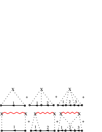
Figure 8: A few low-order diagrams in the irreducible self-energy of a quenched diagonally disordered system. Each circle represents the scattering of a state ${\bf{k}}$ from sites denoted by X and a dotted line. The correlations between the electrostatic potentials on different sites are denoted by the wavy line.

Translational invariance and momentum conservation are restored by averaging over all allowed values of the site occupancies $\{\xi_{i}\}$ and the corresponding disorder potentials $V_{i}$. We study this effect, e.g., on the sixth graph shown in Fig. 8 which makes a contribution to the self-energy

$$\frac{1}{N^{4}}\sum_{i\neq j,{\bf{k}}_{1},{\bf{k}}_{2},{\bf{k}}_{3}}\langle V_{i}^{2}V_{j}^{2}\rangle G({\bf{k}}_{1})G({\bf{k}}_{2})G({\bf{k}}_{3})$$

$$\hskip 28.45274pt\times\,\,e^{i{\bf x}_{i}\cdot({\bf{k}}_{1}-{\bf{k}}+{\bf{k}}_{3}-{\bf{k}}_{2})}e^{i{\bf x}_{j}\cdot({\bf{k}}_{2}-{\bf{k}}_{1}+{\bf{k}}^{\prime}-{\bf{k}}_{3})}$$ (122)

After averaging over the disorder configurations, $\langle V_{i}^{2}V_{j}^{2}\rangle$ becomes a function of ${\bf x}_{i}-{\bf x}_{j}$. We identify this average as $D_{ij}^{22}$. With translational invariance restored, we may complete the Fourier transform, and obtain

$$\frac{\delta_{{\bf{k}}{\bf{k}}^{\prime}}}{N^{3}}\sum_{{\bf{k}}_{1},{\bf{k}}_{2},{\bf{k}}_{3},{\bf{q}}}D^{22}({\bf{q}})G({\bf{k}}_{1})G({\bf{k}}_{2})G({\bf{k}}_{3})$$

$$\left(N\delta_{{\bf{q}}+{\bf{k}}_{2}+{\bf{k}},{\bf{k}}_{1}+{\bf{k}}_{3}}-1\right)\,.$$ (123)

It is easy to extend this argument to all orders in perturbation theory. All graphs are composed of sums of products of Laue functions (e.g. $\Delta=N\delta_{{\bf{q}}+{\bf{k}}_{2}+{\bf{k}},{\bf{k}}_{1}+{\bf{k}}_{3}}$), and Green functions $G({\bf{k}})$ and $D^{nm}({\bf{q}})$, where $D^{nm}({\bf{q}})$ is the Fourier transform of $D_{ij}^{nm}=\langle V_{i}^{n}V_{j}^{m}\rangle$.

A hierarchy of approximations may then be constructed by approximating the Laue functions within the graphs. These include the CPA where conservation of the internal momentum labels is completely neglected. Here, all of the Laue functions involving the internal momentum labels are set to one, $\Delta=N\delta_{{\bf{k}}_{1}+{\bf{k}}_{2}\cdots}\to 1$. In this case we may freely sum over all internal momentum labels, and all terms describing non-local correlations, such as those on the bottom of Fig. 8 vanish, whereas the CPA graphs shown on top remain. Different cluster approximations, including the MCPA and the DCA may be constructed by systematically restoring momentum conservation through the appropriate choice of Laue function, as discussed in Sec. II.2

For the DCA, we divide the lattice into clusters as described in Fig. 3, write wave-vectors as ${\bf{k}}={\bf{K}}+{\tilde{{\bf{k}}}}$ and employ the DCA Laue function Eq. (58),

$$\Delta_{DCA}=N_{c}\delta_{{\bf{K}}_{1}+{\bf{K}}_{2},{\bf{K}}_{3}+{\bf{K}}_{4}...}\,,$$ (124)

such that momentum conservation is preserved only within the cluster reciprocal space ${\bf{K}}$. With this choice for the Laue function, we may freely sum over superlattice wave-vectors ${\tilde{{\bf{k}}}}$ within each DCA coarse-graining cell (see Fig. 3). This leads to the replacement of the lattice propagators $G({\bf{k}})$ and $D^{nm}({\bf{k}})$ with coarse-grained propagators $\bar{G}({\bf{K}})$ and ${\bar{D}}^{nm}({\bf{K}})$, respectively,

$$\bar{G}({\bf{K}},z)=\frac{N_{c}}{N}\sum_{{\tilde{{\bf{k}}}}}G({\bf{K}}+{\tilde{{\bf{k}}}},z),$$ (125)

$$\bar{D}^{nm}({\bf{K}})=\frac{N_{c}}{N}\sum_{{\tilde{{\bf{k}}}}}D^{nm}({\bf{K}}+{\tilde{{\bf{k}}}}),$$ (126)

The first of these sums is straightforward; however, the second requires some investigation due to the powers of the potential.

Here, we calculate $\bar{D}^{nm}({\bf{K}})$ for a binary $A$,$B$ alloy where the concentration of $A$ atoms is $c$ and that of $B$ atoms is $1-c$. This calculation can be generalized to multicomponent alloys and may easily be extended for more complex alloys. For the binary alloy, we employ an idempotent formalism where the idempotent $\xi_{i}=1$ indicating that the site is occupied by an $A$ atom, or $\xi_{i}=0$ indicating a $B$ atom site. If we associate $V_{i}=V_{A}$ or $V_{B}$ for an $A$ or $B$ atom, respectively, then $V_{i}=\xi_{i}V_{A}+(1-\xi_{i})V_{B}$. Then, since $\xi_{i}^{n}=\xi_{i}$ and $(1-\xi_{i})^{n}=1-\xi_{i}$,

$$\langle V_{i}^{n}V_{j}^{m}\rangle = \langle(\xi_{i}V_{A}+(1-\xi_{i})V_{B})^{n}(\xi_{j}V_{A}+(1-\xi_{j})V_{B})^{m}\rangle$$ (127)

$$= \langle(\xi_{i}V_{A}^{n}+(1-\xi_{i})V_{B}^{n})(\xi_{j}V_{A}^{m}+(1-\xi_{j})V_{B}^{m})\rangle$$

$$= V_{\alpha}^{n}V_{\beta}^{m}g_{ij}^{\beta\gamma}$$

where repeated indices in the last line are summed over and

$$g_{ij}^{AA} = \langle\xi_{i}\xi_{j}\rangle$$ (128)

$$g_{ij}^{AB} = \langle\xi_{i}(1-\xi_{j})\rangle$$ (129)

$$g_{ij}^{BB} = \langle(1-\xi_{i})(1-\xi_{j})\rangle$$ (130)

are the joint probabilities for occupation of sites $i$ and $j$ by atoms of the designated types.

This formalism may be generalized to a multicomponent alloy $\alpha=A,B,C,\dots$. Since a site may only be occupied by an atom of one type only, in general

$$\langle V_{i}^{n}V_{j}^{m}\rangle=V_{\alpha}^{n}V_{\beta}^{m}g_{ij}^{\beta\gamma}\,.$$ (131)

$\langle V_{i}^{n}V_{j}^{m}\rangle$ is a linear function of the probabilities $g_{ij}^{\beta\gamma}$ for all $n$ and $m$. Thus, the effect of coarse-graining $D^{nm}({\bf{k}})$ is equivalent to coarse-graining $g^{\beta\gamma}({\bf{k}})$ for all $n$ and $m$.

As an example, consider a binary alloy with only near-neighbor configurational correlations. Here we may write

$$g_{ij}^{\beta\gamma}=g^{0,\beta\gamma}+\alpha\left(2\delta_{\beta\gamma}-1\right)\delta_{i+\epsilon,j}$$ (132)

where $\epsilon$ indexes the near-neighbors to site $i$, and $g^{0,AA}=c^{2}$, $g^{0,BB}=(1-c)^{2}$ and $g^{0,AB}=c(1-c)$ are the joint probabilities for the occupation of different sites for a system without configurational correlations. On a hypercubic lattice of dimension $D$

$$g^{\beta\gamma}({\bf{k}})=g^{0,\beta\gamma}\delta_{{\bf{k}},0}+\alpha\left(2\delta_{\beta\gamma}-1\right)\sum_{l=1}^{D}\cos(k_{l})\,.$$ (133)

The corresponding coarse-grained result is

$$\bar{g}^{\beta\gamma}({\bf{K}})=g^{0,\beta\gamma}\delta_{{\bf{K}},0}+\alpha\left(2\delta_{\beta\gamma}-1\right)R\sum_{l=1}^{D}\cos(K_{l})$$ (134)

where $R=(L_{c}/\pi)\sin(\pi/L_{c})$ is a coarse-graining factor ($L_{c}=N_{c}^{1/D}$ is the linear cluster size). If we transform back to the cluster coordinates, then

$$\bar{g}_{ij}^{\beta\gamma}=g^{0,\beta\gamma}+R\alpha\left(2\delta_{\beta\gamma}-1\right)\delta_{i+\epsilon,j}$$ (135)

are the configurational probabilities for the cluster, where $\epsilon$ labels the sites adjacent to $i$. In the CPA limit, $L_{c}=1$ and thus $R$ vanishes indicating the lack of any configurational correlations. In the limit as $N_{c}=L_{c}^{D}\to\infty$, $R=1$, so correlations are systematically restored.

The cluster problem generated by the substitution $\Delta\to\Delta_{DCA}$ may be solved numerically. Each of the diagrams in Fig. 8 representing $N_{c}$ independent scatters, or less, remain finite; however, scattering diagrams for greater than $N_{c}$ scatters vanish. The complexity of the problem is further reduced since the nontrivial sums involve only the cluster momenta ${\bf{K}}$ ( numbering $N_{c}$ instead of $N$). Furthermore, since these diagrams are the same as those from a finite-sized periodic cluster of $N_{c}$ sites, we can easily sum this series to all orders by numerically solving the corresponding cluster problem. The resulting algorithm is identical to that presented in Sec. II.2.4, except that: 1. In the coarse-graining step we must calculate both the coarse-grained correlation function

$${\bar{g}^{\beta\gamma}}({\bf{K}})=\frac{N_{c}}{N}\sum_{\tilde{{\bf{k}}}}g^{\beta\gamma}({\bf{K}}+{\tilde{{\bf{k}}}}).$$ (136)

and the coarse-grained cluster Green function

$${\bar{G}}({\bf{K}},z)=\frac{N_{c}}{N}\sum_{\tilde{{\bf{k}}}}\frac{1}{z+\mu-\epsilon_{{\bf{K}}+{\tilde{{\bf{k}}}}}-\Sigma_{c}({\bf{K}},z)}$$ (137)

2. We then solve the cluster problem by performing a weighted average of the cluster Green function (in matrix notation in the cluster sites)

$${\bf{G}}=\left<\left(\boldsymbol{\cal G}^{-1}-{\bf{V}}\right)^{-1}\right>$$ (138)

over all disorder configurations. The weighting of each configuration is determined by the Fourier transform of ${\bar{g}^{\beta\gamma}}({\bf{K}})$ to obtain the cluster configurational probabilities ${\bar{g}^{\beta\gamma}_{ij}}$. After convergence is reached, the irreducible cluster quantities may be used to calculate the properties of the lattice.

II.8 Alternative cluster methods

In this review we decided to focus on the three, in our view most established cluster methods. This section reviews several other ideas proposed to introduce non-local correlations, some of which are complementary to the approaches discussed.

II.8.1 Self-energy functional theory

The self-energy-functional approach developed by Potthoff (2003b) (see also Potthoff et al., 2003) is a very general unifying concept for existing cluster approaches and in addition provides the power to construct novel cluster algorithms. Similar to the formalism presented in Sec. II.2, this approach views the grand potential $\Omega$ as the central quantity. Here, the self-energy ${\bf\Sigma}$ is considered the basic dynamic variable and a self-energy functional $\Omega[{\bf\Sigma}]={\rm Tr}\,ln(-({\bf G}_{0}^{-1}-{\bf\Sigma})^{-1})+F[{\bf\Sigma}]$ is constructed from the Legendre-transform $F[{\bf\Sigma}]=\Phi[{\bf G}[{\bf\Sigma}]]-{\rm Tr}({\bf\Sigma}{\bf G}[{\bf\Sigma}])$ of the $\Phi[{\bf G}]$ functional. This approach proceeds with setting up a general variational scheme to use dynamical information from a (numerically) solvable reference system $H^{\prime}=H_{0}({\bf t}^{\prime})+H_{1}({\bf U})$ to approximate the physics of the original system $H=H_{0}({\bf t})+H_{1}({\bf U})$. While the single-particle parts $H_{0}$ are generally different, the interaction part $H_{1}({\bf U})$ is kept fixed, to ensure that the functionals $F[{\bf\Sigma}]$ of the reference system and the original system share the same functional dependence. It can then be shown that the grand potential of the original system $\Omega_{\bf t}[{\bf\Sigma}]$ can be evaluated exactly according to

$$\Omega_{\bf t}[{\bf\Sigma}({\bf t}^{\prime})]=\Omega^{\prime} + {\rm Tr\,ln}(-({\bf G}_{0}^{-1}-{\bf\Sigma}({\bf t}^{\prime}))^{-1})$$ (139)

$$- {\rm Tr\,ln}(-{\bf G}^{\prime})$$

from the grand potential $\Omega^{\prime}$, the trial self-energy ${\bf\Sigma}({\bf t}^{\prime})$ and Green function ${\bf G}^{\prime}$ of the reference system. Variation is then performed with respect to the single-particle parameters ${\bf t}^{\prime}$ of the reference system and the stationary point is determined by $\partial\Omega_{\bf t}[{\bf\Sigma}({\bf t}^{\prime})]/\partial{\bf t}^{\prime}=0$.

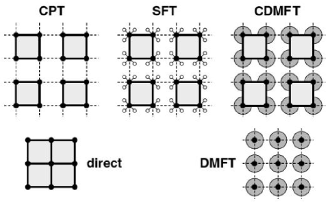
Figure 9: Taken from Potthoff et al. (2003). Various reference systems $H^{\prime}$ for the 2D Hubbard model on a square lattice. The solid and dashed lines represent the intra- and inter-cluster hopping respectively, the filled circles the on-site interaction $U$. Additional $n_{b}$ bath sites are depicted by open circles, while the shaded circles represent $n_{b}=\infty$ bath sites.

The choice of a suitable and solvable reference system $H^{\prime}$ given the original Hamiltonian $H$ is in principle arbitrary. Within the SFT, cluster approximations are constructed from a reference system $H^{\prime}$ that represents decoupled clusters of size $N_{c}$ which are optionally coupled to additional $n_{b}$ uncorrelated bath sites. A schematic illustration for the Hubbard model is shown in Fig. 9. A set of decoupled sites as a reference system $H^{\prime}$ (not shown) yields the Hubbard-I approximation. Non-local correlations can be included by considering a system of decoupled clusters of size $N_{c}>1$. This approach is identical to the CPT when the intra-cluster parameters ${\bf t}^{\prime}$ are fixed to the original values ${\bf t}$ : The self-energy of the reference system, ${\bf\Sigma}({\bf t}^{\prime})={{\bf G}^{\prime}_{0}}^{-1}-{{\bf G}^{\prime}}^{-1}$ is calculated once and used to approximate the Green function of the original lattice model, ${\bf G}^{-1}={\bf G}_{0}^{-1}-{\bf\Sigma}({\bf t}^{\prime})$. This yields the expression (47) of the CPT, ${\bf G}^{-1}={{\bf G}^{\prime}}^{-1}-\delta{\bf t}$, since the bare Green-functions of the original and reference systems only differ by the inter-cluster hopping $\delta{\bf t}$.

Alternatively within the SFT the intra-cluster hopping ${\bf t}^{\prime}$ can be treated variationally. Calculations for the 1D Hubbard model Potthoff et al. (2003) however show that the SFT functional Eq. (139) is stationary for ${\bf t}^{\prime}$ slightly larger but very close to the original value ${\bf t}$, with the difference becoming smaller as $N_{c}$ increases. The SFT can also be used to find the correct boundary conditions of the CPT cluster. Calculations with fixed intra-cluster hopping ${\bf t}^{\prime}={\bf t}$ and additional variational hopping $t_{r}$ between the surface sites to simulate periodic boundary conditions show that the self-energy functional is only stationary at $t_{r}=0$ (open boundary conditions), not at $t_{r}=t$ (periodic boundary conditions) Potthoff et al. (2003).

One shortcoming of the CPT is its inability to describe phases with broken symmetry due to the finite size of the clusters. The SFT can be used to construct a variational CPT, an extension of the CPT to account for long-range order Dahnken et al. (2003). This is done by adding a fictitious symmetry breaking single-particle term to the reference system and subtracting it in the inter-cluster part so that it has no effect on the original lattice Hamiltonian. The magnitude of this term is then optimized in the SFT variational treatment. Calculations for the 2D Hubbard model show very good agreement with variational Monte Carlo and auxiliary field Quantum Monte Carlo results for the ground-state energy and the staggered magnetization Dahnken et al. (2003).

Embedded cluster approximations are constructed if additional $n_{b}$ uncorrelated bath sites are introduced. The DMFT is obtained by choosing as a reference system a set of decoupled sites coupled to $n_{b}=\infty$ uncorrelated bath sites. The CDMFT is identical to a system of decoupled clusters coupled to $n_{b}=\infty$ bath sites with the intra-cluster parameters being fixed at the original values ${\bf t}$ and the bath parameters being treated as variational. It can then be shown Potthoff et al. (2003) that the SFT self-energy functional is stationary at the bath parameters that fulfill the CDMFT self-consistency. A corresponding analysis of the DCA formalism within this approach is still lacking.

Intermediate approximations can be constructed by considering a finite number $0<n_{b}<\infty$ of bath sites. This approach is superior to the CPT and inferior to the CDMFT. For a reference system with $N_{c}=1$ and $n_{b}=1$ this approach can be used to study the Mott transition in the Hubbard model Potthoff (2003a) analytically and it was shown to yield the same qualitative picture as the full DMFT ($N_{c}=1$, $n_{b}=\infty$) analysis (see Georges et al., 1996).

II.8.2 Fictive impurity models

Similar to the SFT approach discussed above, this very general approach by Okamoto et al. (2003) is centered on the self-energy ${\bf\Sigma}$ as the basic dynamic variable. It is based on the idea that the cluster model is merely an algorithm to calculate coefficients in an orthogonal function expansion of the momentum dependence of the electronic self-energy

$$\Sigma_{\rm approx}({\bf{k}},z)=\sum_{i=0\dots n}\Phi_{i}({\bf{k}})\Sigma_{i}(z)\,.$$ (140)

The coefficients $\Sigma_{i}(z)$ can then be obtained from the solution of a $n+1$-site fictive impurity model involving $n+1$ mean-fields which are fixed by the requirement that the impurity model Green functions $G_{i}$ equal the corresponding integrals over the lattice Green function

$$G_{i}(z)=\sum_{\bf{k}}\Phi_{i}({\bf{k}})[G^{-1}_{o}({\bf{k}},z)-\Sigma_{\rm approx}({\bf{k}},z)]^{-1}\,.$$ (141)

To include local and nearest neighbor correlations, the momentum dependence of the self-energy may be expanded up to second order using the orthogonal functions $\Phi_{0}({\bf{k}})=1$ and $\Phi_{1}({\bf{k}})=e^{ika}$. Since in general the orthogonal functions $\Phi_{i}({\bf{k}})$ change sign over the Brillouin zone except for the local term $i=0$, causality is not guaranteed when the expansion is truncated at low order. However it is shown that simple filtering of the higher-order terms may be used to circumvent these problems Okamoto et al. (2003).

The DCA may be viewed as a specific example of this approach, where the indices $i$ correspond to the centers ${\bf{K}}$ of the DCA cells and the functions $\Phi_{\bf{K}}({\bf{k}})$ are set to 1 if ${\bf{k}}$ is contained in the cell represented by ${\bf{K}}$ and 0 otherwise (see Fig. 3). Causality problems are thus avoided by using orthogonal functions which are non-negative everywhere. The resulting approximants however have discontinuities in momentum space.

II.8.3 Non-local effects via spectral density approximation

Laad and van den Bossche (2000) proposed to include non-local $1/D$-corrections by combining DMFT with the Spectral Density Approximation (SDA) Roth (1969) and applied this approach to the FKM (see Eq. (186)) for which it becomes particularly simple. In the SDA, the moments of the spectral function are determined (via repeated evaluation of commutators with the Hamiltonian) by complicated but static correlators. For the FKM, to order $1/D$ the SDA self-energy of the $d$ electrons, $\Sigma_{0,d}({\bf{k}},z)$ can be expressed in terms of the static susceptibility of the $f$-electrons. This self-energy is purely real, but momentum dependent and is used to approximate the bath self-energy in the hybridization function

$$\Gamma(z)=\sum_{{\bf{k}}}\frac{t^{2}}{z-\epsilon_{{\bf{k}}}+\mu-\Sigma_{0,d}({\bf{k}},z)}$$ (142)

for the effective impurity problem in $D=\infty$. The impurity self energy, $\Sigma_{imp,d}(z)$ (see Brandt and Mielsch, 1989) combines with the bath self-energy $\Sigma_{0,d}({\bf{k}},z)$ to a dynamical, non-local self-energy of the form

$$\Sigma_{d}({\bf{k}},z)=\Sigma_{imp,d}(z)+\Sigma_{0,d}({\bf{k}},z)-\sum_{{\bf{k}}}\Sigma_{0,d}({\bf{k}},z)\,.$$ (143)

This finally determines the Green function of the mobile $d$- electrons of the usual form, $G_{d}({\bf{k}},z)=[z-\epsilon_{{\bf{k}}}+\mu-\Sigma_{d}({\bf{k}},z)]^{-1}$, which is used together with $\Sigma_{d}({\bf{k}},z)$ to estimate the susceptibility of the $f$-electrons (see Laad and van den Bossche, 2000 for details). $\Sigma_{0,d}({\bf{k}},z)$ can then be recalculated to close the self-consistency loop.

With this method, Laad and van den Bossche studied the DOS and the spectral function $A({\bf{k}},\omega)$ of the FKM on a 2D square lattice. Their results agree well with known results and other studies like Hettler et al. (2000). On the other hand, the FKM is a particularly gentle test bed for their method, due to its effective impurity nature (mobile electrons in a static background). For a model with true dynamics like the Hubbard model, it is unclear whether the method is even feasible (due to the additional spin-flip and pair-hopping correlators), and the limitation of a purely real bath self-energy is likely to be too restrictive.

II.8.4 Non-local corrections via projection technique

Using the projection technique Tien has developed a cluster extension of the DMFT by taking into account both local and non-local contributions to the dynamics within a relevant subspace of Liouville or operator space Minh-Tien (1998, 1999a, 1999b, 2001); Tanh-Hai and Minh-Tien (2001). The information of a given subspace is stored in static susceptibility and frequency functions while the effects of the remaining subspace are collected in a dynamic memory function. The idea of Tien’s approach is to approximate this memory function by a local quantity. Hence, non-local correlations are taken into account through static quantities (susceptibilities), while dynamical correlations are approximated by a local memory function. If the relevant subspace is spanned by operators acting on the same or nearest-neighbor sites only, these quantities can be calculated in an effective impurity model Minh-Tien (1998, 1999a) or, in an improved version, in a two-site cluster model Minh-Tien (1999b, 2001); Tanh-Hai and Minh-Tien (2001).

This approach has not been rigorously proven to be causal, however its application to the Falicov-Kimball Minh-Tien (1998, 1999b) and Hubbard model Minh-Tien (2001) shows that the spectral function is positive definite and the sum-rules of the first few moments of the spectral densities are preserved. The neglect of non-local dynamical correlations however leads to spurious behavior at low temperatures: A Kondo resonance emerges in the in 2D half-filled Hubbard model at low temperatures similar to the behavior observed in DMFT simulations but inconsistent with other cluster calculations which show a pseudogap down to the lowest temperatures (see Sec. IV.4.2). This shortcoming is due to the fact that the nearest-neighbor static correlations are proportional to the band-dispersion $\epsilon_{\bf{k}}$. At the Fermi energy, $\epsilon_{\bf{k}}=0$, hence non-local correlations vanish and a Kondo-resonance is generated due to the local nature of the dynamical correlations.

II.8.5 Two-site correlations with composite operators

A dynamical non-perturbative two-site approximation for the Hubbard model based on the composite operator method was developed by Matsumoto and Mancini (1997) and later adopted and improved by Stanescu and Phillips Stanescu and Phillips (2001); Stanescu and Phillips (2003a). By using Hubbard operators as a local basis which exactly diagonalize the interaction part of the Hamiltonian, this approach recovers both the weak coupling $U\ll t$ and strong coupling $U\gg t$ limits of the Hubbard model. The memory function $\delta m({\bf{k}},\omega)$ which collects the effects of dynamical correlations is expanded in a two-site approximation as $\delta m({\bf{k}},\omega)=\delta m_{0}(\omega)+\alpha_{\bf{k}}\delta m_{1}(\omega)$ where $\alpha_{\bf{k}}=(\cos k_{x}+\cos k_{y})/2$ and $\delta m_{0}$ ($\delta m_{1}$) are the local (nearest-neighbor) contributions. Hence this method contains on-site and nearest-neighbor dynamical correlations. Unknown quantities are expressed in terms of resolvents for the eigenstates of a two-site impurity system. The renormalization of these resolvents due to their coupling to the surrounding of the two-site system is treated within the non-crossing approximation.

The application of this technique to the Hubbard model shows qualitative agreement of the single-particle spectra Matsumoto and Mancini (1997) in 2D with finite size QMC results and high accuracy of specific heat results Stanescu and Phillips (2001) as compared to the Bethe ansatz solution in 1D. Although this technique includes only on-site and nearest-neighbor correlations, it already captures important signatures of correlations consistent with DCA/QMC results for larger clusters such as the existence of a Mott-Hubbard gap in the 2D Hubbard model for all values of $U>0$ at low $T$ Stanescu and Phillips (2001) and the emergence of a pseudogap in the density of states due to antiferromagnetic correlations (Stanescu and Phillips, 2003a; see also Sec. IV.4).

III Quantum cluster solvers

Cluster techniques map the lattice system onto a self-consistently embedded quantum cluster model. This chapter discusses the most promising numerical approaches used to solve this cluster problem. After stressing some general difficulties faced by potential cluster solvers in Sec. III.1, we present several perturbative techniques, including second order perturbation theory in Sec. III.2.1, the fluctuation-exchange approximation in Sec. III.2.2, and the non-crossing approximation in Sec. III.2.3. Section III.3 reviews the application of non-perturbative, (numerically) exact techniques including Quantum Monte Carlo in Sec. III.3.1, Exact Diagonalization (ED) in Sec. III.3.2 and the numerical renormalization group in Sec. III.3.3.

III.1 General remarks

The fundamental difference between a finite size cluster and the effective cluster problem of quantum cluster theories is the existence of additional quantum mechanical bath degrees of freedoms in the latter. The simplest realization of such a system is of course the well-known Anderson impurity model Anderson (1961). In general, its ground state is a nontrivial many-body state, which is not perturbatively connected to states of simpler starting points like a non-interacting or a free impurity. Furthermore, the excitations also are of many-body character and typically involve dynamically generated low-energy scales which depend non-analytically on system parameters. Consequently, any perturbation theory is faced with severe limitations concerning its region of applicability and the most successful techniques used to solve this fundamental problem of solid state theory are non-perturbative Hewson (1993).

Nevertheless, a variety of tools to approximately or numerically solve this model have been developed over the last 25 years Hewson (1993). Since the physics of the Anderson impurity model is very well understood Hewson (1993), this knowledge can be employed to judge the quality of results and region of applicability of these various analytical or computational techniques at hand, a priori as well as a posteriori. This statement does also apply to a large extent to the DMFT, where an effective Anderson impurity model plays the central role Pruschke et al. (1995); Georges et al. (1996).

The situation becomes much more involved for quantum cluster problems. First, from a purely technical point of view, the complexity of the system can limit the applicability of a method on principal grounds or even rule it out as a potential cluster solver altogether. This aspect will be discussed for every technique in detail in the following sections.

Similarly important is a novel complexity of the physics entering already on the level of the bare cluster and largely complicating the task to judge the reliability and quality of results obtained with a certain method. With increasing cluster size not only high-energy states (charging energies) – which are the only one present in the impurity case – will couple to the quantum bath but also medium- and to some extent low-energy states (e.g. non-local spin fluctuations). Moreover, the latter already can and in general will contain interesting many-body effects. The coupling to the bath can then lead to a subtle interplay or even competition between such intrinsic many-body effects and those introduced by quantum fluctuations in the external bath. A well-established example is the occurrence of a quantum phase-transition in the two-impurity Kondo model Jones and Varma (1987); Jones et al. (1988) driven by the competition between the RKKY magnetic interaction favoring a non-local singlet and the Kondo effect with its local singlet formation.

In contrast to the single impurity case where the qualitative results to be expected from a calculation can in principle be read off the input parameters, such a vital possibility of a plausibility check for a given method does not exist in case of quantum cluster models. Experience tells that even at first sight physically plausible results need to be checked carefully. Again, the two-impurity Kondo model can serve as a pedagogical example. The original, quite intuitive result by Jones et al. (1988) has later been reexamined by others and found to be valid only under very special circumstances Sakai et al. (1990); Sakai and Shimizu (1992). A fully satisfactory understanding of the physics of this simplest quantum cluster model is in fact lacking until today. Things are further complicated for the case of cluster mean-field theories due to the “backflow” of the complex local physics via the effective bath. An a priori understanding of the behavior of the system is, at least given the current level of knowledge, virtually impossible, but also an a posteriori plausibility check is rather based on subjective physical intuition than on solid understanding of the basic physics.

Thus, in order to obtain a reliable and consistent understanding of the physics of correlated electron systems in the framework of cluster mean-field theories, it is vital to employ a variety of complementary and possibly non-perturbative tools to solve the effective quantum cluster model. We therefore discuss in detail different computational and analytical tools regarding their applicability and reliability.

III.2 Perturbative techniques

The numerical effort to compute the cluster self-energy increases rapidly with the cluster size, in principle exponentially for exact methods. This calls for simpler methods for which the complexity of the problem can be reduced. This can be achieved by perturbation theory in its many variations. One example is the standard weak-coupling perturbation theory in the electronic interaction $U$. Second Order Perturbation Theory (SOPT) and the more elaborate Fluctuation Exchange Approximation (FLEX) are discussed in the following sections. A complementary strong-coupling approach handles the interaction exactly, but treats the coupling to the host $\Gamma$ in a perturbative expansion. An example for this approach is the Non-Crossing Approximation (NCA), discussed in Sec. III.2.3.

III.2.1 Second order perturbation theory

Second order perturbation theory has proven very useful to solve the effective impurity problem of the DMFT. This iterated perturbation theory (IPT) becomes exact in the weak coupling limit $U/t\ll 1$ and coincidently at half-filling even in the strong coupling limit $U/t\gg 1$ Georges et al. (1996). The IPT was shown to give results in good qualitative agreement with non-perturbative DMFT results, e.g. it captures the Mott-transition at half-filling.

The application of second order perturbation theory in the context of quantum cluster theories follows immediately from the formulation in Sec. II.2 by considering the first and second order diagrams in the cluster functional $\Phi[\bar{G}]$ and neglecting higher-order diagrams. Here we illustrate the formalism for the Hubbard model with local interaction $U$. For the DCA, an expression for the cluster self-energy $\Sigma_{c}=\delta\Phi[\bar{G}]/\delta\bar{G}$ may be obtained by introducing the bare particle-hole susceptibility, i.e. the ”bubble”. With the notation $K=({\bf{K}},i\omega_{m}),Q=({\bf{Q}},i\nu_{n})$ we have

$$\chi_{ph}(Q)=-\frac{UT}{N_{c}}\sum_{K}\bar{G}(K+Q)\bar{G}(K)\,,$$ (144)

where $T$ is the temperature and $\bar{G}$ is the coarse-grained Green function defined in Eq. (59). Note that $\omega_{m}$ is a fermionic Matsubara frequency, while $\nu_{n}$ is of bosonic type. The cluster self-energy to second order in $U$ is then given by

$$\Sigma_{c}(K)=\frac{UT}{N_{c}}\sum_{Q}\chi_{ph}(Q)\bar{G}(K-Q)\,.$$ (145)

We ignored the constant (first order) Hartree term which just shifts the chemical potential. Physically, the self-energy accounts for the interaction of electrons with virtually excited electron-hole fluctuations described by $\chi_{ph}$. Eq. (145) is a convolution of the susceptibility and the Green function in both momentum and Matsubara frequencies, and thus can be readily computed via Fast Fourier transform (FFT). FFTs scale only logarithmically with size, so a much larger range of cluster sizes is available for perturbative studies of this kind. For real frequencies, the use of FFT is less appealing, since FFT also requires an equidistant grid of frequencies. Compared to the usual expression for a finite size system, in the DCA we use the coarse-grained Green function $\bar{G}$ for evaluating the susceptibility and the self-energy, so the momentum sums run over the $N_{c}$ cluster momenta ${\bf{K}},{\bf{Q}}$. For the CDMFT, one can formulate similar expressions, but, as discussed in Sec. II, the self-energy and Green function are matrices in cluster real space. The matrix inversions needed during the iteration become costly as the cluster size is increased.

It must be emphasized that simple minded application of FFT to Green functions (in particular with fermionic Matsubara frequencies) is likely to incur large errors, due the discontinuity at zero imaginary time that leads to the slow $1/i\omega_{n}$ decay of the Green functions and self-energies. The way to deal with this is to manually subtract the slowly decaying parts before application of the FFT. This is possible as the high frequency behavior can be analytically determined. The subtraction leads to functions that decay sufficiently fast to have a numerically well defined transform, even though one has to cut off the Matsubara sums in Eqs. (144,145) at a finite value. Details on this subtraction technique can be found in Deisz et al. (2003).

III.2.2 Fluctuation exchange approximation

FLEX Bickers et al. (1989); Bickers and White (1990) extends the second order perturbation theory through higher order diagrams. It rests on the assumption that the interacting electron system can be considered as a problem of electrons exchanging self-consistently determined fluctuations of various kinds, i.e. density, spin and pair fluctuations. In the context of quantum cluster theories, the FLEX was first applied within the DCA by Aryanpour et al. (2003a). Here we briefly review the corresponding formalism. The generating functional $\Phi$ of the FLEX is a sum of the three fluctuation contributions Bickers et al. (1989)

$$\Phi=\Phi_{ph}^{df}+\Phi_{ph}^{sf}+\Phi_{pp}\,,$$ (146)

where

$$\Phi_{ph}^{df}=-\frac{1}{2}\hskip 2.84544pt\rm{Tr}\hskip 2.84544pt[\chi_{ph}]^{2}+\frac{1}{2}\hskip 2.84544pt\rm{Tr}\hskip 2.84544pt[\rm{ln}(1+\chi_{ph})-$$ (147)

$$\chi_{ph}+\frac{1}{2}{\chi^{2}}_{ph}]\,,$$

$$\Phi_{ph}^{sf}=\frac{3}{2}\hskip 2.84544pt\rm{Tr}\hskip 2.84544pt[\rm{ln}(1-\chi_{ph})+\chi_{ph}+\frac{1}{2}{\chi^{2}}_{ph}]\,,$$ (148)

$$\Phi_{pp}=\rm{Tr}\hskip 2.84544pt[\rm{ln}(1+\chi_{pp})-\chi_{pp}+\frac{1}{2}{\chi^{2}}_{pp}]\,,$$ (149)

and the trace $Tr$ denotes $(T/N_{c})\sum_{{\bf{Q}}}\sum_{n}$. In addition to the particle-hole bubble Eq. (144), the particle-particle susceptibility $\chi_{pp}$ also appears and is defined by

$$\chi_{pp}(Q)=\frac{UT}{N_{c}}\sum_{K}\bar{G}(Q-K)\bar{G}(K)\,.$$ (150)

With the generating functional of Eq. (146) the cluster self-energy can be written as

$$\Sigma_{c}(K)=\frac{UT}{N_{c}}\sum_{Q}\big{[}V^{(ph)}(Q)\bar{G}(K-Q)$$ (151)

$$-V^{(pp)}(Q)\bar{G}(Q-K)\big{]}\,,$$

where the so called FLEX potentials are given by

$$V^{(ph)}=-\chi_{ph}+\frac{1}{2}\,\frac{\chi_{ph}}{1+\chi_{ph}}+\frac{3}{2}\,\frac{\chi_{ph}}{1-\chi_{ph}}\,,$$ (152)

and

$$V^{(pp)}=-\chi_{pp}+\frac{\chi_{pp}}{1+\chi_{pp}}\,.$$ (153)

The FLEX potentials constitute an infinite sum of fluctuation diagrams similar to the series of density fluctuations also known as the Random Phase Approximation, which is in fact a subset of the FLEX. However, the FLEX also includes significant spin and pair fluctuations. Note that second order perturbation theory is reproduced by expanding Eq. (152) to first order in $\chi_{ph}$.

Naturally, the drawback of using these weak-coupling methods lies in the fact that some strong coupling phenomena such as the opening of a Mott gap at half-filling simply cannot be described by e.g. the FLEX approach. Also, quite often the self-consistent evaluation simply does not converge, particularly at low temperatures. This is due to divergences showing up in perturbatively evaluated response functions. As a result, the variety of systems that can be studied is limited.

To obtain real time (or frequency) data, an analytic continuation of the Green function or self-energy is necessary. For the FLEX, this is achieved by means of Padé approximation Vidberg and Serene (1977). Real frequency results and details on the implementation of the Padé approximation can be found in Aryanpour et al. (2003b).

III.2.3 Non-crossing approximation

The Non-Crossing Approximation (NCA) Grewe (1983); Keiter and Kimball (1971); Keiter and Czycholl (1983); Kuramoto (1983) was originally developed for the single-impurity Anderson model and is based on a diagrammatic perturbation theory Kuramoto (1983); Keiter and Kimball (1970) around the atomic limit of this model. A comprehensive and detailed description of the NCA and its limitations can be found in the review by Bickers (1987). The NCA has been extensively applied as an approximate solution of the effective impurity model in the DMFT context to study the single-band Hubbard model Pruschke et al. (1993a, b), the three-band Hubbard model (Schmalian et al., 1996; Lombardo et al., 1996; Maier et al., 1999a, b; Zölfl et al., 2000) and the Anderson lattice model Kuramoto (1985); Kim et al. (1990). Within quantum cluster theories, the NCA has been extended to solve the effective cluster problem of the DCA by Maier et al. (2000b). The aim of this section is to convey the general concepts of the NCA method and discuss the extensions necessary to solve the effective cluster model of quantum cluster theories.

The perturbation theory used to construct the NCA is based on a resolvent technique and is in general applicable to problems where a discrete level system not representable by standard fermionic or bosonic operators is coupled to continuous degrees of freedom Kuramoto (1983); Becker and Keller (1987). The discrete level system in the context of the DCA is given by the eigenstates of the local part of the cluster Hamiltonian, Eq. (83),

$$H_{c,loc} = \sum_{{\bf{K}}\sigma}(\bar{\epsilon}_{\bf{K}}-\mu)c^{\dagger}_{{\bf{K}}\sigma}c_{{\bf{K}}\sigma}$$

$$+ \sum_{\stackrel{{\scriptstyle{\bf{K}},{\bf{K}}^{\prime}}}{{{\bf{Q}}}}}\sum_{\sigma\sigma^{\prime}}\frac{\bar{U}({\bf{Q}})}{2N_{c}}c^{\dagger}_{{\bf{K}}+{\bf{Q}}\sigma}c^{\dagger}_{{\bf{K}}^{\prime}-{\bf{Q}}\sigma^{\prime}}c_{{\bf{K}}^{\prime}\sigma^{\prime}}c_{{\bf{K}}\sigma}\,.$$

The perturbative expansion is performed with respect to the coupling

$$H_{hyb}=\sum_{{\bf{K}},{\tilde{{\bf{k}}}},\sigma}[V_{\bf{K}}({\tilde{{\bf{k}}}})c^{\dagger}_{{\bf{K}}\sigma}a_{{\bf{K}}+{\tilde{{\bf{k}}}}\sigma}+h.c.]$$ (155)

to the continuous degrees of freedom, i.e. the auxiliary non-interacting fermions $a_{{\bf{k}}\sigma}$ ($a^{\dagger}_{{\bf{k}}\sigma}$). Hence the NCA should be an especially useful approximation where the local energy scales (in this case $\bar{U}$) exceeds the magnitude of the coupling $V$ to the host.

To apply the resolvent technique, the fermionic cluster operators $c_{{\bf{K}}\sigma}$, ($c^{\dagger}_{{\bf{K}}\sigma}$) are expanded in terms of the Hubbard-operators $X_{mn}=|m\rangle\langle n|$

$$c_{{\bf{K}}\sigma}=\sum_{m,n}C_{{\bf{K}}\sigma}^{mn}X_{mn}\quad,\quad c^{\dagger}_{{\bf{K}}\sigma}=\sum_{m,n}{C_{{\bf{K}}\sigma}^{mn}}^{*}X_{nm}$$ (156)

where $\{|m\rangle\}$ are the eigenstates of the local Hamiltonian, Eq. (III.2.3),

$$H_{c,loc}=\sum_{m}E_{m}X_{mm}$$ (157)

with eigenenergies $E_{m}$ and $C_{{\bf{K}}\sigma}^{mn}=\langle m|c_{{\bf{K}}\sigma}|n\rangle$. In this representation, the hybridization term Eq. (155) becomes

$$H_{hyb}=\sum_{{\bf{K}},{\tilde{{\bf{k}}}},\sigma}\sum_{m,n}[V_{\bf{K}}({\tilde{{\bf{k}}}}){C_{{\bf{K}}\sigma}^{mn}}^{*}X_{nm}a_{{\bf{K}}+{\tilde{{\bf{k}}}}\sigma}+h.c.]\,.$$ (158)

Since the Hubbard operators $X_{mn}$ do not obey standard fermionic commutation relations, the conventional Feynman diagram technique cannot be used for a perturbational expansion and the concept of resolvents must be introduced instead Kuramoto (1983). The matrix-elements of these resolvents in the space of the local eigenstates have the form

$$R_{mn}^{-1}(z)=(z-E_{m})\delta_{mn}-\Sigma^{R}_{mn}(z)\,,$$ (159)

where the resolvent self-energy $\Sigma^{R}(z)$ collects renormalization effects of the individual molecular states $\{|m\rangle\}$ due to the hybridization Eq. (158) to the host. We note that $\Sigma^{R}(z)$ and hence $R(z)$ reduce to diagonal matrices if the hybridization term $H_{hyb}$ commutes with the local part $H_{c,loc}$ of the cluster Hamiltonian. While this is the case in the paramagnetic state we stress that the non-diagonal elements become essential in the symmetry-broken phases Maier et al. (2000a); Maier (2001).

Figure 10: Non-crossing diagrams for the resolvent self-energy $\Sigma^{R}$. The dashed line stands for the dressed resolvent $R$ defined in Eq. (159), the full line for the host electrons.

Keeping only the lowest order, self-consistent diagrams for the resolvent self-energy $\Sigma^{R}$ illustrated in Fig. 10 defines the NCA. Since the hybridization with the host degrees of freedom enters the expressions only in the form of a density of states

$$\frac{1}{N}\sum_{{\tilde{{\bf{k}}}}}|V_{\bf{K}}({\tilde{{\bf{k}}}})|^{2}\delta(\omega-\lambda_{{\bf{K}}+{\tilde{{\bf{k}}}}}) = -\frac{1}{\pi}\Im m\Gamma_{c}({\bf{K}},\omega)\,,$$ (160)

there is no need to explicitly calculate the auxiliary host parameters $V_{\bf{K}}({\tilde{{\bf{k}}}})$ and $\lambda_{\bf{k}}$ of the cluster Hamiltonian, Eq. (83). To ensure that the solution of the cluster problem is also the solution of the coarse-grained lattice problem, $\Gamma_{c}({\bf{K}},z)$ is replaced with the hybridization function $\Gamma({\bf{K}},z)$ (see Eq. (82)) determined from coarse-graining the lattice Green function. After observing energy, momentum and spin conservation, the analytical expression for the resolvent self-energy within the NCA reads

$$\Sigma^{R}_{mn}(z)=-\frac{1}{\pi}\sum_{{\bf{K}},\sigma}\sum_{l,l^{\prime}}\times$$ (161)

$$\left[\int\limits_{-\infty}^{+\infty}d\varepsilon f(\varepsilon)\Im m\Gamma({\bf{K}},\varepsilon)C_{{\bf{K}}\sigma}^{ml}R_{ll^{\prime}}(z+\varepsilon){C_{{\bf{K}}\sigma}^{nl^{\prime}}}^{*}\right.$$

$$+\left.\int\limits_{-\infty}^{+\infty}d\varepsilon f(-\varepsilon)\Im m\Gamma({\bf{K}},\varepsilon){C_{{\bf{K}}\sigma}^{lm}}^{*}R_{ll^{\prime}}(z-\varepsilon)C_{{\bf{K}}\sigma}^{l^{\prime}n}\right]\,.$$

The coupled equations (159) and (161) are solved self-consistently to compute the matrix-elements of the resolvent ${\bf R}(z)$. By using the expansion Eq. (156), the cluster Green function $G_{c}({\bf{K}},z)=\langle\langle c_{{\bf{K}}\sigma};c^{\dagger}_{{\bf{K}}\sigma}\rangle\rangle_{z}$ is written in terms of Hubbard operators

$$G_{c}({\bf{K}},z)=\sum_{m,n,m^{\prime},n^{\prime}}C_{{\bf{K}}\sigma}^{mm^{\prime}}{C_{{\bf{K}}\sigma}^{nn^{\prime}}}^{*}\langle\langle X_{mm^{\prime}};X_{n^{\prime}n}\rangle\rangle_{z}\,.$$ (162)

Within the NCA, the correlation function on the right hand side reduces to a convolution between resolvents

$$\langle\langle X_{mm^{\prime}};X_{n^{\prime}n}\rangle\rangle_{z} = \frac{1}{Z_{c}}\int\limits_{-\infty}^{+\infty}d\varepsilon e^{-\beta\varepsilon}[\rho_{nm}(\varepsilon)R_{m^{\prime}n^{\prime}}(\varepsilon+\omega)$$ (163)

$$-\rho_{m^{\prime}n^{\prime}}(\varepsilon)R^{*}_{nm}(\varepsilon-\omega)]\,,$$

where $\rho_{nm}(\omega)=-1/\pi\Im mR_{nm}(\omega+i\delta)$ is the spectral density of the resolvents, $Z_{c}=\sum_{n}\int_{-\infty}^{+\infty}d\varepsilon e^{-\beta\varepsilon}\rho_{nn}(\varepsilon)$ the cluster partition function and $\beta=1/T$ the inverse temperature.

Although the application of the NCA was illustrated for the DCA cluster model, the NCA can in principle also be applied to solve the CDMFT cluster problem, Eq. (79). The fact that in the CDMFT the hybridization function $\Gamma$ is a matrix in the $N_{c}$ cluster sites however complicates this task considerably.

One of the great advantages of this resolvent perturbation theory and the NCA as approximation is that it can be solved for real frequencies, i.e. a cumbersome and problematic analytic continuation as in the case of QMC simulations is not necessary. Moreover, one can show analytically that it can produce a low-energy scale depending non-analytically on the bare model parameters Müller-Hartmann (1984) and that certain general features like universality in this energy scale are present, too Fischer (1997). Surprisingly, the NCA is capable of recovering a variety of complex features in thermodynamic and dynamic quantities of the single impurity Anderson model at $U=\infty$ Bickers (1987). However it was realized rather quickly from the numerical solution of the NCA equations Grewe (1983); Kuramoto (1983) as well as an approximate analytical treatment at $T=0$ Müller-Hartmann (1984) that the NCA shows serious deficiencies in its low temperature/low energy behavior. More precisely, it generates unphysical power-law structures in the low-energy behavior of physical quantities Müller-Hartmann (1984). Nevertheless there exists a finite window from high down to temperatures of the order of an effective Fermi liquid scale where the NCA produces reliable and physically sensible results Bickers (1987); Cox and Grewe (1987); Fischer (1997); Pruschke et al. (1993b).

A rather different question is whether these results are only qualitatively or even quantitatively correct. Here, the answer critically depends on the system under consideration. Going beyond a single Anderson impurity at $U=\infty$ introduces the necessity to include diagrams beyond the lowest order NCA Bickers et al. (1987); Pruschke and Grewe (1989) to at least ensure a correct reproduction of energy scales or exactly known limits (like for instance uncoupled sites in a cluster calculation). An inclusion of these so-called vertex corrections to the bare NCA defined by Eq. (161) has up to now been possible only for the single impurity model with finite $U$ Pruschke and Grewe (1989), because the complexity and number of the additional diagrams rather fast exceeds all practical limits Heindl et al. (2000).

Neglecting vertex corrections in practice means that the magnitude of a possible Fermi liquid scale will be grossly underestimated. However, in the case of strong non-local fluctuations, as one would expect in 2D problems, such a scale will in general be extremely small or even zero anyway. Here, the influence of vertex corrections can be expected to be less severe and the NCA even quantitatively reliable.

Even with these restrictions, the NCA still becomes formidable as the cluster size $N_{c}$ increases. The number of eigenstates and hence number of coupled equations (159, 161) that have to be solved self-consistently grows like $n_{imp}^{N_{c}}$, where $n_{imp}$ is the number of Fock states of the isolated impurity (e.g. $n_{imp}=4$ in the Hubbard model, $n_{imp}=3$ in the t-J model). Thus, although the study of larger clusters is in principle possible, the NCA technique is very limited in cluster size and so far has only been applied to $N_{c}=4$ size clusters.

III.3 Non-perturbative techniques

Non-perturbative techniques solve the effective cluster problem (numerically) exact. This advantage comes at the expense that only small cluster sizes can be treated. The size restriction on the cluster QMC technique described in the following section is basically the same as in the case of FSS QMC. For the ED and NRG approaches discussed in the next sections, however, a Hamiltonian for both the cluster and host degrees of freedom needs to be explicitly simulated, further limiting the usefulness of these methods.

III.3.1 Quantum Monte Carlo

Introduction.

Quantum Monte Carlo (QMC) is a powerful and general technique for quantum cluster problems. QMC has several advantages including the ability to treat relatively large clusters, the simplicity of the required code, and the fact that only the cluster excluded Green function ${\cal{G}}$ and the coarse-grained interaction $\bar{U}$ are required as inputs. QMC is also numerically exact with small and controllable sources of systematic and statistical error. Its disadvantages include the fact that there is a minus sign problem which is unpredictable, difficulties in calculating real-frequency results, and the numerical expense of the approach.

The QMC algorithm for clusters is based on the Hirsch and Fye algorithm which was developed to simulate the Anderson impurity problem Hirsch and Fye (1986). It was later generalized to solve the DMFT and DCA effective impurity problems by Jarrell (1992) and Jarrell et al. (2001b), respectively. Although the algorithm is formulated using a path integral in imaginary time, the Maximum Entropy Method may be used to analytically continue the QMC data to obtain real-frequency spectra Jarrell and Gubernatis (1996).

The QMC algorithm uses the action of the effective cluster model, Eq. (II.4) as a starting point and therefore can be equally applied within the CDMFT and the DCA. It thus requires as inputs the initial bare Green function ${\cal{G}}$, and the form of the coarse-grained interaction $\bar{U}$. This is an advantage, since due to the required self-consistency of embedded cluster techniques, we generally do not know the auxiliary parameters of the cluster Hamiltonian.

Several steps are required to evaluate the path integrals of this action using QMC. We first introduce Hubbard-Stratonovich (HS) fields required to decouple the interaction, transforming a problem of interacting electrons and bosons to one of non-interacting particles coupled to time-dependent HS fields. The fermionic and bosonic fields are then integrated out, and the integrals over the decoupling fields are performed with a Monte Carlo algorithm. Measurements of any diagrammatic quantity are accomplished by decomposing the associated operators using Wick’s theorem (both connected and disconnected contractions must be included) and then averaging the result over the Monte Carlo generated field configurations.

QMC for the simple Hubbard Model.

As a specific example, we consider the simple Hubbard model with a local interaction of strength $U$. Since this interaction is local, it is unaffected by coarse-graining, so $\bar{U}=U$. To approximate the time-integrals in the action, we introduce a discrete time grid of length $L$ and time step $\Delta\tau=\beta/L$. The interacting part of the action is then decoupled by mapping it to an auxiliary Ising field via a discrete Hirsch-Hubbard-Stratonovich (HHS) transformation Hirsch (1983) ,

$$e^{-\Delta\tau U\sum_{i}(n_{i\uparrow}-1/2)(n_{i\downarrow}-1/2)}$$

$$=\frac{1}{2}e^{-\Delta\tau U/4}\prod_{i}\sum_{s_{\bf i}=\pm 1}e^{\alpha s_{\bf i}(n_{i\uparrow}-n_{i\downarrow})}\,,$$ (164)

where $\cosh(\alpha)=e^{\Delta\tau U/2}$ and the index $i$ denotes the cluster sites. With this change, the cluster action takes the form

$$S_{c}[\gamma,\gamma^{*}] = \sum_{i,l;i^{\prime},l^{\prime},\sigma}\gamma_{i,l,\sigma}^{*}{\cal{G}}^{-1}(i,l;i^{\prime},l^{\prime})\gamma_{i^{\prime},l^{\prime},\sigma}$$ (165)

$$- \sum_{{\bf{i}}=1}^{N_{c}}\sum_{l=1}^{N_{l}}\sum_{\sigma}\alpha\gamma_{{\bf{i}},l,\sigma}^{*}\sigma s_{{\bf{i}},l}\gamma_{{\bf{i}},l-1,\sigma}$$ (166)

where $l$ denotes the time slice $\tau_{l}$ and ${\cal{G}}(i,l;i^{\prime},l^{\prime})\equiv{\cal{G}}_{ii^{\prime}}(\tau_{l}-\tau_{l^{\prime}})$ the cluster excluded Green function defined in Eq. (76). Now we integrate out the remaining cluster Grassmann variables. The partition function then becomes

$$Z \propto \int{\cal D}[\gamma]{\cal D}[\gamma^{*}]e^{-S_{c}[\gamma,\gamma^{*}]}$$ (167)

$$= Tr_{\{s_{i,l}\}}\prod_{\sigma}\det\left({G_{c}}_{\sigma;s_{i,l}}\right)^{-1}$$

where factors which are fixed during the QMC process have been ignored. $\left({G_{c}}_{\sigma;s_{il}}\right)^{-1}$ is the inverse cluster Green function matrix with elements

$$\left({G_{c}}_{\sigma;s_{il}}\right)^{-1}_{i,j,l,l^{\prime}}={\cal{G}}^{-1}_{i,j,l,l^{\prime}}-\delta_{i,j}\delta_{l^{\prime},l-1}\alpha\sigma s_{i,l}\,.$$ (168)

A Monte Carlo algorithm is used to perform the remaining integral over the HHS fields. The Markov process in this algorithm proceeds by suggesting local changes of the HHS fields at one point in space-time. These changes are accepted or rejected according to the change in their Boltzmann weight, the argument of the trace in Eq. (167). If the change is accepted, the Green function must be updated accordingly. Several approximations, i.e. changes to these equations that are beyond linear order in $\Delta\tau$, are necessary to obtain an efficient algorithm. First, we re-exponentiate the first term on the right-hand side of Eq. (168), obtaining in a simple matrix notation in space-time

$${G_{c}}_{\sigma}^{-1}={\cal{G}}^{-1}-T\left(e^{{V}_{\sigma}}-1\right)\;,$$ (169)

where $T$ is $\delta_{i,j}\delta_{l-1,l^{\prime}}$ and ${V}_{\sigma}(i,l)\equiv\alpha s_{i,l}\sigma$. Note that the term in the parenthesis is beyond zeroth order in $\Delta\tau$. Therefore, to first order in $\Delta\tau$, we may write

$${G_{c}}_{\sigma}^{-1}={\cal{G}}^{-1}+\left({\cal{G}}^{-1}-1\right)\left(e^{{V}_{\sigma}}-1\right)\;,$$ (170)

since ${\cal{G}}^{-1}-1=-T+{\cal{O}}(\Delta\tau)$. Therefore, the inverse Green functions for two different field configurations, $\{s_{{\bf{i}}l}\}$ and $\{s_{{\bf{i}}l}^{\prime}\}$, are related by

$${{G_{c}}_{\sigma}^{\prime}}^{-1}e^{-V^{\prime}_{\sigma}}={G_{c}}_{\sigma}^{-1}e^{-{V}_{\sigma}}-e^{-V_{\sigma}}+e^{-V^{\prime}_{\sigma}}\,.$$ (171)

Or, after multiplying by $e^{V^{\prime}_{\sigma}}$, and collecting terms

$${{G_{c}}_{\sigma}^{\prime}}^{-1}-{G_{c}}_{\sigma}^{-1}=({G_{c}}_{\sigma}^{-1}-1)e^{-{V}_{\sigma}}(e^{V^{\prime}_{\sigma}}-e^{V_{\sigma}})\,.$$ (172)

Multiplying from the left by ${G_{c}}$ and from the right by ${G_{c}}^{\prime}$, we find

$${G_{c}}_{\sigma}^{\prime}={G_{c}}_{\sigma}+({G_{c}}_{\sigma}-1)(e^{V^{\prime}_{\sigma}-{V}_{\sigma}}-1){G_{c}}_{\sigma}^{\prime}$$ (173)

or

$${G_{c}}_{\sigma}{{G_{c}}_{\sigma}^{\prime}}^{-1}=1+(1-{G_{c}}_{\sigma})(e^{V^{\prime}_{\sigma}-V_{\sigma}}-1)\,.$$ (174)

The QMC algorithm proposes changes in the Hubbard-Stratonovich field configuration ${\{s_{i,l}\}}\to{\{s^{\prime}_{i,l}\}}$, and accepts these changes with the transition probability $P_{s\to s^{\prime}}$. Thus, to implement the algorithm, we need $P_{s\to s^{\prime}}$ and a relation between the cluster Green functions ${G_{c}}$ and ${G_{c}}^{\prime}$ for the two different auxiliary field configurations. To simplify the notation, we introduce a combined space-time index $i=(i,l)$, and consider only local changes in the fields $s_{m}\to s^{\prime}_{m}=-s_{m}$. As can be inferred from Eq. (167), the probability of a configuration $\{s_{i}\}$ is $P_{s}\propto\det({G_{c}}_{\uparrow\{s_{i}\}}^{-1})\det({G_{c}}_{\downarrow\{s_{i}\}}^{-1})$; on the other hand detailed balance requires $P_{s^{\prime}}P_{s^{\prime}\to s}=P_{s}P_{s\to s^{\prime}}$ for all $s^{\prime}$. We may satisfy this requirement either by defining the transition probability $P_{s^{\prime}\to s}=R/(1+R)$, where

$$R\equiv\frac{P_{s}}{P_{s^{\prime}}}=\frac{\det({G_{c}}_{\uparrow}^{\prime})\det({G_{c}}_{\downarrow}^{\prime})}{\det({G_{c}}_{\uparrow})\det({G_{c}}_{\downarrow})}$$ (175)

is the relative weight of two configurations, or by setting $P_{s^{\prime}\to s}=\mbox{minimum}(R,1)$. The first choice is called the “heat bath” algorithm, and the second the “Metropolis” algorithm which is generally, but not always, superior. If the difference between two configuration is due to a flip of a single Hubbard Stratonovich field at the $m$th location in the cluster space-time Hirsch and Fye (1986), we obtain from Eq. (174)

$$R=\prod_{\sigma}[1+(1-{G_{c}}_{\sigma,mm})(e^{-\alpha\sigma(s_{m}-s_{m}^{\prime})}-1)]^{-1}\,.$$ (176)

For either the Metropolis or the heat bath algorithm, if the change is accepted, we must update the Green function accordingly. The relationship between ${G_{c}}$ and ${G_{c}}^{\prime}$ is given by Eq. (173)

$${G_{c}}_{\sigma,ij}^{\prime} = {G_{c}}_{\sigma,ij}$$ (177)

$$+ \frac{({G_{c}}_{\sigma,im}-\delta_{im})(e^{-\alpha\sigma(s_{m}-s^{\prime}_{m})}-1)}{1+(1-{G_{c}}_{\sigma,mm})(e^{-\alpha\sigma(s_{m}-s^{\prime}_{m})}-1)}{G_{c}}_{\sigma,mj}\,.$$

The QMC procedure is initialized by setting ${G_{c}}_{\sigma,ij}={\cal G}_{ij}$, and choosing the corresponding field configuration with all $s_{i}=0$. Then we use Eq. (177) to create a Green function corresponding to a meaningful field configuration (i.e. $s_{i}=\pm 1$, for each $i=(i,l)$ or the $\{s_{i}\}$ from a previous run or iteration) and proceed by stepping through the space-time of the cluster, proposing local changes $s_{i}\to-s_{i}$. We accept the change if $P_{s^{\prime}\to s}$ is greater than a random number between zero and one and update the Green function according to Eq. (177). After roughly one hundred warm-up sweeps through the space-time lattice of the cluster, the system generally comes into equilibrium and we begin to make measurements.

Measurements.

Several points must be considered when making measurements in the QMC procedure. First, for a given configuration of the HHS fields, the problem is non-interacting. Thus, the estimators of any correlation function may be constructed by taking all allowed Wick’s contractions (both connected and disconnected). Therefore, any quantity which may be represented in terms of the Green functions (and perhaps the HHS fields themselves), may be measured. Second, great care must be taken when constructing the estimators of the measurements. Different estimators may yield different results due the systematic and statistical error in the QMC procedure. It is important to choose the optimal form of the estimator of each measurement, and then use all the prior knowledge (exact limits, symmetries, etc.) that we have to reduce the error.

For example, one difficulty encountered with the QMC algorithm is that a reliable transform from imaginary-time quantities to Matsubara frequencies is required. A careful treatment of the frequency summation or the imaginary-time integration is crucial in order to ensure the accuracy and the stability of the algorithm and to maintain the correct high-frequency behavior of the Green function. We need to evaluate the following integral

$$G_{c}({\bf K},i\omega_{n})=\int_{0}^{\beta}d\tau e^{i\omega_{n}\tau}G_{c}({\bf K},\tau)\quad\mbox{.}$$ (178)

But from the QMC, we know the function $G_{c}({\bf K},\tau)$ only at a discrete subset of the interval $[0,\beta]$. As may be readily seen by discretizing the above equation, the estimation of $G_{c}({\bf K},i\omega_{n})$ becomes inaccurate at high-frequencies. This is formalized by Nyquist’s theorem which tells us that above the frequency $\omega_{c}=\frac{\pi}{\Delta\tau}$ unpredictable results are produced by conventional quadrature techniques. For example, a rectangular approximation to the integral in Eq. (178) yields a $G_{c}({\bf{K}},i\omega_{n})$ that is periodic in $\omega_{n}$. This presents a difficulty since causality requires that

$$\lim_{\omega_{n}\rightarrow\infty}G_{c}({\bf{K}},i\omega_{n})=\frac{1}{i\omega_{n}}\,.$$ (179)

This problem may be avoided by using the high frequency information from other sources. For example, the second-order perturbation theory result, Eq. (145) has the correct asymptotic behavior. Alternatively, we can use the Green function from the previous iteration which has the correct high frequency behavior. We then compute the Matsubara-frequency Green function from the imaginary-time QMC Green function as Jarrell et al. (1993)

$$G_{c}({\bf K},i\omega_{n}) = G_{c,pt}({\bf K},i\omega_{n})+$$

$$\int_{0}^{\beta}d\tau e^{i\omega_{n}\tau}(G_{c}({\bf K},\tau)-G_{c,pt}({\bf K},\tau))\quad\mbox{.}$$

where $G_{c,pt}$ is any Green function with the correct high-frequency behavior. The integral is computed by first interpolating the difference $G_{c}({\bf K},\tau)-G_{c,pt}({\bf K},\tau)$ using an Akima spline, and then integrating the spline (a technique often called oversampling). The smooth Akima spline suppresses spurious high frequency behavior so that $G_{c}({\bf K},i\omega_{n})=G_{c,pt}({\bf K},i\omega_{n})$ when $\omega_{n}\gg\omega_{c}$. The resulting self-energy, extracted from $\Sigma_{c}({\bf{K}},i\omega_{n})=1/{\cal{G}}({\bf K},i\omega_{n})-1/G_{c}({\bf K},i\omega_{n})$ is still not accurate at high frequencies since it reflects either the perturbation theory or the previous iteration. However, the exact high frequency form is known. Thus, we can fit the high frequency self energy, at frequencies at or below the Nyquist cutoff $\pi/(\Delta\tau)$, to the form

$$\Sigma_{c}({\bf{K}},i\omega_{n})\approx a({\bf{K}})/(i\omega_{n})+b({\bf{K}})/\omega_{n}^{2}\,.$$ (181)

In some cases $a$ and $b$ are known exactly. We may then append this form onto the self-energy at frequencies higher than $\pi/(\Delta\tau)$.

III.3.2 Exact diagonalization

The Lanczos ED method Haydock et al. (1975) provides a numerical way to diagonalize the Hamiltonian of a finite size system. Since the cluster model in the CPT formalism is identical to the model of a finite size system with open boundary conditions, the regular Lanczos ED method can be applied in this case without modification Sénéchal et al. (2000). For the cluster model of embedded cluster theories however, it needs to be generalized to account for the self-consistent coupling to the host. ED has been used to solve the impurity problem of the DMFT Caffarel and Krauth (1994); Si et al. (1994). It is natural that it can be extended to be used as a cluster solver in quantum cluster theories. This was demonstrated by Bolech et al. (2003) in an application of the CDMFT to the 1D Hubbard model. The general method of exact diagonalization Haydock et al. (1975) need not be reviewed here. We only outline the specific implementation necessary for a cluster theory.

ED is a wave function based method, i.e. it is applied to diagonalize the effective cluster Hamiltonian, e.g. the Hamiltonian in Eq. (79). To this end, the hybridization function ${\bf\Gamma}(z)$ (see Eq. (78)) is fitted to the form

$$\Gamma_{ij}(z)=\sum_{lm,{\tilde{{\bf{k}}}}}V_{il}({\tilde{{\bf{k}}}})[z\mathbb{1}-{\bf\lambda}({\tilde{{\bf{k}}}})]^{-1}_{lm}V^{*}_{mj}({\tilde{{\bf{k}}}})\,,$$ (182)

to obtain estimates for the auxiliary parameters of the host, $\lambda_{ij}({\tilde{{\bf{k}}}})$ and $V_{ij}({\tilde{{\bf{k}}}})$. In order to apply ED to the cluster Hamiltonian, the auxiliary host degrees of freedom, i.e. the sum over ${\tilde{{\bf{k}}}}$, must be discretized to a finite set of $N_{h}$ orbitals. Applying ED to the resulting Hamiltonian, one can then compute a cluster self-energy ${\bf\Sigma}^{c}$ Caffarel and Krauth (1994), and from the cluster self-energy a new estimate of the coarse grained Green function $\bar{\bf G}$ to close the self-consistency loop.

The Hilbert space of the resulting Hamiltonian increases exponentially with the cluster size $N_{c}$ and the number of wave-vectors $N_{h}$ representing the host. For ED to be feasible, the total number of ”sites” $N=N_{c}+N_{h}$ must be of the order of $N\sim 20$. Furthermore, for the distinction of the lattice into cluster and host to make sense, $N_{h}\geq N_{c}$. This size limitation is possibly prohibitive for anything but 1D systems. Moreover, by applying ED to solve the cluster model one abandons the thermodynamic limit, i.e. one of the advantages of cluster mean-field theories. Still, ED is an exact method and can deal with more complicated interactions than the simple on-site Hubbard repulsion, as exemplified in Bolech et al. (2003), where nearest neighbor interactions were considered.

III.3.3 Wilson’s numerical renormalization group

Over the past ten years, Wilson’s numerical renormalization group (NRG) Wilson (1975); Krishnamurthy et al. (1980a, b) has become a major computational tool to study quantum impurity problems. Its advantages are that it is (i) non-perturbative, (ii) can handle exponentially small energy scales with unprecedented accuracy and (iii) does not suffer from any principle limitations regarding the parameter space of the model. In addition, through the inspection of the flow of the spectrum of the Hamiltonian under the renormalization group transformation, the method provides direct very detailed information about the structure of the low-energy spectrum.

Originally, its application was limited to static quantities Wilson (1975); Krishnamurthy et al. (1980a, b), but the calculation of dynamical properties is also possible (for a comprehensive overview of the early work see e.g. Hewson, 1993) and thus its application to the DMFT impurity problem Sakai and Kuramoto (1994); Shimizu and Sakai (1995). The direct calculation of the one-particle self-energy from the NRG Bulla et al. (1998) triggered a variety of applications within the DMFT framework Bulla (1999); Pruschke et al. (2000); Bulla et al. (2001); Zitzler et al. (2002, 2003); Pruschke and Zitzler (2003) at both $T=0$ and finite temperatures.

Figure 11: Schematic setup of the NRG. The energy axis is partitioned into exponentially decreasing intervals.

Given this tremendous success, the obvious question is if one can extend the NRG to become useful for quantum cluster problems. Let us therefore briefly repeat the basic steps in the NRG scheme. The procedure starts by picking a number $\Lambda>1$ and an interval on the energy axis that contains the support of the density of states of the bath degrees of freedom. As depicted in Fig. 11 this interval is then partitioned into exponentially decreasing intervals $]\Lambda^{-(n+1)},\Lambda^{-n}]$ for $\epsilon>0$ with $n=0,1,\ldots$; likewise for $\epsilon<0$. Within each interval, a Fourier decomposition of the bath operators is performed; the fundamental approximation of the NRG consists of neglecting all Fourier components except for the homogeneous one. After tri-diagonalization, the resulting Hamiltonian reads

$$H_{\rm QI} \approx H_{\rm Imp}+$$

$$\displaystyle+ \sum\limits_{\sigma}\sum\limits_{n=1}^{\infty}\left(\varepsilon_{n}a^{\dagger}_{n\sigma}a^{\phantom{\dagger}}_{n\sigma}+t_{n-1}a^{\dagger}_{n-1\sigma}a^{\phantom{\dagger}}_{n\sigma}+\mbox{h.c.}\right)$$

where $H_{\rm Imp}$ denotes the Hamiltonian of the “impurity” and the operators $a^{(\dagger)}_{n\sigma}$ represent the bath degrees of freedom. Note that the Hamiltonian (III.3.3) represents a semi-infinite chain with the impurity at its left end. Wilson (1975) showed that the quantities $t_{n}\propto\Lambda^{-n/2}$. If $\bar{t}_{n}=\sqrt{\Lambda^{n}}t_{n}$ and $\bar{\varepsilon}_{n}=\sqrt{\Lambda^{n}}\varepsilon_{n}$, one can cast the Hamiltonian into a recurrency form

$$\bar{H}_{N+1}=\begin{array}[t]{l}\displaystyle\sqrt{\Lambda}\bar{H}_{N}+\sum\limits_{\sigma}\bar{\varepsilon}_{N+1}a^{\dagger}_{N+1\sigma}a^{\phantom{\dagger}}_{N+1\sigma}\\[14.22636pt] \displaystyle+\sum\limits_{\sigma}\left(\bar{t}_{N}a^{\dagger}_{N\sigma}a^{\phantom{\dagger}}_{N+1\sigma}+\mbox{h.c.}\right)\,.\end{array}$$ (184)

Given the eigenvalues and eigenvectors of $\bar{H}_{N}$, $\bar{H}_{N+1}$ can be constructed straightforwardly. Since at each of these steps the dimension of the Hilbert space increases by a factor of four, the practical use would be limited even more severely as conventional exact diagonalization, because the construction of $\bar{H}_{N+1}$ requires the knowledge of the whole set of eigenvectors and eigenvalues of $\bar{H}_{N}$. However, the multiplication of $\bar{H}_{N}$ with $\sqrt{\Lambda}>1$ expands the bandwidth of the spectrum and, because $\bar{t}_{N}={\rm O}(1)$, the low energy properties of $\bar{H}_{N+1}$ are determined by a restricted set of low-lying states of $\bar{H}_{N}$ only. This observation is put into a practical computational scheme by the following algorithm: (i) At step $N\geq 0$ ($N=0$ corresponds to $H_{\rm Imp}$), diagonalize $\bar{H}_{N}$ and calculate all interesting local properties for that particular chain length. (ii) Use a suitable number $N_{\rm NRG}$ of the lowest eigenstates of $\bar{H}_{N}$ to construct the next Hamiltonian $\bar{H}_{N+1}$ according to (184). (iii) Continue with (i) until the desired accuracy for the ground state is reached. Note that step (ii) ensures that, no matter how long the chain becomes, the dimension of the Hamilton matrix to diagonalize can be fixed to a manageable number.

As was discussed extensively in the literature Wilson (1975); Krishnamurthy et al. (1980a, b); Hewson (1993), the knowledge of the local properties at chain length $N$ provides a means to calculate physical interesting quantities (thermodynamics and dynamics) at energy respectively temperature scales $\propto\sqrt{\Lambda^{-N}}$. This exponential decrease of successive energy scales explains why the NRG is suitable for studies of problems with extremely small dynamical energy scales. This however comes at the price of a loss of accuracy in high energy features Hewson (1993).

Up to now the discussion was restricted to spin degeneracy only. However, it is obvious that additional degrees of freedom do not influence the general lines of argument. In fact, for a problem with $L\geq 1$ internal degrees of freedom in addition to the spin (like cluster sites or several orbitals per site), the result (III.3.3) acquires the form

$$H_{\rm QI} \approx H_{\rm Imp}+$$

$$\displaystyle+ \sum\limits_{l=1}^{L}\sum\limits_{\sigma}\sum\limits_{n=1}^{\infty}\left(\varepsilon_{n}^{l}a^{\dagger}_{nl\sigma}a^{\phantom{\dagger}}_{nl\sigma}+t_{n-1}^{l}a^{\dagger}_{n-1l\sigma}a^{\phantom{\dagger}}_{nl\sigma}+\mbox{h.c.}\right)$$

where $H_{\rm Imp}$ is again of arbitrary structure. Likewise, the recurrency relation (184) can be set up and the algorithm extended. However, a simple example demonstrates that for $L>1$ the technique can easily become useless. For a typical application to the single impurity Anderson model (SIAM) one chooses a $\Lambda=2$ and $N_{\rm NRG}=1000$. This is sufficient to obtain very accurate results for all relevant physical quantities. Let us now consider the next step, i.e. an orbitally degenerate problem with $L=2$. Without coupling between the orbitals, this corresponds to two independent SIAM we try to solve in a single calculation. Obviously, to obtain the same accuracy as in the true single impurity case, one needs at least $N_{\rm NRG}=1000^{2}$ or $\Lambda=2^{2}$ (for a more detailed discussion of the issue of the accuracy of the NRG see Paula et al. (1999) and references therein).

While $N_{\rm NRG}=1000^{2}$ is beyond all numerical possibilities, a strongly increasing $\Lambda$ introduces a huge loss in accuracy, both at high and low energies Oliveira and Oliveira (1994). As long as $L=2$ the problem can be partially compensated by respecting the additional symmetries in the system Sakai et al. (1989) or other numerical tricks Oliveira and Oliveira (1994). However, as a generic tool to solve the effective quantum cluster problem arising in embedded cluster techniques much larger values of $L$ must be accessible. Thus, while for a study of qualitative effects of non-local correlations with $N_{c}=2$ the NRG is still applicable (see results in section IV.4.1), the preceding discussion makes it clear that already for $N_{c}=4$ the method is currently not feasible.

IV Applications to strongly correlated models

In this section we review the application of various quantum cluster approaches to a selection of standard models of strongly correlated electron systems. We put special emphasis on the capabilities and advantages of these techniques over both finite system simulations and DMFT. In Sec. IV.1 we show that quantum cluster approaches are complementary to FSS, i.e. that taken together the information obtained from both techniques can yield conclusive results. The effects of non-local correlations on single- and two-particle spectra as well as phase diagrams are emphasized throughout the discussions of the Falicov-Kimball model in Sec. IV.2, the 1D Hubbard model in Sec. IV.3 and the 2D Hubbard model in Sec. IV.4. Due to space restrictions we have to omit recent applications of the CPT and DCA to electron-phonon systems and refer the reader to the articles by Hohenadler et al. (2003) and Hague (2003), respectively.

IV.1 Complementarity of finite size and quantum cluster simulations

FSS and quantum cluster approaches yield exact solutions in the infinite cluster size limit. At finite cluster size $N_{c}$ quantum cluster approaches differ from FSS by the coupling to a self-consistent dynamic host. At cluster size $N_{c}=1$ this difference is most pronounced: While FSS reduce to the atomic limit, quantum cluster approaches reduce to the DMFT, i.e. a highly non-trivial approximation to the infinite size lattice. Thus it is instructive to compare quantum cluster results with those obtained from FSS systematically as a function of cluster size. This has been done in the half-filled 2D Hubbard model using the DCA/QMC algorithm, i.e. DCA combined with QMC as a cluster solver, by Huscroft et al. (2001) and Moukouri and Jarrell (2001) and with DCA/FLEX by Aryanpour et al. (2003a).

In the 2D Hubbard model at half-filling, the antiferromagnetic correlation length $\zeta$ increases with decreasing temperature and diverges at $T=0$. In FSS, i.e. in a finite size lattice with periodic boundary conditions, the system freezes when the correlation length exceeds the system size and a gap to excitations opens. As the system size is increased this tendency is reduced. Correlation induced gaps are thus generally overestimated in FSS for smaller clusters since the system is artificially closer to criticality. In contrast, in quantum cluster approaches the system is in the thermodynamic limit with correlations restricted to the cluster size. Hence the system never freezes. As the cluster size is increased, longer ranged correlations are progressively included. The effects of correlations therefore increase with cluster size.

Figure 12: The imaginary time Green function $G({\bf{k}},\tau)$ at ${\bf{k}}=(\pi,0)$ in the half-filled 2D Hubbard model, calculated with finite size QMC (filled symbols) and DCA (empty symbols) when $U=4.4t$ and $\beta=4/t$. Taken from Moukouri and Jarrell (2001). See also Aryanpour et al. (2003a).

This behavior is illustrated in Fig. 12, where we reproduce the results obtained from DCA/QMC and FSS/QMC simulations for the imaginary time Green function $G({\bf{k}},\tau)$ at the Fermi wave-vector ${\bf{k}}=(\pi,0)$ for different cluster sizes $N_{c}$. This quantity has a more rapid decay from its maximum at $\tau=\beta/2$ when correlation effects are stronger so the gap is more pronounced. With increasing cluster size, the DCA and FSS results for $G({\bf{k}},\tau)$ converge from opposite directions. Consistent with the expectation that correlation effects are overestimated in FSS but underestimated in the DCA, the decay is stronger for smaller system sizes in FSS, while the DCA results show the opposite behavior. Since the two techniques become identical in the infinite cluster size limit, the exact $G({\bf{k}},\tau)$ curve is bracketed by the FSS and DCA curves. For methods like the FLEX (see Sec. III.2.2) for which calculations with much larger clusters are feasible, scaling of the results to the infinite system is possible (see Fig. 13). The extrapolations of FSS/FLEX and DCA/FLEX to the infinite system ($1/L^{2}\rightarrow 0$) coincide within numerical uncertainties, thus allowing the determination of the infinite lattice result with unprecedented accuracy.

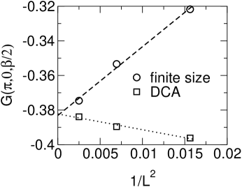
Figure 13: The imaginary time Green function $G({\bf{k}},\tau)$ at ${\bf{k}}=(\pi,0),\tau=\beta/2$ in the half-filled 2D Hubbard model, calculated with FSS/FLEX (circles) and DCA/FLEX (squares) when $U=1.57t$ for various cluster sizes $N_{c}=L\times L$). Both methods scale as $1/L^{2}$ and converge to a single value as $L\rightarrow\infty$. Taken from Aryanpour et al. (2003a).

This complementarity is also seen in results for the spectral gap in the 2D half-filled Hubbard model (see Huscroft et al., 2001 and Aryanpour et al., 2003a). In the DCA the gaps converge from small to large as the cluster size increases, while the converse occurs in FSS. Although we have only shown results of the DCA, we expect the CDMFT to show similar size dependence, since DCA and CDMFT share the same nature of the approximation (see discussion in Sec. II.3). Results obtained with the CPT algorithm however can be viewed to some extent as a periodic continuation of FSS. Thus it is an open question if the CPT method shows similar complementarity.

IV.2 2D Falicov-Kimball model

The usefulness of the discussed cluster theories was first demonstrated by the application of the DCA to the 2D FKM by Hettler et al. (1998, 2000). While the FKM is a particularly gentle test bed for novel approaches, it allows the study of the effects of non-local fluctuations.

The FKM can be considered as a simplified Hubbard model in which one spin species has zero hopping amplitude. The Hamiltonian reads

$$H=-t\sum_{<i,j>}d^{\dagger}_{i}d_{j}+U\sum_{i}(n^{d}_{i}-\frac{1}{2})(n^{f}_{i}-\frac{1}{2})\ ,$$ (186)

with $n^{d}_{i}=d^{\dagger}_{i}d^{\phantom{\dagger}}_{i}$ and $n^{f}_{i}=f^{\dagger}_{i}f^{\phantom{\dagger}}_{i}$. For a 2D square lattice the bandwidth of the noninteracting system is $W=8t$. At half filling and $D\geq 2$ the system has a second order phase transition from a homogeneous high temperature phase to a charge density wave with ordering vector ${\bf{Q}}=(\pi,\pi)$ for any nonzero $U$ Brandt and Schmidt (1986, 1987). The universality class is that of the 2D Ising model, the strong coupling limit $U/t\gg 1$ of the FKM.

Figure 14: DOS of the 2D FKM for a $4\times 4$–cluster at various temperatures calculated with DCA. The DOS develops a pseudogap as the temperature approaches $T_{c}\approx 0.189t$ ($U=4t$) due to the non-local CDW fluctuations present in the DCA $(N_{c}>1)$. In the DMFT ($N_{c}=1$), there is no $T$–dependence of the DOS above $T_{c}$. Figure from Hettler et al. (2000).

In Hettler et al. (2000) the FKM was evaluated within the DCA by a combination of QMC methods and exact enumeration for small clusters. Since the DMFT is a single-site theory ($N_{c}=1$), it yields an unphysical temperature-independent DOS of the mobile $d$-electrons Brandt and Mielsch (1989) due to the constraint of half filling (one electron per site of either the $d$ or $f$ variety). In a cluster theory with $N_{c}>1$ this artifact is absent, since a redistribution of Boltzmann weight with temperature is possible among the various configurations of $d$ or $f$ electrons on the cluster sites, while maintaining the condition of half filling on average. This temperature dependence is demonstrated in Fig. 14, where a pseudogap develops in the local DOS with decreasing temperature. This pseudogap can be interpreted as a precursor of the eventual transition to a CDW phase, which features a full gap at the Fermi level. In addition to the gap, there is fine structure in the DOS, related to an exchange energy $J_{eff}$. This is better observed in the momentum resolved spectral function (see Hettler et al., 2000; Laad and van den Bossche, 2000).

As stated above, the FKM has an instability to a phase with CDW order. As discussed in Sec. I.2, embedded cluster theories exhibit phase transitions at some temperature that, due to their residual mean-field character, lies above the exact $T_{c}$ of the infinite system. As the cluster size increases, one expects the effect of the mean-field to decrease, leading to a decreasing $T_{c}$ with increasing cluster size. The $N_{c}$ dependence of the transition temperature $T_{c}$ is shown in Fig. 15, together with a comparison with the $T_{c}$ obtained from FSS methods de Vries et al. (1993b, a); de Vries et al. (1994) and $T_{c}$ of the 2D Ising model with exchange coupling $J=1/(2U)$.The extrapolated cluster results agree with the FSS estimates and, for large values of $U$, also with the results obtained from the 2D Ising model. For smaller $U$ however, charge fluctuations begin to play a larger role, suppressing the $T_{c}$ compared to that of the Ising model which lacks charge fluctuations.

Figure 15: $T_{c}$ in the 2D FKM as a function of the inverse linear cluster size for $U/t=8,12,16$ calculated with DCA. The Ising limit, and FSS estimates of $T_{c}$ are shown for comparison. The inset shows that the influence of the cluster boundary conditions on $T_{c}$ disappears rapidly with increasing cluster size. Figure from Hettler et al. (2000).

The effect of different boundary conditions in the DCA cluster is illustrated in the inset. In small clusters the effect is strong, but already in a $6\times 6$- cluster the bulk of the cluster dominates and the boundaries play a minor role.

When $N_{c}=1$ only charge fluctuations with an energy scale $U$ are present. In a cluster theory the non-local “spin” fluctuations with an effective energy scale $J_{eff}$ ($\propto 1/2U$ for large $U$) must also be observable in thermodynamic quantities like the entropy and the specific heat. In Hettler et al. (2000) the entropy and specific heat was computed from the total energy of the cluster via a maximum-entropy method Huscroft et al. (2000). For better comparison, the calculations were performed in the uniform phase, even at temperatures below the CDW ordering $T_{c}$ by not allowing for the symmetry breaking. The results for a $2\times 2$- cluster are shown in Fig. 16, where the ratio of specific heat $C$ over the temperature $T$ is plotted for the DMFT and the DCA on a $2\times 2$- cluster. The appearance of the a second peak at lower temperature is a clear indication for the additional non-local fluctuations present on the cluster. The effect on the entropy is also strong, as shown in the inset.

Figure 16: Specific heat versus temperature for single site and $2\times 2$- clusters calculated with DCA and exact enumeration when $U=8t$. For $N_{c}=1$, there is a single peak with integrated weight $\ln(2)$ associated with the suppression of local charge fluctuations. For $N_{c}=4$, there is an additional peak at lower temperatures associated with critical fluctuations near the charge ordering transition temperature. $T_{c}$ for $N_{c}=4$ is indicated by an arrow. In the inset the entropy $S(T)=\int_{0}^{T}dT^{\prime}\frac{C(T^{\prime})}{T^{\prime}}$ is shown in units of $\ln(2)$. Figure from Hettler et al. (2000).

IV.3 1D Hubbard model

In this section we discuss the application of quantum cluster approaches to the 1D Hubbard model (in usual notation)

$${\cal H}=-t\sum_{i,\sigma}(c^{\dagger}_{i+1\sigma}c_{i\sigma}+h.c.)+U\sum_{i}n_{i\uparrow}n_{i\downarrow}\,,$$ (187)

which provides a non-trivial test ground for these techniques. In 1D quantum fluctuations are stronger than in higher dimensions. Hence quantum cluster approaches which cut off correlations beyond the length-scale set by the cluster size are expected to be less efficient than in higher dimensions. Therefore if quantum cluster approaches accurately describe the physics in 1D, they are highly likely to capture the physics in 2D and 3D. In addition, since the exact ground-state of the 1D Hubbard model is known from the Bethe ansatz solution Lieb and Wu (1968), a quantitative comparison of certain static quantities is possible. Fairly reliable results for dynamical quantities can be obtained from the density matrix renormalization method.

Bolech et al. (2003) applied the CDMFT/ED method to the 1D Hubbard model and systematically compared the results with those obtained from the DMFT and DMRG approaches. As an example of this study we show in Fig. 17 a comparison of the exact result with that obtained from DMFT (referred to as LISA for “Local Impurity Self-consistent Approximation”) and CDMFT for the single-particle spectral gap $\Delta(U)$ as a function of the on-site Coulomb repulsion $U$ in the half-filled case. The total number of sites in the effective cluster model including cluster and bath sites was fixed to six in the ED approach (see Sec. III.3.2).

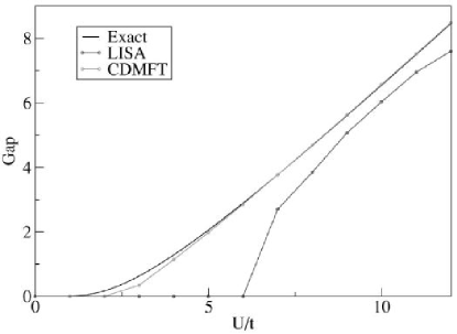
Figure 17: Spectral gap in the half-filled 1D Hubbard model as a function of $U/t$ calculated with DMFT (LISA) and CDMFT for a 2-site cluster, $N_{c}=2$ compared to the exact result. Taken from Bolech et al. (2003).

The behavior of the cluster results (CDMFT for $N_{c}=2$) is fundamentally different from the single-impurity result (LISA, $N_{c}=1$): When $N_{c}=1$, the spectral gap is reduced to values much smaller than the exact value and even vanishes at finite $U$. The existence of this Mott-transition in 1D for $N_{c}=1$ is a well known artifact of the DMFT method, reflecting the physics of infinite dimensions where the Mott-transition is indeed present Georges et al. (1996). In contrast, the $N_{c}=2$ result follows the exact result quite accurately yielding an insulating solution for all finite values of $U>0$ in agreement with the well known physics of the 1D model. This excellent reproduction of the exact gap for $N_{c}=2$ is quite encouraging since larger cluster sizes should produce even better results. And indeed, a comparison of the nearest neighbor Green function with DMRG results shows systematic improvements with increasing cluster size Bolech et al. (2003).

A related fundamental feature in 1D correlated systems is the breakdown of the Fermi-liquid picture because of spin-charge separation as described in the concept of Luttinger-liquids (see e.g. Voit, 1994). In a Fermi-liquid, the spectral weight $A({\bf{k}},\omega)$ is centered around a single quasiparticle peak at $\omega=\epsilon_{\bf{k}}$, while in a Luttinger-liquid, $A({\bf{k}},\omega)$ is distributed between two singularities associated respectively with spin- and charge-excitations (spinons and holons). Sénéchal et al. (2000) have calculated $A({\bf{k}},\omega)$ in the 1D Hubbard model using the CPT formalism. Fig. 18 shows a comparison of this quantity at the Fermi wave-vector $k=\pi/2$ as calculated by ordinary ED and its infinite lattice extension within the CPT method for various cluster sizes $N$ when $U=8t$ (bottom) and $U=16t$ (top).

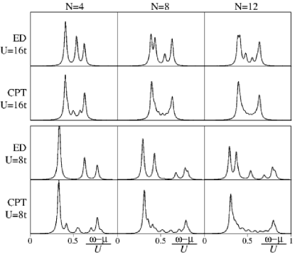
Figure 18: The spectral function $A(k,\omega)$ at $k=\pi/2$ in the half-filled 1D Hubbard model when $U=16t$ (top) and $U=8t$ (bottom), calculated with ordinary ED and with CPT for cluster sizes $N=4,8,12$. Taken from Sénéchal et al. (2000).

While no sign of spin-charge separation is seen in the pure ED results, the CPT method reveals the two branches of the spectral weight indicative of spin-charge separation. The two-peak structure resolves more clearly as the cluster size increases. Since propagation between clusters requires the spinon and holon to recombine, spin-charge separation can only exist on length- and time-scales limited by the cluster size. Consequently it takes fairly large clusters to clearly resolve this feature.

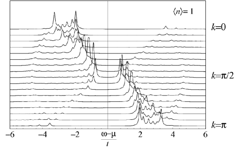
Figure 19: The spectral function $A(k,\omega)$ in the half-filled 1D Hubbard model when $U=4t$, calculated with CPT for $N_{c}=12$. Taken from Sénéchal et al. (2000).

The analysis of the $k$-dependent spectral function in Fig. 19 reveals the dispersion of the two branches. The spinon- and holon-branches show different dispersions and can be clearly identified together with the gap at the chemical potential at $k=\pi/2$. These $T=0$ simulations were extended to finite low temperatures $T>0$ by Aichhorn et al. (2003) who implemented a novel low-temperature Lanzcos algorithm which connects the exact ground-state Lanczos method with the established finite temperature Lanzcos method Jaklič and Prelovšek (2000). They showed that the spin-charge separation observed in the $T=0$ results persists at finite, low temperatures.

As exemplified by these studies, quantum cluster approaches have been proven very useful to explore the complex behavior of the 1D Hubbard model. Even studies with small cluster sizes are consistent with well-known results such as the opening of a Mott gap at half-filling for all $U>0$ and the existence of spin-charge separation reflected in the two branches in the electronic dispersion. This success in the 1D case shows great promise for applications of cluster methods in 2D or 3D where cluster methods are expected to be even more efficient since correlations are less pronounced.

IV.4 2D Hubbard model

The interest in the 2D Hubbard model (in usual notation)

$${\cal H}=\sum_{ij,\sigma}t_{ij}c^{\dagger}_{i\sigma}c_{j\sigma}+U\sum_{i}n_{i\uparrow}n_{i\downarrow}$$ (188)

has been revived recently in particular since it is believed to capture the physics of the superconducting planes in high-temperature superconductors (HTSC) (Anderson, 1997b; Zhang and Rice, 1988, 1990). This section reviews various applications of quantum cluster approaches to the 2D Hubbard model at half-filling and at finite doping, including results for a possible Mott-Hubbard transition, antiferromagnetism and its precursors, pseudogap phenomena and superconductivity.

IV.4.1 Metal-insulator transition

The study of a possible metal-insulator transition (MIT) in the 2D Hubbard model at half-filling ($\epsilon_{o}=t_{ii}=-U/2$) is under active research. This problem was studied in the unfrustrated model, i.e. with only nearest neighbor hopping $t_{ij}=\epsilon_{o}\delta_{ij}-t\delta_{\langle ij\rangle}$ within DCA/QMC by Moukouri and Jarrell (2001) and with the two-site composite operator method (see Sec. II.8) by Stanescu and Phillips (2001). The frustrated case (additional next-nearest neighbor hopping $t^{\prime}\delta_{\langle\langle ij\rangle\rangle}$) was investigated by Parcollet et al. (2003).

Numerical calculations have shown that the ground state of the unfrustrated model is an antiferromagnetic insulator with the Néel temperature $T_{\rm N}=0$ constrained by the Mermin-Wagner theorem. A spectral gap hence exists at $T=0$. However the central question about the origin of the gap and its relation to antiferromagnetic ordering is less understood. Is the gap a direct consequence of the antiferromagnetic ordering at $T=0$ or does it arise from strong correlations at higher temperatures?

To appreciate the significance of this issue it is important to understand the fundamental difference between antiferromagnetic insulators, i.e. insulators due to magnetic ordering and Mott insulators, i.e. insulators due to electronic correlations. Antiferromagnetic insulators result from the doubling of the unit cell in the ordered state and are therefore adiabatically connected to band insulators which have an even number of electrons per unit cell. In contrast, paramagnetic Mott insulators have an odd number of electrons per unit cell and are therefore fundamentally different from band insulators.

At strong coupling ($U\gg W$) the situation is well understood: A charge gap of order $U$ develops in the spectrum below temperatures $T\approx U$ due entirely to strong electronic correlations. The spins are coupled by the exchange interaction $J=4t^{2}/U$ and govern the low-energy physics. As a result spin and charge are separated. Systems in this regime are hence Mott insulators and the antiferromagnetic ordering at $T=0$ is merely the result of the Mott-transition at higher temperatures.

Different scenarios however exist for the weak-coupling regime ($U\ll W$): In the weak coupling point of view, a spin density wave forms at $T=0$ due to the nesting of the Fermi surface and leads to the doubling of the unit cell. Hence the gap in the spectrum is a direct consequence of the antiferromagnetism at $T=0$. This perturbative point of view is referred to as Slater mechanism. It is in contrast to the second opinion due to Anderson (1997a, b) who has argued that the 2D half-filled Hubbard model is always in the strong-coupling regime, so that a Mott gap is present for all $U>0$ as in 1D (see Sec. IV.3). As the temperature decreases, local moments develop because of the opening of the Mott gap which then order at $T=0$. Thus the antiferromagnet at $T=0$ is a consequence of the Mott transition.

The MIT in the half-filled Hubbard model has been extensively studied within the DMFT (for a review see Georges et al., 1996). In the DMFT one can easily disentangle the effects leading to antiferromagnetic and Mott gaps. The DMFT equations for the paramagnetic state of the bipartite Bethe lattice are identical with the equations of the fully frustrated infinite dimensional model Georges et al. (1996). This justifies the study of the paramagnetic solution within the antiferromagnetic phase of the unfrustrated model which shows a first order Mott MIT ending at a finite temperature critical point Georges et al. (1996). Although this justification does not hold for $N_{c}>1$, one can still study the paramagnetic solution by enforcing the spin symmetry and hence avoiding the opening of a full spectral gap due entirely to magnetic ordering. Following this approach, Moukouri and Jarrell (2001) studied the MIT in the unfrustrated 2D half-filled Hubbard model using DCA/QMC systematically as a function of cluster size $N_{c}$. The MIT can be identified by analyzing the behavior of the double occupancy $\langle D\rangle=\langle n_{\uparrow}n_{\downarrow}\rangle$. This quantity is shown in Fig. 20 for different values of the Coulomb repulsion $U$ and cluster size $N_{c}$.

Figure 20: Double occupancy as a function of temperature for different values of $U$ in the half-filled 2D Hubbard model calculated with DCA/QMC for various cluster sizes $N_{c}$. Here, $t=0.25$, so the lines for $U=0.5,1,2$ correspond to $U/t=2,4,12$. Taken from Moukouri and Jarrell (2001).

When $N_{c}=1$ the double occupancy displays evidence for a MIT when $U$ is of the order of the bandwidth $W=8t=2$: $\langle D\rangle$ is monotonically increasing with temperature when $U=3$, but displays a minimum for $U=0.5$ and $1$ indicating the emergence of quasiparticle states at the chemical potential at low temperatures. When $N_{c}>1$ the situation is radically different: In the strong coupling regime ($U=3$), local fluctuations dominate and $\langle D\rangle$ is essentially independent of $N_{c}$ except at very low temperatures. In contrast, in the weak coupling regime, the minimum found for $N_{c}=1$ flattens progressively as $N_{c}$ increases from 8 to 16. When $N_{c}\geq 36$ a downturn in $\langle D\rangle$ appears at low temperatures. By opening a gap and hence localizing the moments, the system can gain free energy by taking advantage of the short-ranged magnetic correlations.

Figure 21: DOS when $U/t=4$ for different temperatures in the half-filled 2D Hubbard model calculated with DCA/QMC for various cluster sizes $N_{c}$. Taken from Moukouri and Jarrell (2001).

The results for the DOS shown in Fig. 21 support the evidence from the double occupancy. The quasiparticle Kondo-like resonance at the chemical potential for $N_{c}=1$ is destroyed by non-local correlations when $N_{c}>1$. As $N_{c}$ increases, a gap opens at the chemical potential and the Hubbard sidebands become more pronounced consistent with the suppression of $\langle D\rangle$. Given the fact that DCA always underestimates correlation induced spectral gaps (see Sec. IV.1), these simulations indicate the absence of a weak-coupling regime in the unfrustrated 2D Hubbard model at half-filling consistent with Anderson’s point of view.

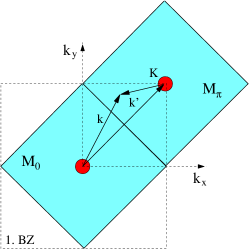
Figure 22: Tiling of the first Brillouin zone for $N_{c}=2$.

Another interesting aspect is whether this result changes at zero temperature, $T=0$ and the MIT predicted by DMFT returns. As evidence that even at $T=0$ one must expect a gap in the spectra for any $U>0$, we show here first DCA results at $T=0$ obtained with Wilson’s NRG for a cluster size of $N_{c}=2$. The appropriate tiling of the Brillouin zone is shown in Fig. 22 and the resulting coarse-grained spectral functions $\bar{A}({\bf{K}},w)=-\frac{1}{\pi}\Im m\bar{G}({\bf{K}},w)$ for the two cluster ${\bf{K}}$-points are shown in Fig. 23.

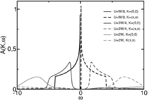
Figure 23: DCA coarse-grained spectral functions for different values of $U$ obtained from $N_{c}=2$ DCA/NRG calculations at $T=0$. Apparently, no finite critical value of $U$ for a conventional Mott-Hubbard transition seems to exist. In contrast, for all $U>0$ a gap exists at the Fermi energy.

Even for small values of $U$ a well defined gap exists in the spectrum at the Fermi energy. Note that all calculations were done in the paramagnetic phase, i.e. the concept of a Slater insulator does not apply here. The gap quickly increases with increasing $U$ and at the same time the system gains more spectral weight in the incoherent parts of the spectrum, i.e. begins to resemble what one expects from Mott localized states.

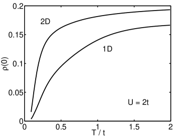
Figure 24: DOS as a function of temperature at the chemical potential in the 1D and 2D half-filled Hubbard model when $U=2t$ calculated with a two-site composite operator approximation. Taken from Stanescu and Phillips (2001).

The DCA results were confirmed in a similar cluster study by Stanescu and Phillips (2001) using the two-site composite operator method discussed in Sec. II.8. Figure 24 shows the results of this study for the temperature dependence of the value of the DOS at the chemical potential, $\rho(0)$ in the 1D and 2D models for small $U=2t$. As a consequence of the shape of the non-interacting DOS, the 2D result for $\rho(0)$ is enhanced over the 1D result. However, in both 1D and 2D, $\rho(0)$ falls to zero as the temperature decreases indicating the absence of a metallic state at half-filling even for small $U$.

To elucidate the role of antiferromagnetic correlations in the opening of the Mott gap, the frustrated Hubbard model may be studied. In the $t$-$t^{\prime}$ Hubbard model, a next-nearest neighbor hopping $t^{\prime}$ between sub-lattices strongly frustrates antiferromagnetic correlations. This model was studied by Parcollet et al. (2003) for $t^{\prime}=t$ on a $2\times 2$ cluster using CDMFT/QMC. We reproduce their results for the $U$ dependence of the double occupancy $d_{occ}=1/4\sum_{i=1}^{4}\langle n_{i\uparrow}n_{i\downarrow}\rangle$ for different temperatures in Fig. 25. Similar to the behavior found in DMFT, $d_{occ}$ displays a downturn at a critical value $U_{c}$, indicating a transition from a metallic to an insulating state. An inspection of the spectral weight $A({\bf{k}},0)$ at the chemical potential reveals that the gap opens first in the region around ${\bf{k}}=(\pi,0)$ Parcollet et al. (2003).

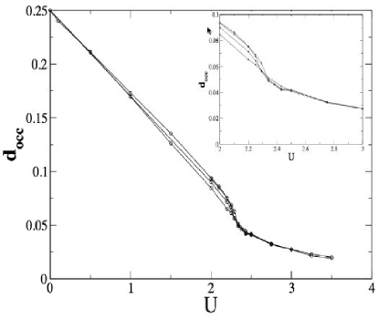
Figure 25: Double occupancy as a function of $U$ in the frustrated 2D Hubbard model with $t^{\prime}=t$ for different temperatures (from top to bottom) $T/t=1/5,4/30,1/10,1/11$, calculated with CDMFT/QMC. Taken from Parcollet et al. (2003).

These results were substantiated by a CPT study of the frustrated 2D Hubbard model Sénéchal and Tremblay (2003) for $t^{\prime}=-0.4t$. Although not the focus of this study, the results show further evidence of a Mott transition at a finite value of $U$ in the filling dependence of the chemical potential.

The existence of the Mott transition in the frustrated Hubbard model and its absence in the unfrustrated model seems to indicate that antiferromagnetic correlations play a key role in the opening of a Mott gap at weak coupling. Since the opening of the gap occurs in the paramagnetic solution, it cannot be attributed to the existence of antiferromagnetic ordering. Thus the conclusion reached from these cluster studies is that a symbiosis of local moment formation and short-ranged antiferromagnetic correlations cause the gap to open at finite temperatures Moukouri and Jarrell (2001).

IV.4.2 Antiferromagnetism and precursors

If the simulations are performed without enforcing the spin symmetry or frustrating the lattice, the system is given the possibility to transform to a state with antiferromagnetic order. Since the system is two-dimensional, we know from the Mermin-Wagner theorem that the true Néel temperature $T_{\rm N}$ is necessarily zero. As found in infinite dimensions Jarrell et al. (1993), the DMFT predicts a finite temperature transition even in 2D due to its mean-field character. As discussed in Sec. I.2, cluster approaches restore non-local fluctuations and thus are expected to drive the Néel temperature systematically to zero as the cluster size increases.

As discussed in Secs.  II.6 and II.5, phase transitions can be identified from the disordered (here: paramagnetic) state by calculating the corresponding susceptibility, or from the ordered state by computing the order parameter. The calculation of order parameters is exemplified in Fig. 26 where we plot the DCA/NCA result for the sub-lattice magnetization $m=1/N\sum_{i,\sigma}e^{i{\bf{Q}}\cdot{\bf x}_{i}}\sigma n_{i\sigma}$ (see Eq. (II.5.3)) as a function of the reduced temperature $t=T/T_{\rm N}$ in the 2D half-filled Hubbard model for the cluster sizes $N_{c}=1$ and $N_{c}=4$ when $U=4t$. The $N_{c}=4$ Néel temperature $T_{\rm N}=0.208t$ is reduced from the $N_{c}=1$ result $T_{\rm N}=0.304t$ and the order parameter is strongly suppressed. As expected, non-local spin fluctuations suppress antiferromagnetism.

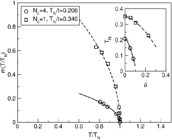
Figure 26: Sublattice magnetization as a function of temperature in the half-filled 2D Hubbard model calculated with DCA/NCA for cluster sizes $N_{c}=1,4$ when $U=4t$. Inset: Neél-temperature versus doping. Taken from Maier (2001).

Figure 27 shows the DCA/QMC result for the temperature dependence of the inverse antiferromagnetic susceptibility $1/\chi_{AF}$ at $U=6t$ for various cluster sizes $N_{c}$ in the paramagnetic state. At high temperatures the susceptibility is independent of $N_{c}$ due to the lack of non-local fluctuations. In contrast to FSS, the low temperature susceptibility diverges at $T=T_{\rm N}$ indicating the instability to the antiferromagnetic state. When $N_{c}=1$ the susceptibility diverges with a critical exponent $\gamma\approx 1$ as expected for a mean-field theory. Consistent with the NCA results the susceptibility diverges at lower temperatures when $N_{c}>1$ with larger exponents indicative of fluctuation effects. However as discussed in Sec. I.2 these critical exponents reflect the behavior at intermediate temperatures. Very close to the transition, there must a region of mean-field behavior. However, this region is very difficult to resolve with DCA/QMC, due to numerical noise, which is especially large near the transition.

Figure 27: Inverse antiferromagnetic susceptibility versus temperature in the half-filled 2D Hubbard model calculated with DCA/QMC for various cluster sizes $N_{c}$ when $U=6t$. The lines are fits to the function $(T-T_{\rm N})^{\gamma}$. Inset: Corresponding Neél-temperatures as a function of the cluster size. Taken from Jarrell et al. (2001b).

As shown in the inset, the transition temperatures fall very slowly with the cluster size $N_{c}$, but the $N_{c}=4$ falls off the curve. As detailed in Sec. II.3.4, fluctuation effects in clusters with linear size $L=2$ are over-proportionally enhanced since its coordination number is reduced compared to the original system. Hence the $N_{c}=4$ result does not fall on the curve, similar to the behavior seen in DCA studies of the FKM Hettler et al. (2000).

The question arises of whether the same non-local fluctuations which are responsible for suppressing the antiferromagnetism result in precursers of the antiferromagnetic phase transition. The onset of antiferromagnetic correlations on short time- and length-scales may be signaled by a pseudogap in the DOS as a precursor to the antiferromagnetic gap. This was predicted by Kampf and Schrieffer (1990) using a phenomenological ansatz for the weak coupling Hubbard model based on the presence of strong antiferromagnetic spin-fluctuations. On a microscopic level, this question has been addressed by FSS/QMC in the 2D Hubbard model in Vekic and White (1993) and Creffield et al. (1995) and by approximate many-body techniques in Deisz et al. (1996) and Moukouri et al. (1999). But the results have been inconclusive as to the existence of a pseudogap at low temperatures, due to the limitations of these techniques.

Within quantum cluster approaches the pseudogap phenomenon was first studied by Maier et al. (2000b) within the DCA/NCA formalism. In contrast to $N_{c}=1$ where a Kondo-like quasiparticle peak emerges at the chemical potential as the temperature is decreased (reminiscent of the $D=\infty$ DMFT result Georges et al. (1996)), a pseudogap was found when non-local correlations were included in $N_{c}=4$ simulations.

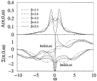
Figure 28: Spectral function $A({\bf{k}},\omega)$ and the real $\Re e\Sigma({\bf{k}},\omega)$ and imaginary $\Im m\Sigma({\bf{k}},\omega)$ parts of the self-energy for various temperatures at ${\bf{k}}=(\pi,0)$ in the 2D half-filled Hubbard model for $U=5.2t$ calculated with DCA/QMC for a 64-site cluster ($N_{c}=64$). Taken from Huscroft et al. (2001).

For larger cluster sizes, the emergence of the pseudogap in the DOS was explored by DCA/QMC in Huscroft et al. (2001) and DCA/FLEX in Aryanpour et al. (2003a). Figure 28 displays the DCA/QMC results for the spectral function $A({\bf{k}},\omega)$ and the self-energy $\Sigma({\bf{k}},\omega)$ at the Fermi wave-vector ${\bf{k}}=(\pi,0)$ in the paramagnetic state for a 64-site cluster ($N_{c}=64$) at various temperatures. With decreasing temperature a pseudogap develops in $A({\bf{k}},\omega)$ at the Fermi wave-vector ${\bf{k}}=(\pi,0)$. Simultaneously the slope of $\Re e\Sigma({\bf{k}},0)$ becomes positive at ${\bf{k}}=(\pi,0)$ signaling the appearance of two new solutions in the quasiparticle equation $\omega-\epsilon_{\bf{k}}+\mu-\Re e\Sigma({\bf{k}},\omega)=0$. In addition to the strongly damped solution at $\omega=0$ which is also present in the non-interacting system these two new quasiparticle solutions appear on both sides of $\omega=0$. A consequence of the antiferromagnetic order on short time- and length-scales, they can be viewed as precursers of the doubling of the unit cell in the antiferromagnetic state. The pseudogap is generated by the local minimum in $\Im m\Sigma({\bf{k}},\omega)$ which signals the breakdown of Fermi-liquid behavior.

By studying the system on a triangular lattice, Imai and Kawakami (2002) investigated the effects of frustration on the pseudogap in the half-filled 2D Hubbard model using the DCA/NCA and DCA/FLEX approaches. Figure 29 schematically illustrates the triangular lattice and the choice of cluster wave-vectors in the corresponding Brillouin zone for $N_{c}=4$.

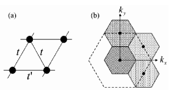
Figure 29: Illustration of the triangular lattice with hopping amplitudes $t$ and $t^{\prime}$ (a) and DCA coarse-graining cells (b) in the first Brillouin zone (dashed line) of the triangular lattice when $N_{c}=4$. Cluster ${\bf{K}}$-points are indicated by the dots. Taken from Imai and Kawakami (2002).

For $t^{\prime}=0$ this setup corresponds to the unfrustrated system and the effects of frustration can be systematically studied as $t^{\prime}$ is increased to its maximal value $t^{\prime}=t$. Figure 30 reproduces the results for the DOS and coarse-grained spectra $\bar{A}({\bf{K}},\omega)$ for different values of the frustration $t^{\prime}$.

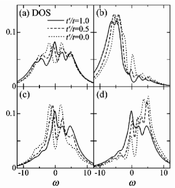
Figure 30: The DOS (a) and coarse-grained single-particle spectral functions $\bar{A}({\bf{K}},\omega)$ in the 2D half-filled frustrated Hubbard model for ${\bf{K}}=(0,0)$ (b), ${\bf{K}}=(\pi,\pi/\sqrt{3})$ (c) and ${\bf{K}}=(0,2\pi/\sqrt{3})$ (d) for various values of the frustration $t^{\prime}$ when $U=6t$ and $T=0.6t$. Taken from Imai and Kawakami (2002).

As the geometrical frustration increases from $t^{\prime}=0$ to $t^{\prime}=t$, antiferromagnetic spin fluctuations are suppressed. Consequntly the pseudogap in the unfrustrated system diminishes and a quasiparticle peak develops at the chemical potential. The change in the DOS mainly originates in the region in momentum space around ${\bf{K}}=(\pi,\pi/\sqrt{3})$ where the Fermi surface is located. These results are thus consistent with an antiferromagnetic spin fluctuation driven pseudogap.

IV.4.3 Pseudogap at finite doping

The properties of the Hubbard model away from half-filling are of great interest especially in the context of HTSC. Contrary to Fermi-liquid theory, low-energy spin-excitations in HTSC are suppressed at low temperatures as evidenced by Knight-shift experiments. Concomitantly, the Fermi surface is gapped along certain directions in the Brillouin zone as indicated in ARPES experiments. This pseudogap phenomenon has proven a great challenge for theories of strongly correlated systems.

DMFT has provided great insight into the evolution of spectra in doped Mott-insulators. Exact results based on the self-consistent mapping onto an Anderson impurity model show that the system is a Fermi-liquid in the metallic state in the absence of symmetry breaking below a coherence temperature reminiscent of the Kondo-temperature Georges and Kotliar (1992). Hence the spin-susceptibility becomes finite at low temperatures in contrast to the experimental results in underdoped cuprates. Furthermore Müller-Hartmann (1989a) showed that because the self-energy is momentum independent, volume and shape of the Fermi surface are identical to the non-interacting Fermi-surface. Thus DMFT does not include the effects that lead to the emergence of a pseudogap in the spin- and quasiparticle spectrum and cluster extensions are necessary.

Within quantum cluster approaches the pseudogap phenomenon in the doped 2D Hubbard model was studied with DCA/NCA in Maier et al. (2000b) and Maier (2001), with DCA/QMC in Jarrell et al. (2001a) and Maier et al. (2002a), with the two-site composite operator method in Stanescu and Phillips (2003b, a) and with the CPT in Sénéchal and Tremblay (2003).

Figure 31 shows the DCA/NCA result for the low-energy DOS in the 2D Hubbard model at 5% doping ($\delta=0.05$) around the chemical potential ($\omega=0$) calculated on a 4-site cluster ($N_{c}=4$). At high temperature $T>0.3t$ no pseudogap is seen in the DOS. As the temperature is lowered the DOS distorts at the chemical potential and a pseudogap emerges at $\omega=0$ when $T\lesssim 0.3t$.

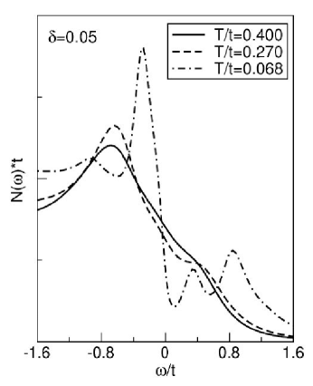
Figure 31: DOS for various temperatures in the 2D Hubbard model at 5% doping when $U=12t$ near the chemical potential ($\omega=0$) calculated with DCA/NCA for a 4-site cluster, $N_{c}=4$. Taken from Maier (2001).

These perturbative results were confirmed in DCA/QMC simulations by Jarrell et al. (2001a) which we reproduce in Fig. 32. At low temperatures a pseudogap is observed in the DOS at dopings $\delta\lesssim 0.2$. This depression of quasiparticle states at the chemical potential is accompanied by a downturn of the uniform magnetic susceptibility shown in the inset. For low to intermediate doping it develops a maximum defining a crossover temperature $T^{*}$. Below $T^{*}$ quasiparticle and low-energy spin excitations are suppressed by non-local correlations similar to what is observed in the experiment.

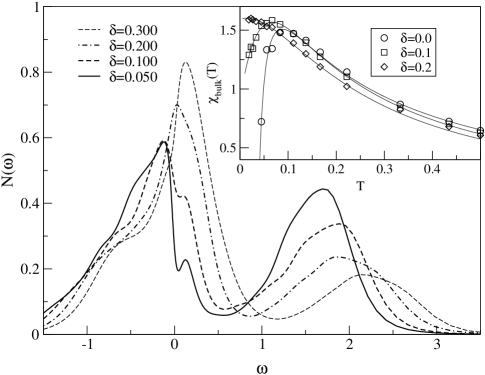
Figure 32: DOS for various dopings $\delta$ in the 2D Hubbard model at $T=0.092t$ and $U=8t$ calculated with DCA/QMC for a 4-site cluster, $N_{c}=4$. Inset: Uniform spin-susceptibility as a function of temperature. Taken from Jarrell et al. (2001a).

At the same time, the charge susceptibility (not shown) displays qualitatively different behavior forming a strong low-energy peak at low temperatures (see Maier et al., 2002a; Maier et al., 2004 and Fig. 38) which signals the emergence of coherent charge excitations below $T^{*}$. The $N_{c}=4$ DCA results are thus consistent with a spin-charge separated picture as in Anderson’s RVB theory. This is not surprising since, as we discussed in Sec. IV.4.2, fluctuations are enhanced in the $N_{c}=4$ cluster due to the “too small” coordination number. It is known that small coordination numbers favor the spin-charge separated RVB state Anderson (1987) over the Néel state. Indeed the RVB state was shown to be the ground state of a 2$\times$2 Heisenberg model with periodic boundary conditions with a large gap to the first excited state Dagotto and Moreo (1988).

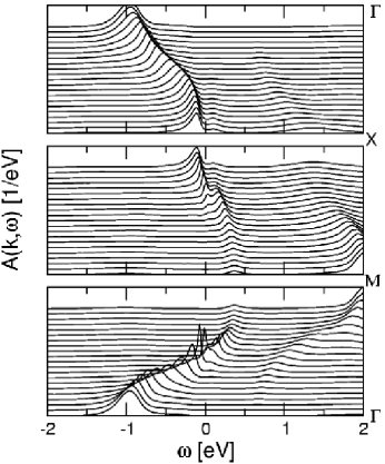
Figure 33: The spectral function $A({\bf{k}},\omega)$ near the chemical potential in the 2D Hubbard model at $T=0.088t$ and $U=8t$ along high-symmetry directions in the first Brillouin-zone between $\Gamma=(0,0)$, $X=(\pi,0)$ and $M=(\pi,\pi)$ calculated with DCA/QMC for a 4-site cluster $N_{c}=4$.

The corresponding 4-site DCA/QMC result for the momentum resolved spectral function $A({\bf{k}},\omega)$ in the pseudogap regime is displayed in Fig. 33 for energies near the chemical potential between points of high symmetry $\Gamma=(0,0)$, ${\rm X}=(\pi,0)$ and ${\rm M}=(\pi,\pi)$ in the first Brillouin zone. The overall dispersion of the band crossing the chemical potential $\omega=0$ follows that of the non-interacting system $\epsilon_{\bf{k}}$. While coherent quasiparticles exist along $\Gamma\rightarrow{\rm M}$, the pseudogap is seen near ${\rm X}=(\pi,0)$ at the chemical potential $\omega=0$. The anisotropy of the pseudogap is thus consistent with that observed in ARPES measurements on underdoped hole-doped cuprates.

Qualitatively similar results for the emergence of the quasiparticle spectrum in the doped 2D Hubbard model were obtained by Stanescu and Phillips (2003b) using the two-site composite operator approach discussed in Sec. II.8 (see also Stanescu and Phillips, 2003a). Figure 34 illustrates their results for the doping dependence of the chemical potential $\mu$, the imaginary part of the self-energy $\Im m\Sigma$ and the $U$ dependence of the low-energy DOS.

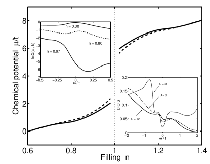
Figure 34: The doping dependence of the chemical potential in the 2D Hubbard model calculated with the two-site composite operator method for $T=0.15t$ (dashed line) and $T=0.07t$ (solid line). Right inset: DOS for various values of $U$ at 5% doping ($n=0.95$). Left inset: Imaginary part of the self-energy evaluated at a Fermi momentum (0.3,2.10) for $n=0.97$, (0.3,1.84) for $n=0.80$ and (0.3,1.06) for $n=0.3$. Taken from Stanescu and Phillips (2003b).

At half-filling the chemical potential has a discontinuity indicating the absence of mid-gap states. In agreement with DCA/QMC Jarrell et al. (2001a, b) and DCA/NCA Maier (2001) results, $|\Im m\Sigma|$ is large in the underdoped pseudogap regime ($n=0.97$) and acquires Fermi-liquid behavior at larger doping $n\leq 0.80$ indicated by the parabolic minimum at the chemical potential. As illustrated in the inset, the depth of the pseudogap decreases as $U$ increases suggesting a pseudogap scale compatible with $t^{2}/U$.

Sénéchal and Tremblay (2003) recently investigated the difference in pseudogap behavior between electron and hole doped HTSC using CPT for the 2D $t-t^{\prime}-t^{\prime\prime}$ Hubbard model. As illustrated in the Fermi-surface plots in Fig. 35, their results at $U=8t$ demonstrate that the pseudogap in hole-doped systems (right side) occurs near ${\rm X}=(\pi,0)$ at optimal doping consistent with the results discussed above. In electron-doped systems (left side) however, the pseudogap appears at the crossing points of the Fermi surface with the antiferromagnetic Brillouin zone boundary at moderate interaction $U=4t$. When $U$ is large however (not shown), the Fermi surface only survives in the neighborhood of $(\pi,0)$ and $(0,\pi)$. As shown in the lower panels of Fig. 35 the pseudogap in both cases is generated by a large scattering rate $|\Im m\Sigma({\bf{k}},0)|$ at the chemical potential.

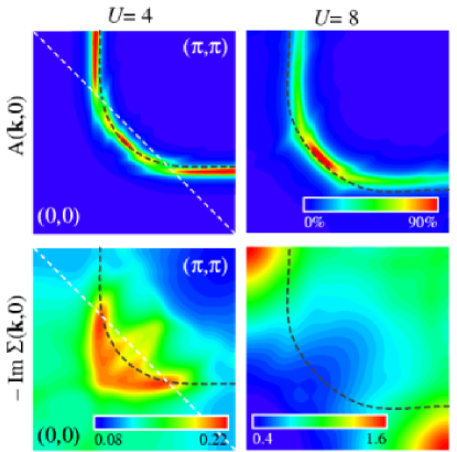
Figure 35: Intensity plot of the spectral function $A({\bf{k}},0)$ (top) and imaginary part of the self-energy $\Im m\Sigma({\bf{k}},0)$ (bottom) of the 2D Hubbard model calculated with CPT on a $3\times 4$-site cluster. The left side shows the results in the first quadrant of the Brillouin zone for the 17% electron-doped system at $U=4t$ and the right side for the 17% hole-doped system at $U=8t$. Taken from Sénéchal and Tremblay (2003).

A unified picture of the spectral properties of the electron- and hole-doped cuprates thus emerges from these results if the interaction strength $U$ is allowed to be doping dependent. To reproduce the experimental observations in optimally doped cuprates, large values of $U$ seem necessary in hole-doped ($U\approx 8t$) systems, while smaller values of $U$ describe the electron-doped systems ($U\lesssim 6t$) Sénéchal and Tremblay (2003).

IV.4.4 Superconductivity

FSS QMC simulations for the doped 2D Hubbard model in the intermediate coupling regime $U\sim W$ support the idea of a spin-fluctuation driven interaction mediating $d$-wave superconductivity (for a review see Scalapino, 1999). However the fermion sign problem limits these calculations to temperatures too high to study a possible transition. These calculations are also restricted to relatively small system sizes, making statements for the thermodynamic limit problematic, and inhibiting studies of the low-energy physics. These shortcomings do not apply to embedded cluster theories which are built for the thermodynamic limit. Cluster sizes larger than one are necessary however, to describe a possible transition to a state with a non-local ($d$-wave) order parameter as discussed in Sec. II.5.

It is well known from weak coupling FSS FLEX results Bickers et al. (1989) and phenomenological theories Monthoux et al. (1991); Scalapino (1999) that antiferromagnetic spin-fluctuations mediate pairing with $d$-wave symmetry and cause a pseudogap in underdoped systems. In optimally doped cuprates, these spin-fluctuations are known to be short-ranged, extending over a few lattice spacings. Hence quantum cluster approaches should provide an adequate methodology to study superconductivity in these systems. Pairing in the 2D Hubbard model was studied using DCA/NCA by Maier et al. (2000a), and with DCA/QMC by Jarrell et al. (2001a, b) and Maier et al. (2004). The possible coexistence of superconductivity with antiferromagnetic order was investigated by Lichtenstein and Katsnelson (2000).

The results of 4-site ($N_{c}=4$) DCA simulations for the doped 2D Hubbard model show an instability to a superconducting phase with a $d_{x^{2}-y^{2}}$-wave order parameter at low enough temperatures. As a typical example of this transition, Fig. 36 shows the DCA/NCA result for the DOS and the coarse-grained anomalous Green function $\bar{G}_{12}({\bf{K}},\omega)\equiv{\bar{F}}({\bf{K}},\omega)$ defined in Eq. (97) at different cluster ${\bf{K}}$-points near the chemical potential in the superconducting state.

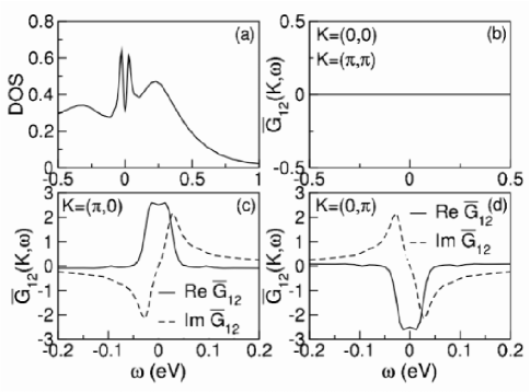
Figure 36: DOS near the chemical potential (a) and coarse-grained anomalous Green function $\bar{G}_{12}({\bf{K}},\omega)\equiv\bar{F}({\bf{K}},\omega)$ for different DCA cells (b-c) in the superconducting state of the 2D Hubbard model at 19% doping, $T=0.047t$, $U=12t$ calculated with DCA/NCA for a 4-site cluster, $N_{c}=4$. Taken from Maier et al. (2000a).

$\bar{G}_{12}({\bf{K}},\omega)$ vanishes at the cluster ${\bf{K}}=(0,0)$ and $(\pi,\pi)$ but is finite at $(\pi,0)$ and $(0,\pi)$ with opposite signs. Since the ${\bf{K}}$-dependence of the coarse-grained order parameter ${\bar{\Delta}}_{\bf{K}}$ is given by the ${\bf{K}}$-dependence of the coarse-grained anomalous Green function (see Eq. (101)), this result is consistent with a $d_{x^{2}-y^{2}}$-symmetry of the order parameter. The finite pair amplitude is also reflected in the DOS depicted in the upper left part where the lower subband of the full spectrum is shown. It displays the superconducting pseudogap at zero frequency as expected for a $d$-wave order parameter.

Jarrell et al. (2001a, b) used DCA/QMC to search for many different types of superconductivity, including $s$-, extended $s$-, $p$- and $d$-wave, of both even and odd frequency. Of these, only the odd-frequency $s$-wave and even-frequency $d$-wave pair-field susceptibilities were strongly enhanced, and only the $d$-wave susceptibility diverged.

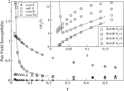
Figure 37: Pair-field susceptibilities versus temperature in the even frequency $s$-wave, extended $s$-wave ($xs$), $d$-dave and odd-frequency $s$-wave channels in the 2D Hubbard model at 5% doping, $U=8t$ calculated with DCA/QMC for a 4-site cluster, $N_{c}=4$. Inset: Inverse $d$-wave pair-field susceptibility versus temperature for different dopings and cluster sizes. The line is a fit to $b(T-T_{c})^{\gamma}$ with $T_{c}=0.084t$ and $\gamma=0.72$. Taken from Jarrell et al. (2001a).

This is illustrated in Fig. 37 where the pair-field susceptibilities are plotted versus temperature at 5% doping. The behavior of the inverse $d$-wave pair-field susceptibility as a function of temperature for $N_{c}=1$ and 4 and $\delta=0$ and 0.5 is shown in the inset. For $N_{c}=1$ there is no tendency towards pairing. As detailed in Sec. II.5, the DMFT is not able to describe pairing with symmetries lower than the lattice symmetry (i.e., $p$-, $d$-wave, etc.). For $N_{c}=4$ and $\delta=0$ the inverse susceptibility rises abruptly as the temperature is lowered and the Mott gap opens in the DOS. The Mott gap becomes more pronounced as $N_{c}$ increases (see Sec. IV.4.1), so that for larger clusters the gap prevents superconductivity even for $U<W$. If charge excitations are gapped, then pairing is suppressed. At half-filling, for $U=8t$ the gap is of order $U$, and thus much larger than the magnetic exchange energy $J\sim 4t^{2}/U=0.5t$. Hence the opening of the Mott gap suppresses any magnetically mediated pairing. Away from half-filling the width of the pseudogap in the charge excitation spectrum is much smaller, of the order of $J$ (see Sec. IV.4.3), so that magnetically mediated pairing is possible.

More insight in the nature of pairing was gained from further DCA/QMC studies of the 2D Hubbard model Maier et al. (2004).

Figure 38: DOS (left), local dynamic spin susceptibility (center) and local dynamic charge susceptibility (right) in the 2D Hubbard model at 5% doping at different temperatures above and below the critical temperature $T_{c}=0.0218=0.087t$ calculated with DCA/QMC for a 4-site cluster, $N_{c}=4$. Taken from Maier et al. (2004).

Figure 38 shows the DCA/QMC result for the evolution of the DOS, the local dynamic spin- and local dynamic charge-susceptibility as the temperature decreases below the critical temperature $T_{c}$. As discussed in Sec. IV.4.3, the normal state low-temperature DOS and spin-susceptibility display a pseudogap, i.e. a depression of low-energy quasiparticle and spin excitations. Both quantities evolve smoothly across the superconducting transition with the pseudogap changing to a superconducting gap below $T_{c}$. However since the charge susceptibility is peaked at zero frequency even slightly above $T_{c}$, it changes abruptly upon pairing to show the same behavior as the spin-susceptibility, including the superconducting gap at low frequencies. Remarkably, well below $T_{c}$ all quantities display narrow peaks at $\omega\approx 0.1{\rm eV}$, delimiting the superconducting gap. This result clearly indicates the formation of quasiparticles below $T_{c}$. The absence of quasiparticles in the normal state however undermines the very foundation of the BCS theory of conventional superconductors where pairing is a result of a Fermi surface instability that relies on the existence of quasiparticles in a Fermi-liquid Schrieffer (1993).

DCA/QMC results for the condensation energy further establish the unconventional character of superconductivity in the 2D Hubbard model Maier et al. (2004). Figure 39 presents the kinetic (top) and potential (bottom) energies, ${\rm Tr}({\bf t}{\bf G})$ and ${\rm Tr}({\bf\Sigma}{\bf G})$ respectively, of the superconducting (SC) and normal state (NS) solution as a function of temperature at low doping $\delta=0.05$ (left) and optimal doping $\delta=0.20$ (right).

Figure 39: Kinetic (top) and potential (bottom) energies versus temperature in the normal (NS) and superconducting (SC) states in the 2D Hubbard model at 5% (left) and 20% (right) doping for $U=8t$. $T_{c}$ is indicated by the vertical dotted lines. Taken from Maier et al. (2004).

For both doping levels, the kinetic energy in the superconducting state is reduced compared to the normal state, while the potential energies are almost identical. This result is in agreement with recent optical experiments which show that the superconducting transition in the cuprates is due to a lowering of the electronic kinetic energy Molegraaf et al. (2002). It further supports the evidence that pairing in the Hubbard model is fundamentally different from BCS pairing which occurs through a reduction of the electronic potential energy accompanied by a slight increase in the kinetic energy.

The possibility of coexisting $d$-wave superconducting and antiferromagnetic order in the 2D Hubbard model was investigated by Lichtenstein and Katsnelson (2000) using a 4-site cluster approach similar to the DCA/QMC method (see Fig. 40(a)).

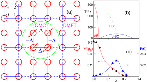
Figure 40: (a) Schematic representation of an antiferromagnetic $d$-wave $2\times 2$ periodically repeated cluster. (b) Generic phase diagram of HTSC. (c) Magnetic (M) and $d$-wave superconducting (F) order parameters versus hole-doping in the 2D Hubbard model at $\beta t=15$, $t^{\prime}=-0.15t$, $U=4.8t$ calculated with a 4-site cluster approach similar to the DCA/QMC. Taken from Lichtenstein and Katsnelson (2000).

In this approach, an $8\times 8$ matrix representation of the Green function is required to account for both the antiferromagnetic order parameter $\langle c^{\dagger}_{i\uparrow}c_{j\downarrow}\rangle$ and the superconducting order parameter $\langle c_{i\downarrow}c_{j\uparrow}\rangle$. Figure 40(c) reproduces the results for the two order parameters as a function of doping at fixed temperature in the weak coupling regime ($U=4.8t$). The authors find that the antiferromagnetic order parameter coexists with the $d$-wave superconducting order parameter over a wide range of doping. Consistent with the DCA/QMC results, the antiferromagnetic order parameter is maximal at zero doping where the superconducting order parameter vanishes due to the opening of the gap.

IV.4.5 Phase diagram

The results reviewed in the preceding sections illustrate that quantum cluster approaches applied to the 2D Hubbard model are able to capture the complex behavior observed in HTSC. The qualitative agreement with experiments is summarized in the $N_{c}=4$ DCA/QMC temperature-doping ($T$-$\delta$) phase diagram of the 2D Hubbard model in the intermediate coupling regime $U=W$ shown in Fig. 41. The phase boundaries were determined by the instabilities of the paramagnetic phase as indicated by the divergence of the corresponding susceptibilities. Therefore these results do not allow any conclusions about a possible coexistence of the antiferromagnetic and $d$-wave superconducting phases for $\delta<0.5$. The results by Lichtenstein and Katsnelson (2000) however suggest this coexistence at least for weak coupling (see Fig. 40(c)).

Figure 41: Temperature-doping phase diagram of the 2D Hubbard model when $U=8t$ calculated with DCA/QMC for a 4-site cluster, $N_{c}=4$. The error bars on $T^{*}$ result from the difficulty in locating the maximum in the uniform spin susceptibility. Regions of antiferromagnetism, $d$-wave superconducting and pseudogap behavior are seen.

The pseudogap crossover temperature $T^{*}$ determined by the peak in the uniform spin susceptibility (see Fig. 32) serves as a boundary separating the observed Fermi liquid and non-Fermi liquid behavior. For $T<T^{*}$ the self-energy shows non-Fermi liquid character for the parts on the Fermi surface near ${\bf{k}}=(\pi,0)$ (see Fig. 34). Quasiparticle and low-energy spin excitations are suppressed as indicated by the pseudogap in the DOS and the spin-susceptibility (see Fig. 38). At $\delta\gtrsim 0.2$ Fermi-liquid behavior is recovered (see Fig. 34). At low temperatures, the systems is antiferromagnetic near half-filling. The $d$-wave superconducting phase at finite doping has its maximum transition temperature at $\delta\approx 0.05$.

As indicated in Sec. IV.4.3, the $N_{c}=4$ DCA cluster favors the spin-charge separated RVB state. The $N_{c}=4$ results may thus be interpreted within the RVB picture Anderson (1987): The pairing of spins in singlets below the crossover temperature $T^{*}$ results in the suppression of low-energy spin excitations and consequently in a pseudogap in the density of states. Charge excitations are quasi-free as indicated by the zero-frequency peak in the charge susceptibility (see Fig. 38). Well below the transition spin and charge degrees of freedom recombine, forming electrons which pair. Frustrated kinetic energy is recovered as indicated by the reduction of the kinetic energy as the system goes superconducting (see Fig. 39).

Although the properties of HTSC are well described by the $N_{c}=4$ results, it is important to ask the question whether the phase diagram and in particular the observed RVB nature of the results are stable when the cluster size is increased. While the pseudogap temperature $T^{*}$ may be expected to persist with increasing $N_{c}$, the transition temperatures to the antiferromagnetic and superconducting state are expected to fall to zero, as discussed in Sec. I.2 (see also Fig. 27). This has been confirmed through simulations of larger clusters Jarrell et al. (2004). A finite inter-planar coupling between an infinite set of Hubbard planes may then be used to stabilize the transitions at larger $N_{c}$, at least to the antiferromagnetic state Jarrell et al. (2001b). The stability of the RVB behavior and even the superconductivity is less clear and more complex models may be necessary for them to persist in larger clusters.

IV.4.6 Studies of related models

Stripes in the t-J-model.

Several numerical studies indicate that there is a tendency for doped holes to form stripes separated by antiferromagnetic domains in strongly correlated systems (for a review see Dagotto, 1994). CPT is the quantum cluster method of choice to study the large unit cells in the inhomogeneous stripe phase, which complicate if not preclude the application of the numerically more expensive embedded cluster techniques (CDMFT, DCA). A thorough study of stripes in the large $U$ limit of the Hubbard model, the t-J model, was conducted by Zacher et al. (2002b, a) within the CPT. To implement the CPT for this problem, the authors divided the lattice into alternating clusters of metallic stripes and antiferromagnetic domains. The inter-cluster hopping linking these clusters was treated perturbatively within the CPT. The enforced stripe pattern in this implementation prohibits to explore the stability of stripes, but allows to investigate the effects of the stripe pattern on the single-particle excitations. In systems with less than 12% doping the technique was shown to reproduce salient ARPES features in selected HTSC if a site-centered 3+1 stripe pattern, i.e. half-filled antiferromagnetic three-leg ladders separated by doped one-leg chains, was chosen Zacher et al. (2002b). At higher dopings the comparison with ARPES indicates that the weight of bond-centered stripes with a 2+2 pattern increases in which excess holes proliferate out of the stripes into the antiferromagnetic domain Zacher et al. (2002a).

Spectral properties of the three-band Hubbard model.

In the context of HTSC, the single-band Hubbard model can be viewed as a low-energy approximation of the more complex and more realistic three-band Hubbard model Emery (1987); Emery and Reiter (1988). The three-band Hubbard model takes into account the $p_{x}$ and $p_{y}$ oxygen orbitals in addition to the Cu $d$ degrees of freedom in the superconducting CuO₂ planes. The CPT study of its spectral properties by Dahnken et al. (2002) shows very good agreement with ARPES data on HTSC at half-filling as well as in the doped system including a hole-like Fermi surface at high doping which splits into an electron- and hole-like branch when a bilayer hopping $t_{\perp}$ is included.

Cluster simulations of the periodic Anderson model.

The periodic Anderson model (PAM) is widely considered to be a paradigm for a variety of rare-earth and actinide compounds including the heavy Fermion systems. It is composed of a strongly hybridizing band of $d$ electrons and a weakly hybridizing band of correlated $f$-electrons described by the Hamiltonian

$$H = -t\sum_{ij,\sigma}(d^{\dagger}_{i\sigma}d_{j\sigma}+h.c.)+\sum_{i}\epsilon_{d}(n^{d}_{i\uparrow}+n^{d}_{i\downarrow})$$ (189)

$$+ \sum_{i}\epsilon_{f}(n^{f}_{i\uparrow}+n^{f}_{i\downarrow})+U\sum_{i}n^{f}_{i\uparrow}n^{f}_{\downarrow}$$

DMFT simulations of the PAM reveal an antiferromagnetic insulating phase at half filling of both the $f$ and $d$ bands. The gap is set by the Kondo coherence scale $T_{0}$ which is strongly enhanced compared to the single-impurity model (SIAM) scale. When the $d$-band is doped away from half filling while the $f$-band remains roughly half filled, the system becomes more metallic, and the Kondo scale is strongly suppressed compared to that of the SIAM. In both the insulator and metal, the temperature dependence of the impurity susceptibility and many other low temperature quantities deviate strongly from that of the SIAM Tahvildar-Zadeh et al. (1997).

Non-local corrections were studied by Shimizu (2002) who used the DCA together with the NCA as a cluster solver to study the single-particle spectra. He finds large deviations from the DMFT result due to the effects of RKKY exchange. At half filling, where the RKKY exchange is strong and antiferromagnetic, he finds a large gap of the order of the RKKY exchange energy. When the filling of the conduction band is small and the RKKY exchange is weaker and ferromagnetic, the coherence peak is restored.

V Conclusions and perspectives

In this review we tried to convey the message that quantum cluster approaches provide powerful theoretical tools to study the rich phenomenology in systems dominated by strong electronic interactions, such as most notably transition metal oxides, heavy Fermion and one-dimensional systems including superconducting and magnetic compounds. Quantum cluster approaches are non-perturbative in nature, their quality can be systematically improved by increasing the cluster size, and they provide complementary information to finite size simulations. By mapping the lattice problem to a finite size cluster they describe short-ranged correlations within the cluster accurately while approximating longer-ranged physics on the mean-field level. Of the various attempts to add non-local corrections to local approximations such as DMFT, we focused in this review on three established quantum cluster approaches which we believe to play the major role in the description of many-particle systems.

The cluster perturbation theory provides a very economic way to calculate the single-particle dynamics by continuing the results of an isolated finite size cluster to the thermodynamic limit. For a cluster consisting of a single site only this method is identical to the Hubbard-I approximation, while it recovers the exact result in the infinite size cluster limit. When combined with the self-energy functional approach, the CPT can also be used to study instabilities to symmetry broken phases.

Both embedded cluster techniques, the dynamical cluster approximation and the cellular dynamical mean field theory are superior to the CPT in that they map the lattice to an embedded cluster instead of the CPT’s isolated cluster. This leads to a self-consistent theory with a single-particle coupling between the cluster and the host. As a result both DCA and CDMFT naturally allow for the study of phase-transitions and they provide thermodynamically consistent results on the one- and two-particle level.

CDMFT can be viewed as a direct generalization of DMFT to a cluster in real space. The mapping between lattice and cluster problems is identical to that of the long established MCPA for disordered systems. It leads to a cluster with open boundary conditions which violates translational symmetries. In contrast the DCA cluster is defined in cluster reciprocal space. Hence the DCA cluster has periodic boundary conditions and therefore preserves the translational symmetries of the lattice. This difference in boundary conditions translates directly to different asymptotic behaviors for large linear cluster sizes $L_{c}$, and the decision which method to use for a given problem strongly depends on the quantities of interest: Local quantities, such as the local density of states when defined on central cluster sites converge faster in the CDMFT since they do not directly couple to the mean-field. Due to the large mean-field coupling of the surface sites however, the CDMFT converges slowly, with corrections of order ${\cal O}(1/L_{c})$, for quantities extended over the cluster. The DCA converges more quickly, as ${\cal O}(1/L_{c}^{2})$, due to the periodic boundary conditions on the cluster.

Quantum cluster approaches reduce the complexity of the infinite lattice problem by mapping it to a cluster with fewer degrees of freedom. The numerous methods employed to solve the DMFT equations are in principle available to study the effective cluster model. However as the complexity of this task rapidly increases with cluster size, potential cluster solvers are faced with severe size limitations. As the most promising techniques we reviewed perturbative approaches including the fluctuation-exchange approximation and the non-crossing approximation as well as non-perturbative techniques including quantum Monte Carlo and numerical renormalization group.

We discussed the application of quantum cluster approaches to a wide range of problems in condensed matter physics. The information gained from these studies has led to significant progress in the field of strongly correlated electron systems. Even studies using small cluster sizes opened up new insight in problems such as one-dimensional systems, the Mott-Hubbard transition in two dimensions and high-temperature superconductivity.

To gain conclusive evidence however, larger cluster size studies are inevitable to verify the information obtained from small clusters. This task is severely hampered by the rapidly increasing complexity with cluster size. Future progress therefore is closely linked to improvements in the efficiency and flexibility of the techniques used to solve the effective cluster problem. Within quantum cluster approaches we explore a coarse-graining approximation in $k$-space. To further reduce the complexity, the same idea could be transfered to the frequency domain. By coarse-graining the frequency dependence of irreducible quantities, correlations on long time scales are neglected, while the short time scale behavior is described accurately. An important aspect in this context is again the causality question. First test results are encouraging; they show that coarse-graining in Matsubara space leads to acausalities, while coarse-graining the real frequency axis does not face this problem Aryanpour et al. (2003a).

Another route to defeat the cluster size problem is to develop hybrid algorithms that treat different length-scales in the problem with different accuracy. As a promising step in this direction, Hague et al. (2003) have developed a hybrid technique which maps the infinite lattice onto two embedded clusters of different size, thus dividing the problem into three length-scales. Short-ranged correlations described by the small cluster are treated accurately within QMC, correlations of intermediate length-scale are treated perturbatively in the large cluster using FLEX, and the long-ranged physics beyond the size of the larger cluster is again approximated on the mean-field level.

To improve comparisons with experiments and to achieve predictive capability, the inclusion of the specifics of the actual materials is required. Along the lines of the LDA+DMFT approach, one can use electronic structure calculations to parameterize the models studied by quantum cluster approaches. First steps in this direction have been made by Poteryaev et al. (2003). A more integrated approach to the ab-initio description of strongly correlated systems by combining the ideas of density functional theory and quantum cluster approaches remains an important and challenging task.

References

- Abrikosov et al. (1963) Abrikosov, A., L. Gorkov, and I. Dzyaloshinski, 1963, Methods of Quantum Field Theory in Statistical Physics (Dover).
- Aichhorn et al. (2003) Aichhorn, M., M. Daghofer, H. Evertz, and W. v.d. Linden, 2003, Phys. Rev. B 67, 161103.
- Anderson (1961) Anderson, P., 1961, Phys. Rev. 124, 41.
- Anderson (1997a) Anderson, P., 1997a, Adv. Phys. 46, 3.
- Anderson (1987) Anderson, P. W., 1987, Science 235, 1196.
- Anderson (1997b) Anderson, P. W., 1997b, The Theory of Superconductivity in the High- Cuprates (Princeton University Press, Princeton, NJ).
- Aryanpour et al. (2002) Aryanpour, K., M. H. Hettler, and M. Jarrell, 2002, Phys. Rev. B 65, 153102.
- Aryanpour et al. (2003a) Aryanpour, K., M. H. Hettler, and M. Jarrell, 2003a, Phys. Rev. B 67, 085101.
- Aryanpour et al. (2003b) Aryanpour, K., T. A. Maier, and M. Jarrell, 2003b, preprint cond-mat/0301460 .
- Baym (1962) Baym, G., 1962, Phys. Rev. 127, 1391.
- Baym and Kadanoff (1961) Baym, G., and L. Kadanoff, 1961, Phys. Rev. 124, 287.
- Becker and Keller (1987) Becker, K., and J. Keller, 1987, Z. Phys. B 36, 2036.
- Beeby and Edwards (1962) Beeby, J. L., and S. F. Edwards, 1962, Proc. Roy. Soc. (London) A274, 395.
- Bethe (1935) Bethe, H. A., 1935, Proc. R. Soc. London A150, 552.
- Betts and Stewart (1997) Betts, D., and G. Stewart, 1997, Can. J. Phys. 75, 47.
- Bickers (1987) Bickers, N., 1987, Rev. Mod. Phys. 59, 845.
- Bickers et al. (1987) Bickers, N., D. Cox, and J. Wilkins, 1987, Phys. Rev. B 36, 2036.
- Bickers et al. (1989) Bickers, N., D. Scalapino, and S. White, 1989, Phys. Rev. Lett. 62, 961.
- Bickers and White (1990) Bickers, N., and S. R. White, 1990, Phys. Rev. B 43, 8044.
- Biroli and Kotliar (2002) Biroli, G., and G. Kotliar, 2002, Phys. Rev. B 65, 155112.
- Biroli et al. (2003) Biroli, G., O. Parcollet, and G. Kotliar, 2003, preprint con-mat/0307587 .
- Bolech et al. (2003) Bolech, C., S. Kancharla, and G. Kotliar, 2003, Phys. Rev. B 67, 075110.
- Brandt and Mielsch (1989) Brandt, U., and U. Mielsch, 1989, Z. Phys. B 75, 365.
- Brandt and Schmidt (1986) Brandt, U., and R. Schmidt, 1986, Z. Phys. B 63, 45.
- Brandt and Schmidt (1987) Brandt, U., and R. Schmidt, 1987, Z. Phys. B 67, 43.
- Bulla (1999) Bulla, R., 1999, Phys. Rev. Lett. 83, 136.
- Bulla et al. (2001) Bulla, R., T. Costi, and D. Vollhardt, 2001, Phys. Rev. B 64, 045103.
- Bulla et al. (1998) Bulla, R., A. Hewson, and T. Pruschke, 1998, J. Phys.: Condens. Matter 10, 8365.
- Caffarel and Krauth (1994) Caffarel, M., and W. Krauth, 1994, Phys. Rev. Lett. 72, 1545.
- Cox and Grewe (1987) Cox, D., and N. Grewe, 1987, Z. Phys. B 71, 321.
- Creffield et al. (1995) Creffield, C., E. Klepfish, E. Pike, and S. Sarkar, 1995, Phys. Rev. Lett. 75, 517.
- Dagotto (1994) Dagotto, E., 1994, Rev. Mod. Phys 66, 763.
- Dagotto and Moreo (1988) Dagotto, E., and A. Moreo, 1988, Phys. Rev. B 38, 5078.
- Dahnken et al. (2003) Dahnken, C., M. Aichhorn, W. Hanke, E. Arrigoni, and M. Potthoff, 2003, preprint cond-mat/0309407 .
- Dahnken et al. (2002) Dahnken, C., E. Arrigoni, and W. Hanke, 2002, J. Low Temp. Phys. 126, 949.
- Deisz et al. (1996) Deisz, J., D. Hess, and J. Serene, 1996, Phys. Rev. Lett. 76, 1312.
- Deisz et al. (2003) Deisz, J., D. Hess, and J. Serene, 2003, Recent Progress in many Body Theories, volume 4 (Plenum, New York).
- Ducastelle (1974) Ducastelle, F., 1974, J. Phys C 7, 1795.
- Emery (1987) Emery, V., 1987, Phys. Rev. Lett. 58, 2794.
- Emery and Reiter (1988) Emery, V., and G. Reiter, 1988, Phys. Rev. B 38, 4547.
- Fetter and Walecka (1971) Fetter, A., and J. Walecka, 1971, Quantum Theory of Many-Particle Systems, International Series in Pure and Applied Physics (McGraw-Hill, New York).
- Fischer (1997) Fischer, K., 1997, Phys. Rev. B 55, 13575.
- Fisher and Barber (1972) Fisher, M., and M. Barber, 1972, Phys. Rev. Lett. 28, 1516.
- Georges and Kotliar (1992) Georges, A., and G. Kotliar, 1992, Phys. Rev. B 45, 6479.
- Georges et al. (1996) Georges, A., G. Kotliar, W. Krauth, and M. Rozenberg, 1996, Rev. Mod. Phys. 68, 13.
- Goldenfeld (1992) Goldenfeld, N., 1992, Lectures on Phase Transitions and the Renormalization Group, Frontiers in Physics (Addison Wesley, Reading, Massachusetts).
- Gonis (1992) Gonis, A., 1992, Green Functions for Ordered and Disordered Systems, Studies in Mathematical Physics (North-Holland, Amsterdam).
- Grewe (1983) Grewe, N., 1983, Z. Phys. B 53, 271.
- Grewe (1987) Grewe, N., 1987, Z. Phys. B 67, 323.
- Grewe et al. (1988) Grewe, N., H. Keiter, and T. Pruschke, 1988, Z. Phys. B 71, 75.
- Gros and Valenti (1994) Gros, C., and R. Valenti, 1994, Annalen der Phys. 3, 460.
- Hague (2003) Hague, J., 2003, J. Phys.: Cond. Mat. 15, 2535.
- Hague et al. (2003) Hague, J., M. Jarrell, and T. Schulthess, 2003, preprint cond-mat/0312155 .
- Haydock et al. (1975) Haydock, R., V. Heine, and M. J. Kelly, 1975, J. Phys. C 8, 2591.
- Heindl et al. (2000) Heindl, W., T. Pruschke, and J. Keller, 2000, J. Phys.: Condens. Matter 12, 2245.
- Hettler et al. (2000) Hettler, M. H., M. Mukherjee, M. Jarrell, and H. R. Krishnamurthy, 2000, Phys. Rev. B 61, 12739.
- Hettler et al. (1998) Hettler, M. H., A. N. Tahvildar-Zadeh, M. Jarrell, T. Pruschke, and H. R. Krishnamurthy, 1998, Phys. Rev. B 58, R7475.
- Hewson (1993) Hewson, A., 1993, The Kondo Problem to Heavy Fermions, Cambridge Studies in Magnetism (Cambridge UNiversity Press, Cambridge).
- Hirsch (1983) Hirsch, J., 1983, Phys. Rev. B 28, 4059.
- Hirsch and Fye (1986) Hirsch, J., and R. Fye, 1986, Phys. Rev. Lett. 56, 2521.
- Hohenadler et al. (2003) Hohenadler, M., M. Aichhorn, and W. v.d. Linden, 2003, Phys. Rev. B 68, 184304.
- Hubbard (1963) Hubbard, J., 1963, Proc. Royal. Soc. London 276, 238.
- Huscroft et al. (2000) Huscroft, C., R. Gass, and M. Jarrell, 2000, Phys. Rev. B 61, 9300.
- Huscroft et al. (2001) Huscroft, C., M. Jarrell, T. Maier, S. Moukouri, and A. Tahvildarzadeh, 2001, Phys. Rev. Lett. 86, 139.
- Imai and Kawakami (2002) Imai, Y., and N. Kawakami, 2002, Phys. Rev. B 65, 233103.
- Itzykson and Drouffe (1989) Itzykson, C., and J.-M. Drouffe, 1989, Statistical Field Theory (Cambridge University Press).
- Jaklič and Prelovšek (2000) Jaklič, J., and P. Prelovšek, 2000, Adv. Phys. 49, 1.
- Jarrell (1992) Jarrell, M., 1992, Phys. Rev. Lett. 69, 168.
- Jarrell et al. (1993) Jarrell, M., H. Akhlaghpour, and T. Pruschke, 1993, Quantum Monte Carlo Methods in Condensed Matter Physics (Worl Scientific, Singapore), chapter Quantum Monte Carlo in the Infinite Dimensional Limit, pp. 221–234.
- Jarrell and Gubernatis (1996) Jarrell, M., and J. Gubernatis, 1996, Physics Reports 269, 133.
- Jarrell and Johnson (2004) Jarrell, M., and D. Johnson, 2004, in preparation .
- Jarrell and Krishnamurthy (2001) Jarrell, M., and H. R. Krishnamurthy, 2001, Phys. Rev. B 63, 125102.
- Jarrell et al. (2001a) Jarrell, M., T. Maier, M. H. Hettler, and A. N. Tahvildarzadeh, 2001a, Europhys. Lett. 56, 563.
- Jarrell et al. (2001b) Jarrell, M., T. Maier, C. Huscroft, and S. Moukouri, 2001b, Phys. Rev. B 64, 195130.
- Jarrell et al. (2004) Jarrell, M., T. Maier, and T. Schulthess, 2004, in preparation .
- Jarrell and Pruschke (1993) Jarrell, M., and T. Pruschke, 1993, Z. Phys. B 90, 187.
- Jones and Varma (1987) Jones, B., and C. Varma, 1987, Phys. Rev. Lett. 58, 843.
- Jones et al. (1988) Jones, B., C. Varma, and J. Wilkins, 1988, Phys. Rev. Lett. 61, 125.
- Kakehashi (2002) Kakehashi, Y., 2002, Phys. Rev. B 66, 104428.
- Kampf and Schrieffer (1990) Kampf, A., and J. Schrieffer, 1990, Phys. Rev. B 42, 7967.
- Keiter and Czycholl (1983) Keiter, H., and C. Czycholl, 1983, J. Magn. and Magn. Mat. 31–34, 477.
- Keiter and Kimball (1970) Keiter, H., and J. Kimball, 1970, Phys. Rev. Lett. 25, 672.
- Keiter and Kimball (1971) Keiter, H., and J. Kimball, 1971, Int. J. Magn. 1, 233.
- Kikuchi (1951) Kikuchi, R., 1951, Phys. Rev. 81, 988.
- Kim et al. (1990) Kim, C., Y. Kuramoto, and T. Kasoya, 1990, J. Phys. Soc. Jpn. 59, 2414.
- Kotliar et al. (2001) Kotliar, G., S. Savrasov, G. Pallson, and G. Biroli, 2001, Phys. Rev. Lett. 87, 186401.
- Krishnamurthy et al. (1980a) Krishnamurthy, H., J. Wilkins, and K. Wilson, 1980a, Phys. Rev. B 21, 1003.
- Krishnamurthy et al. (1980b) Krishnamurthy, H., J. Wilkins, and K. Wilson, 1980b, Phys. Rev. B 21, 1044.
- Kuramoto (1983) Kuramoto, Y., 1983, Z. Phys. B 53, 37.
- Kuramoto (1985) Kuramoto, Y., 1985, Springer Series in Sol. State , 152.