Elastic contact to a coated half-space - Effective elastic modulus and real penetration

Abstract

A new approach to the contact to coated elastic materials is presented. A relatively simple numerical algorithm based on an exact integral formulation of the elastic contact of an axisymmetric indenter to a coated substrate is detailed. It provides contact force and penetration as a function of the contact radius. Computations were carried out for substrate to layer moduli ratios ranging from $10^{-2}$ to $10^{2}$ and various indenter shapes. Computed equivalent moduli showed good agreement with the Gao model for mismatch ratios ranging from 0.5 to 2. Beyond this range, substantial effects of inhomogeneous strain distribution are evidenced. An empirical function is proposed to fit the equivalent modulus. More importantly, if the indenter is not flat-ended, the simple relation between contact radius and penetration valid for homogeneous substrates breaks down. If neglected, this phenomenon leads to significant errors in the evaluation of the contact radius in depth-sensing indentation on coated substrates with large elastic modulus mismatch.

I Introduction

With the increasing use of coated and multilayered systems, there is a growing need for accurate measurement of the mechanical properties of thin films. Amongst the few possible techniques, nanoindentation appears as the most promising. However, the methods used to analyze indentation data (the most commonly used being that by Oliver and Pharr¹) are based on models valid for isotropic homogeneous elastic solids^2,3. As a consequence, the so-called “equivalent elastic modulus”, $E_{\rm eq}$, obtained through these methods is a combination of the respective moduli of the film, $E_{\rm film}$, and of the substrate, $E_{\rm substrate}$. The relative weight of each material, as was pointed out by Doerner and Nix⁴, varies with the penetration depth.

Several models have been proposed to extract intrinsic material properties of the film from this depth-dependent equivalent modulus. Most of them are empirical models based on the following structure:

$$E_{\rm eq}=E_{\rm substrate}+(E_{\rm film}-E_{\rm substrate})\,\Phi(x)$$ (1)

in which $x$ is the ratio of the contact radius, $a$, or the contact depth, $h_{c}$, to the film thickness, $t$, and $\Phi$ is the “weight function” which equals 1 when $x$ is 0 and 0 when $x$ is infinite. The most commonly-used of these models have been summarized and studied experimentally by Men$\breve{c}$ik et al.⁵.

Analytical approaches have also been proposed. The method introduced by Gao et al.⁶ is based on a perturbative calculation of the elastic energy of a coated substrate indented with a flat punch. This approach is based on the assumption that the mechanical properties of both materials do not differ widely. Comparisons with finite-element (FE) calculations proved that this model provides a precise account for load/displacement responses, at least for modulus ratios up to 2. Another approximate approach by Yoffe⁷ focuses on the calculation of an additional stress field which would compensate the inhomogeneity of the coated solid during its indentation by a rigid flat punch. From the latter, an approximate formula linking the global compliance to the geometry of the system is deduced. A third approach, allowing the analytically exact calculation of the stress field in the whole coated material, has been proposed by Schwarzer⁸. Based on results by Fabrikant⁹, it uses an electrostatic-like method of images approach, leading to the calculation of the sum of an infinite series.

In the present work, we propose an alternative method relying on a previous work by Li and Chou¹⁰, in which they calculated the Green function for a coated substrate. Unfortunately, their stress/strain relation could not be inverted, thus proving of little use for contact problems. Using the auxiliary fields introduced by Sneddon^3,11 and later on developed by Huguet and Barthel¹² and Haiat and Barthel¹³, we first reformulated their expression to allow the problem to be inverted at low numerical cost.This approach is developed in Part I.

In Part II, we present the results of our calculations. We first compare our results for the equivalent modulus with the Gao model. Following that, we propose a new fitting function for the contact radius dependence of the equivalent modulus.

As a result for sphere and cone indentation, a non-trivial penetration/contact radius relation is obtained, which differs markedly from the Hertz equation. The implications of these results for data treatment in depth-sensing indentation methods to determine the modulus of very thin films are discussed.

Part I Algorithm

II Green function of a coated substrate

Let us consider a mechanical system composed of a coated elastic half-space under an axisymmetric frictionless loading (Fig. 1). The layer, of thickness $t$, and the half-space are supposed elastic, isotropic and homogeneous, while their adhesion is supposed to be perfect. Let $E_{0}$ and $\nu_{0}$ (resp. $E_{1}$ and $\nu_{1}$) be the elastic modulus and the Poisson ratio of the half-space (resp. of the layer).

Using Hankel transforms, in the framework of linear elasticity, Li and Chou¹⁰ obtained a relation between the applied normal stress $q(r)$ at the surface of the layer (taken positive when compressive) and the normal displacement $u(r)$ (being positive when inwards) in the whole system. Particularizing this general relation between $q$ and $u$ for the surface plane (i.e. for $z=0$), they obtained the following expression:

$$u(r)={{\int_{0}}^{\infty}}dk\,{\overline{q}}(k)J_{0}(kr)\mathcal{C}(kt)$$ (2)

in which we have :

$$\mathcal{C}(kt)={\frac{2}{{E_{1}^{*}}}}{\frac{1+4b\,kt\,{e}^{-2kt}-ab\,{e}^{-4kt}}{1-(a+b+4b{(kt)}^{2}){e}^{-2kt}+ab\,{e}^{-4kt}}}$$

$a={\frac{\alpha\gamma_{3}-\gamma_{1}}{1+\alpha\gamma_{3}}}$, $b={\frac{\alpha-1}{\alpha+\gamma_{1}}}$, $\alpha={\frac{E_{1}(1+\nu_{0})}{E_{0}(1+\nu_{1})}}$, $\gamma_{1}=3-4{\nu}_{1}$ and $\gamma_{3}=3-4{\nu}_{0}$

${E_{1}^{*}}$ being the reduced modulus of the layer defined as $E_{1}/(1-{\nu_{1}}^{2})$, $J_{0}(x)$ the 0^th-order Bessel function of the first kind and ${\overline{q}}$ the 0^th-order Hankel transform of $q$ defined as:

$${\overline{q}}(k)={{\int_{0}}^{\infty}}dr\,r\,J_{0}(kr)\,q(r)$$

Knowing the loading on the whole surface of the system, one may calculate exactly the complete surface displacement. Unfortunately, indentation problems are characterized by mixed boundary conditions : one only knows the surface displacement under the contact and the applied stress outside of it. Thus, Eq. (2), though analytically exact, is of little use in this form. In the following, we propose a reformulation of this expression, which, using auxiliary fields, allows us to bypass this difficulty.

III Introducing auxiliary fields

In order to present a model for the adhesive contact of viscoelastic spheres, Barthel and Haiat¹³ introduced the auxiliary fields $g$ and $\theta$ defined as the following cosine Fourier transforms of the Hankel transforms of the normal surface stress $q(r)$ and displacement $u(r)$ respectively :

$$g(s)={{\int_{0}}^{\infty}}dk\,{\overline{q}}(k)\cos(ks)$$ (3)

$$\theta(s)={{\int_{0}}^{\infty}}dk\,k{\overline{u}}(k)\cos(ks)$$ (4)

Let us first rewrite Eq. (2) with the Hankel transform. We obtain :

$$k{\overline{u}}(k)=\mathcal{C}(kt){\overline{q}}(k)$$ (5)

Let us now apply the cosine Fourier transform to Eq. (5). After some rewriting, we get the following expression :

$$\theta(s)={\frac{2}{\pi}}{{\int_{0}}^{\infty}}g(r)\left({{\int_{0}}^{\infty}}dk\,\mathcal{C}(kt)\cos(kr)\cos(ks)\right)dr$$ (6)

A few comments on Eq. (5) and Eq. (6) are now in order.

IV General comments on the equations

First, we notice that, when turning the system into an homogeneous one, either using the same material for the layer and the substrate or making $t$ nil or infinite, Eq. (5) and Eq. (6) turn into :

$$k{\overline{u}}(k)={\frac{2}{E^{*}}}{\overline{q}}(k)$$ (7)

$$\theta(r)={\frac{2}{E^{*}}}g(r)$$ (8)

These are the equations given by Huguet and Barthel¹² in the case of an homogeneous half-space. The interesting point is that the relation between $\theta$ and $g$ is local (i.e. diagonal), in contrast to Eq. (6). Inversion is therefore straightforward.

Moreover, expressing Eq. (3) and Eq. (4) in the real space, we obtain :

$$g(s)={{\int_{s}}^{\infty}}dr{\frac{rq(r)}{\sqrt{{r}^{2}-{s}^{2}}}}$$ (9)

$$\theta(s)={\frac{d}{ds}}{{\int_{0}}^{s}}dr{\frac{ru(r)}{\sqrt{{s}^{2}-{r}^{2}}}}$$ (10)

Considering the integration limits, one notices that $g$ (resp. $\theta$) depends on $q(r)$ (resp. $u(r)$) only for $r\geq s$ (resp. $r\leq s$). Thus, $g$ and $\theta$ appear to be well-suited to contact problems.

In the case of an homogeneous material, a combination of Eq. (8), Eq. (9) and Eq. (10) allows to solve the problem easily.

In principle, similar auxiliary functions can be built to diagonalize Eq. (6) for the coated system. In practice, as explicit expressions have not been obtained yet, we introduced a numerical method to invert Eq. (6).

V A stress/displacement relation for indentation of a coated solid by a rigid indenter

V.1 Problem definition

Let us now consider Eq. (6) for application to an indentation experiment. Let us not make any hypothesis on the shape of the indenter, apart from the fact that it is rigid, convex, axisymmetric and frictionless. For simplicity, we will consider the contact between the indenter and the coated material to be non-adhesive.

The boundary conditions of this problem are the following :

$$\left\{\begin{array}[]{rl}\displaystyle\forall r\leq a,&u(r)=\delta-h(r)\\ \displaystyle\forall r\geq a,&q(r)=0\end{array}\right.$$ (11)

where $h(r)$ the shape of the indenter and $a$ the contact radius.

Note that this type of loading, because it only considers the normal displacement, does not model the indenter shape exactly, as has been shown by Hay et al.¹⁴. The minor corrections taking into account the radial displacement will not be considered here.

Combining Eq. (9) and Eq. (11), we have :

$$\forall\,r\geq a,g(r)=0$$ (12)

Eq. (6) then becomes :

$$\theta(s)={\frac{2}{\pi}}{{\int_{0}}^{a}}g(r)\left({{\int_{0}}^{\infty}}dk\,\mathcal{C}(k)\cos(kr)\cos(ks)\right)dr$$ (13)

while $\theta(r)$ is known on $[0;a]$ through Eq. (10) and Eq. (11).

Then, under the contact, our indentation problem turns into an integral equation of the type $h(r)={{\int_{0}}^{a}}dsf(s)K(r,s)$ where $h$ and $K$ are known.

As the method is similar whatever the indenter shape, we will only detail here the calculation in the case of the cone indentation, while the case of the flat punch and of the sphere will be developed in appendix A.

V.2 Cone indentation

Under the contact, the given normal surface displacement is $u(r)=\delta-r/\tan(\omega)$, where $\omega$ is the half-included angle of the cone. We deduce that :

$$\forall\,s\leq a,\,\theta(s)=\delta-{\frac{\pi s}{2\tan(\omega)}}$$ (14)

Let us now normalize the contact variable. The appropriate characteristic length in the case of a homogeneous substrate is $a$, as appears in the Hertz theory. When turning an homogeneous substrate into a coated one, we introduce another characteristic scale which is the layer thickness $t$. Thus, we expect an appropriate normalization to exhibit the ratio $a/t$. Indeed, one notes that ${ta^{2}}/{a^{3}}$ is an estimate of the fraction of the “elastically active volume” in the film. Normalizing the length by $a$ also normalizes all the other quantities by the values obtained for the homogeneous material with the mechanical characteristics of the layer.

If we now introduce the function $\mathcal{Z}$, defined as follows, $\mathcal{Z}(x)={\frac{E_{1}^{*}}{2}}\mathcal{C}(x)-1$, we obtain :

$$\theta(s)={\frac{2}{E_{1}^{*}}}g(s)+{\frac{2}{\pi}}{{\int_{0}}^{a}}g(r)\left({{\int_{0}}^{\infty}}dk\,{\frac{2}{E_{1}^{*}}}\mathcal{Z}(kt)\cos(kr)\cos(ks)\right)dr$$ (15)

This expresses the global response of the system to mechanical stress as the reaction of a semi-infinite film to which is added a corrective term quantifying the substrate effect. This expression is similar to the approach of the problem by Yoffe⁷ in the specific case of a flat punch indentation of a coated material.

We then introduce the following normalized quantities :

$$\rho\equiv{\frac{r}{a}};\,\varsigma\equiv{\frac{s}{a}};\,\tau\equiv{\frac{t}{a}};\,\eta\equiv ka$$ (16)

$$\Delta\equiv{\frac{2\delta\tan(\omega)}{\pi a}}$$ (17)

$$\mathcal{Z}(x)\equiv{\frac{E_{1}^{*}}{2}}\mathcal{C}(x)-1$$ (18)

$$G(r)\equiv{\frac{4\tan(\omega)g(r)}{\pi a{E_{1}^{*}}}}$$ (19)

Then Eq. (13) reads :

$$\forall\,\varsigma\leq 1,\,\Delta-{\varsigma}=G(\varsigma)+{\frac{2}{\pi}}{{\int_{0}}^{1}}G(\rho)\left({{\int_{0}}^{\infty}}d\eta\,\mathcal{Z}(\eta\tau)\cos(\eta\rho)\cos(\eta\varsigma)\right)d\rho$$ (20)

The normalized applied force is :

$$\Pi={\frac{4\tan(\omega)}{\pi a^{2}E_{1}^{*}}}P=4{{\int_{0}}^{1}}d\rho\,G(\rho)$$ (21)

And the normalized equivalent modulus is :

$${\mathcal{E}}_{\rm eq}^{*}={\frac{E_{\rm eq}^{*}}{E_{1}^{*}}}={\frac{\Pi}{2{\Delta}^{2}}}$$ (22)

VI Numerical treatment of the equations

VI.1 Implementation of the model

Let us consider Eq. (20) and discretize $[0;1]$ into $N$. From now on, we shall use $\varsigma_{i}={{i}/{N}}$ and $\rho_{j}={{j}/{N}}$. If we approximate the integral on $\rho$ by a discrete sum, we then get :

$$\Delta-\varsigma_{i}=G(\varsigma_{i})+{\frac{1}{N\pi}}G(0)K(\varsigma_{i},0,\tau)+{\frac{1}{N\pi}}G(1)K(\varsigma_{i},1,\tau)+{\frac{2}{N\pi}}\sum_{j=1..N-1}G(\rho_{j})K(\varsigma_{i},\rho_{j},\tau)$$ (23)

with $K(\varsigma,\rho,\tau)={{\int_{0}}^{\infty}}d\eta\,\mathcal{Z}(\eta\tau)\cos(\eta\rho)\cos(\eta\varsigma)$

From Eq. (12) we have $G(1)=0$. Then, for a given $\tau$ — that is to say for a given contact radius — we have to solve the $(N+1)\times(N+1)$ linear system introduced in Eq. (23) for the remaining $N$ values of the $G$ field and the normalized penetration $\Delta$. The $\underline{\underline{K}}$-matrix elements can be calculated with a Fast Fourier Transform (FFT) algorithm for numerical efficiency. Finally, the applied load $\Pi$ and equivalent modulus $\mathcal{E^{*}_{\rm eq}}$ are obtained through Eq. (21) and Eq. (22).

VI.2 Numerical considerations

The accuracy of the numerical solution depends on the dimension $N$ of the $\underline{\underline{K}}$ matrix (which is associated to the discretization of $[0;1]$), the cut-off $B$ for the sampling range of the $\mathcal{Z}$ function and the sampling rate $B/2^{k}$ for the FFT calculation of the matrix elements.

As $\mathcal{Z}$ decreases in an exponential-like way and tends to zero when $\eta$ becomes infinite, it is possible to choose a rather small value for $B$. We first considered the case $a/t=100$ and chose $B=1000$. We then tested increasing values of $N$ and $k$. Our results appear to converge with a deviation smaller than 1$\%$ when $N$ is greater than 700 (for a given $k$ of 19) and when $k$ is greater than 14 (with $N$=700).

However, with $N=700$ and $B=1000$, the output returned for small values of $a/t$ converges only for $k=20$, as the decay length of $\mathcal{Z}$ decreases with $a/t$. This leads to an increase in term of calculation time. Thus, we decided to fix $N=700$ and $k=14$, which constitutes a good compromise between calculation time and precision, and to adapt the value for $B$ to the input value for $a/t$. For instance, for $a/t<1$, $B=20$ is sufficient as $\mathcal{Z}(20)/\mathcal{Z}(0)$ is smaller than $10^{-14}$ for moduli ratios up to 100.

Part II Results

In the following we will consider our results for the equivalent modulus, ${\mathcal{E}}_{\rm eq}^{*}$, and the normalized penetration, $\Delta$. The substrate to layer moduli mismatch ratio ($E_{0}^{*}/E_{1}^{*}$) spans the range $10^{-2}$-$10^{2}$.

VII Equivalent modulus

VII.1 The equivalent homogeneous material

For a given penetration $\delta$, let us define the “equivalent homogeneous material” of a coated substrate as the homogeneous material which would need the same applied load $P$ to get the same penetration $\delta$ with the same indenter tip. Obviously, this material would have a modulus equal to the “equivalent modulus” of the coated substrate for the given penetration.

VII.2 Comparison with the Gao model

We computed the equivalent modulus for flat-punch, sphere and cone indentations for several moduli mismatch ratios ranging from $10^{-2}$ to $10^{2}$. The comparison of the three sets of curves shows that the same coated system being indented with different indenter tips (flat-punch, cone or sphere) does not return the same equivalent modulus for a given contact radius. However, the qualitative evolution of the curves with the mismatch ratio ($E_{0}^{*}$/$E_{1}^{*}$) is the same, and sphere and cone indentation curves almost superimpose (Fig. 2).

Thus Fig. 3 only shows the evolution, for several mismatch ratios, of the equivalent modulus with the relative contact radius for cone indentations. Fig. 3(a) details the case of soft films on a stiff substrate, whereas Fig. 3(b) represents the case of stiff layers on a soft substrate. In all cases, the equivalent modulus exhibits a transition from layer to substrate modulus as the contact radius goes from zero to infinity.

One can notice that, whatever the indenter shape, all curves almost have the same shape, regardless of the moduli mismatch between the layer and the substrate. This shape indeed is very much like that provided by Gao et al.⁶. In particular, when the moduli mismatch ratio converges to one, our curves converge to the Gao model (Fig. 4). The agreement is good in the range 0.5-2. When the mismatch is larger, the shape of the $E^{*}_{\rm eq}$ curves is almost unchanged but the transition range, over which the system response changes from one limit behavior to the other, appears to shift from the position given by Gao. When indenting a soft layer on a stiff substrate, the range over which the behavior of the system is close to that of the film increases with the modulus mismatch, whereas it conversely shrinks when indenting stiff layers.

The analytical model introduced by Gao et al.⁶ is based on a perturbative analysis. Thanks to FE calculations, they showed that their model is correct on the range 0.5-2. Thus, the agreement of our results in the same range was to be expected.

As to the shift of the transition range for large modulus mismatch, we note that in their analysis, Gao et al. used the stress and displacement values calculated for an homogeneous material. Thus, their analysis accounts for a homogeneous distribution of the strain in the coated substrate. However, the strain caused by indentation is a priori distributed inhomogeneously in an inhomogeneous system. Indeed, as one of the materials is softer than the other one, it tends to absorb a greater part of the global strain. This means that the softer material always dominates in the compound system response. Thus, when indenting a soft film on a stiff substrate, most of the strain being “confined” in the layer, the transition is shifted towards greater relative contact radii. Conversely, when indenting a stiff layer, it is the substrate which absorbs most of the strain and the transition range is shifted to smaller $a/t$. Naturally, this effect tends to increase with increasing modulus mismatch.

As a result, the curve provided by the Gao model stands as a limit between stiff layers and soft layers in our calculations (Fig. 4(b)). We are now in position to extend empirically the Gao function on a wider range of moduli ratios.

VII.3 Equivalent modulus : Empirical description

As the $({E^{*}_{\rm eq}};a/t)$ curves resulting from our calculations exhibit similar shapes, it appears reasonable to look for a fit function that would expand the Gao function to a larger range of moduli ratios. We propose the following function :

$${{E^{*}_{\rm eq}}}\left({\frac{a}{t}}\right)={{E^{*}_{1}}}+{\frac{({{E^{*}_{0}}}-{{E^{*}_{1}}})}{1+{({\frac{tx_{0}}{a}})}^{n}}}$$

where $x_{0}$ and $n$ are adjustable constants.

The parameter $x_{0}$ is the value of the $a/t$ ratio for which ${{E^{*}_{eq}}}=({E^{*}_{0}}+{E^{*}_{1}})/2$. At the same time it corresponds to the change in curvature of the $({E^{*}_{\rm eq}};a/t)$ curve plotted in semi-log coordinates.

Table I presents the results of our fit for cone contacts. The parameter $x_{0}$ (which characterizes the position of the transition range) increases with moduli mismatch ratio, as was expected. Using our results we obtained the following relation on a wide range of moduli mismatch :

$$\log(x_{0})=-0.093+0.792\log({E_{0}^{*}}/{E_{1}^{*}})+0.05\left(\log({E_{0}^{*}}/{E_{1}^{*}})\right)^{2}$$

On the other hand, $n$ (which characterizes the width of the transition range) does not change much on the $10^{-2}-10^{2}$ range.

VIII The real penetration

The contact is described by three variables: the force, the penetration and the radius of the contact zone, or contact radius. For elastic systems, there exist two relations between these three variables. For homogeneous half-spaces, these are the two well-known relations due to Hertz in the case of a sphere. The first relation links force and penetration. In the case of a coated substrate, this relation leads to the introduction of the effective elastic modulus which we have discussed so far. The second relation links penetration and contact radius. It is as simple as $\delta=\pi a/2\tan\omega$ in the case of a cone. Does this simple result remain unchanged when the substrate is inhomogeneous?

For a coated substrate, we calculated the actual force and penetration as a function of the contact radius. We defined the normalized penetration $\Delta$ as the ratio of the actual penetration, $\delta$, to the equivalent penetration $\delta_{\rm eq}$ that would be obtained for the same given contact radius $a$, with an homogeneous material (See Fig. 5). Thus, when $\Delta$ is close to 1, the coated material behaves as if homogeneous. A behaviour specific to coated substrates is evidenced when $\Delta$ departs from 1.

VIII.1 Evolution of the actual penetration during indentation

$\Delta$ as a function of $a/t$ is plotted on Fig. 6 for cone and sphere indentation. The case of flat-punch indentation is irrelevant here as $a$ is a fixed parameter (Appendix A). Fig. 6(a) shows the evolution of $\Delta$ for the indentation of soft layers, whereas Fig. 6(b) represents the indentation of hard layers. In both graphs, the dashed and marked lines represent the sphere indentations (right scale) while solid lines represent the cone (left scale).

It can be noticed that, for these two indenter shapes, the $(\Delta;a/t)$ curves are similar for a given moduli mismatch. Indeed, one set of curves can be approximately re-scaled on the other by $\Delta^{\rm sphere}-1=\kappa\left(\Delta^{\rm cone}-1\right)$ where the geometrical factor $\kappa$ is around 1.37.

Fig. 6 shows that effects specific to coated materials appear for an intermediate range of $a/t$ values. The width of this range increases with the moduli mismatch. A superposition of Fig. 3 to Fig. 6 provides a simple interpretation of this phenomenon.

Let us consider the case of the indentation of a soft film on a stiff substrate (Fig. 6(a)). The equivalent penetration tallies with the actual penetration for very small relative contact radii because the substrate effect is then just a perturbation, and thus can be neglected in first approximation. Similarly, when the relative contact radius is very large, the system behaves as if there were no film. In the intermediate range, for a given $a$, $\Delta<1$ means that the effective penetration is smaller than the homogeneous equivalent penetration for the same given contact radius $a$. Then, for a given $\delta$, the actual contact radius is greater for the coated substrate than it is for the homogeneous equivalent material. In fact, the applied strain is somehow confined into the layer material, which elastically piles up causing the contact radius $a$ to increase (and so the reduced penetration $\Delta$ to decrease). When the stress applied on the film becomes important enough, the substrate begins to distort substantially, the elastic pile-up is less significant and $\Delta$ increases, until the penetration is so important that the film effect becomes negligible. Then the system turns back to homogeneous substrate behavior. Conversely, for stiff films on soft substrates, a larger penetration at identical contact radius is obtained because of the compliance of the substrate ($\Delta>1$).

Finally, we conclude that, in the case of coated materials, even if a contact radius dependent equivalent modulus can be defined, the $\delta-a$ relation valid for homogeneous systems is no longer systematically observed. This effect, previously described by El-Sherbiney and Halling¹⁵ apparently without much echo, cannot be evidenced in flat punch calculations as $\delta$ is independent from $a$. In fact, to mimic the definition of an equivalent modulus, we would have to introduce a penetration-dependent “equivalent geometrical parameter” equal to the radius (resp. the semi-included angle) of the indenter tip that would give the same $\delta-a$ relation if the system were homogeneous.

A few qualitative considerations can be made on the evolution of this parameter. First, the range of relative radii on which it departs from the actual radius (resp. semi-included angle) corresponds to the transition range previously introduced for the $(E_{\rm eq}^{*};a/t)$ curves (See Fig. 3 and Fig. 6). Secondly, the greater the moduli mismatch, the larger the maximum deviation of the equivalent geometrical parameter from its actual value becomes.

VIII.2 Experimental methods, analytical models and actual penetration

Let us recall two of the basic relations that are used in the Oliver and Pharr depth-sensing indentation method¹ :

$${E}^{*}={\frac{\sqrt{\pi}S}{2\beta\sqrt{A}}}$$ (24)

$$h_{c}=\delta-\varepsilon{\frac{P}{S}}$$ (25)

where $S$ is the contact stiffness, $A$ the contact area, $h_{c}$ the contact depth and $\beta$ and $\varepsilon$ parameters depending on the shape of the indenter tip.

Let us comment on these equations: the discussion deals with the cone, but the case of the sphere is similar. When indenting a real system with a sharp indenter, the core problem to evaluate both elastic and plastic properties is to separate elastic and plastic contributions. Linear superposition shows that Eq. (24) holds for an inhomogeneous substrate, provided ${E}^{*}$ is the flat punch equivalent modulus for the contact radius $a$.

However, in the Oliver-Pharr method, the contact area is derived from $h_{c}$ as calculated with Eq. (25). For an homogeneous substrate, the validity of Eq. (25) stems from the fact that both $\delta$ and $P/S$ are proportional to $a$. This is actually the starting point for the calculation of the value of $\varepsilon$. For a coated substrate, we have shown that $\delta$ is no longer proportional to $a$. Similarly, $P/S$ also deviates from a linear behaviour. Eq. (25) is therefore likely to break down, which we checked in a few sample cases.

Thus, for significant modulus mismatch, the contact radius $a$ calculated from Eq. (25) may be in error by up to 25% for an elastic modulus mismatch of 100 (See Fig. 6(a)). This error will propagate to the effective modulus derived from Eq. (24) and to the layer modulus inferred from the effective modulus.

IX Conclusion

We introduced an analytically exact approach based on the Green function for coated materials calculated by Li and Chou¹⁰. Using a basis of functions well-suited for the mixed boundary conditions, we obtained an integral relation that was easily solved numerically. Based on this relation, we set up an algorithm which provides, given the contact radius, applied force and penetration, for arbitrary moduli ratios and arbitrary axisymmetric indenter shape.

For moduli mismatch ratios close to 1, our results showed good agreement with the Gao model. On a wider range of moduli ratios, we have shown that, for soft layers (resp. stiff layers), the transition from layer to substrate-dominated behavior shifts to larger contact radii (resp. smaller contact radii) with increasing moduli mismatch. We rationalized this results in terms of inhomogeneous strain distribution in the coated material. Based on our computations, we provide an empirical function to describe the (${E^{*}_{\rm eq}}$; $a/t$) curves on a large range of modulus mismatch ratios.

In addition, we have evidenced that, for indention of a coated material with a non-flat indenter, the penetration to contact radius relation significantly deviates from what it is for a homogeneous substrate. This result casts some doubts on the validity of the Oliver and Pharr equations in coated systems mechanical evaluation. On-going work investigates the application of the present method to an Oliver-Pharr-like data treatment for coated material.

ACKNOWLEDGMENTS

The authors would like to acknowledge Stéphane Roux for his help and advice, particularly on the mathematical and numerical aspects of the algorithm.

REFERENCES

1. W. C. Oliver and G. M. Pharr, J. Mater. Res. 7 ,1564 (1992).

2. H. Hertz, J. Reine und angewandte Mathematik 92, 156 (1882).

3. I. N. Sneddon, Fourier Transforms (McGraw-Hill Book Company, Inc., New York, 1951).

4. M. F. Doerner and W. D. Nix, J. Mater. Res 1, 601 (1986).

5. J. Men$\breve{c}$ik, D. Munz, E. Quandt, E. R. Weppelmann and M. V. Swain, J. Mater. Res 12, 2475 (1997).

6. H. J. Gao, C. H. Chiu and J. Lee, Int. J. Solids Structures 29, 2471 (1992).

7. E. H. Yoffe, Ph. Mag. Let 77, 69 (1998).

8. N. Schwarzer, Journal of Tribology 122, 672 (2000).

9. V. I. Fabrikant, Application of Potential Theory in Mechanics : A Selection of New Results (Kluwer Academic Publishers, The Netherlands, 1989).

10. J. Li and T. W. Chou, Int. J. Solids Structures 34, 4463 (1997).

11. I. N. Sneddon, Int. J. Engng. Sci. 3, 47 (1965).

12. A. Huguet and E. Barthel, J. Adhesion 74, 143 (2000).

13. G. Haiat and E. Barthel, Langmuir 18, 9362 (2002).

14. J. C. Hay, A. Bolshakov and G. M. Pharr, J. Mater. Res. 14, 2296 (1999).

15. M. El-Sherbiney and J. Halling, Wear 40, 325 (1976).

CAPTIONS

Fig.1 : Schematic representation of the indentation of a coated elastic half-space.

Fig.2 : Evolution of the equivalent modulus ${E_{\rm eq}}^{*}$ with $a/t$ for flat-punch (dashed), cone (plain) and sphere (markers) indentation for ${E_{0}}^{*}/{E_{1}}^{*}=0.1$($\times$) and ${E_{0}}^{*}/{E_{1}}^{*}=10$($+$). All curves are different but cone and sphere indentation almost coincide.

Fig.3 : Evolution of the equivalent modulus with the moduli mismatch ratio in the case of the indentation by a cone of soft layers (a)($E_{0}^{*}/E_{1}^{*}=2$ ($+$); 5 ($\blacksquare$); 10 ($\blacktriangle$) ; 100 ($\times$)) and stiff layers (b)($E_{0}^{*}/E_{1}^{*}=0.5$ ($+$); 0.2 ($\blacksquare$); 0.1 ($\blacktriangle$) ; 0.01 ($\times$)). The bold dashed line is the Gao function⁶.

Fig.4 : Evolution of the equivalent modulus with the contact radius in the case of moduli mismatch($E_{0}^{*}/E_{1}^{*}$) of 0.5 ($\blacktriangle$), 0.9 ($\times$), 1.1 ($+$) and 2 ($\blacksquare$) for cone indentations (a) and flat punch indentations (b). Our results converge to the Gao model (bold dashed line) when the moduli mismatch tends to 1. Moreover, the transition range for stiff layers (resp. soft layers) is shifted towards smaller (resp. larger) values of $a/t$, in comparison to the transition range given by the Gao model.

Fig.5 : Schematic representation of the indentation of a coated substrate and its equivalent homogeneous material in the case of a soft layer on a stiff substrate ($\Delta<1$). For the same given contact radius, two different penetrations are obtained.

Fig.6 : Evolution of the normalized penetration $\Delta$ in our calculation for soft layers (a)($E_{0}^{*}/E_{1}^{*}=2$ ($+$); 5 ($\blacksquare$); 10 ($\blacktriangle$) ; 100 ($\times$)) and stiff layers (b)($E_{0}^{*}/E_{1}^{*}=2$ ($+$); 5 ($\blacksquare$); 10 ($\blacktriangle$) ; 100 ($\times$)) for sphere (dashed and marked) and cone (solid line) indentations. The same system indented with two different indenters returns curves which can be approximately scaled onto each other by a scaling factor of 1.37.

TABLES

$E_{0}^{*}/E_{1}^{*}$	$x_{0}$	$n$	$E_{0}^{*}/E_{1}^{*}$	$x_{0}$	$n$
100	52.95	1.06	0.67	0.60	1.27
50	25.17	1.09	0.5	0.48	1.27
25	12.55	1.13	0.2	0.24	1.29
10	5.36	1.18	0.1	0.14	1.31
5	2.96	1.22	0.04	0.082	1.32
2	1.41	1.26	0.02	0.052	1.31
1.5	1.13	1.27	0.01	0.032	1.27

Table I : Values obtained for $x_{0}$ and $n$ while fitting the computed equivalent modulus curves for cone indentation (see text).

Appendix A Expressions for other commonly-used indenter shapes

A.1 Flat punch indenter

Let us consider first the case of the flat punch indenter, which is the simplest. As the displacement is constant, using (10) we get :

$$\forall\,s\leq a,\,\theta(s)=\delta$$ (26)

Combining Eq. (13) and Eq. (26), we get :

$$\forall\,s\leq a,\,\delta={\frac{2}{\pi}}{{\int_{0}}^{a}}g(r)\left({{\int_{0}}^{\infty}}dk\,\mathcal{C}(kt)\cos(kr)\cos(ks)\right)dr$$ (27)

With a normalization similar to that introduced for the cone, we get the following normalized quantities :

$$\rho\equiv{\frac{r}{a}}\,;\,\varsigma\equiv{\frac{s}{a}}\,;\,\tau\equiv{\frac{t}{a}}\,;\,\eta\equiv ka$$ (28)

$$\mathcal{Z}(x)\equiv{\frac{E_{1}^{*}}{2}}\mathcal{C}(x)-1$$ (29)

$$G(\rho)\equiv{\frac{2\,g(\rho)}{\delta\,E_{1}^{*}}}$$ (30)

Introducing these quantities in Eq. (27), we get :

$$\forall\,\varsigma\leq 1,\,1=G(\varsigma)+{\frac{2}{\pi}}{{\int_{0}}^{1}}G(\rho)\left({{\int_{0}}^{\infty}}d\eta\,\mathcal{Z}(\eta\tau)\cos(\eta\rho)\cos(\eta\varsigma)\right)d\rho$$ (31)

Through this normalization, we can get the expression of a normalized applied load and a normalized equivalent elastic modulus, thanks to the expression of $G(\rho)$.

$$\Pi=4{{\int_{0}}^{1}}d\rho\,G(\rho)$$ (32)

$${\mathcal{E}}_{\rm eq}^{*}={\frac{E_{\rm eq}^{*}}{E_{1}^{*}}}={\frac{\Pi}{4}}$$ (33)

A.2 Sphere indentation

In the case of a sphere indentation, we have $u(r)=\delta-r^{2}/(2R)$, $R$ being the radius of the sphere. We thus can write, using Eq. (10), that under the contact:

$$\forall\,s\leq a,\,\theta(s)=\delta-{\frac{s^{2}}{R}}$$ (34)

Similarly to the case of the cone, we introduce the following normalized quantities:

$$\rho\equiv{\frac{r}{a}}\,;\,\varsigma\equiv{\frac{s}{a}}\,;\,\tau\equiv{\frac{t}{a}}\,;\,\eta\equiv ka\\$$ (35)

$$\Delta\equiv{\frac{\delta R}{a^{2}}}\\$$ (36)

$$\mathcal{Z}(x)\equiv{\frac{E_{1}^{*}}{2}}\mathcal{C}(x)-1$$ (37)

$$G(r)\equiv{\frac{2R\,g(r)}{a^{2}\,E_{1}^{*}}}$$ (38)

We then get :

$$\forall\,\varsigma\leq 1,\,\Delta-{\varsigma}^{2}=G(\varsigma)+{\frac{2}{\pi}}{{\int_{0}}^{1}}G(\rho)\left({{\int_{0}}^{\infty}}d\eta\,\mathcal{Z}(\eta\tau)\cos(\eta\rho)\cos(\eta\varsigma)\right)d\rho$$ (39)

$$\Pi={\frac{2PR}{a^{3}\,E_{1}^{*}}}=4{{\int_{0}}^{1}}d\rho\,G(\rho)$$ (40)

$${\mathcal{E}}_{\rm eq}^{*}={\frac{E_{\rm eq}^{*}}{E_{1}^{*}}}={\frac{3}{8}}{\frac{\Pi}{{\Delta}^{{3/2}}}}$$ (41)

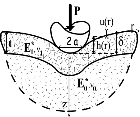
Figure 1:

Figure 2:

Figure 3:

Figure 4:

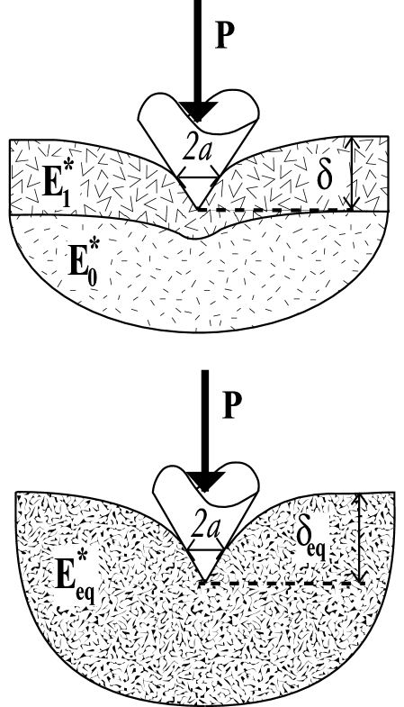
Figure 5:

Figure 6: