Promotiecommissie

Promotor:	Prof. dr. L. J. de Jongh
Referent:	Prof. dr. G. Aeppli (University College London, Groot Britannië)
Overige leden:	Dr. H. B. Brom
	Prof. dr. G. Frossati
	Prof. dr. P. H. Kes
	Prof. dr. M. Orrit
	Prof. dr. J. Zaanen

ISBN: 90-77595-20-1
Printed by Optima Grafische Communicatie, Rotterdam: www.ogc.nl
 
This work is part of the research program of the Stiching voor Fundamenteel Onderzoek der Materie (FOM), which is supported by the Nederlandse Organisatie voor Wetenschappelijk Onderzoek (NWO).

 

Cover: a sequence of nuclear spin echo traces obtained at increasing time intervals after the inversion of the ⁵⁵Mn nuclear polarization in Mn₁₂-ac. The recovery of the equilibrium polarization is driven by quantum tunneling of the cluster spin.

Said the straight man
                                                                     to the late man:
                                                                     “Where have you been?”
                                                                     “I’ve been here and
                                                                     I’ve been there and
                                                                     I’ve been …in between.”

                                                                     King Crimson,
                                                                     “I talk to the wind”, 1969.

Chapter 1 Introduction

Physicists, chemists and biologists have worked since decades on the study of systems of increasing complexity, just as much as engineers and technologists have been trying to miniaturize the devices they design for practical applications. It seems that these two directions have now come very close to a joining point that happens to be located at the nanometer-scale. Accordingly, the name “Nanoscience” has been given to the resulting broad field of research. The rate at which laboratories and research groups are being converted to activities in nanoscience, may raise some fears that it will become a fashion-driven hype. On the other hand, it is undeniable that nanoscience is in fact nothing else than the natural evolution of last century’s science, with a solid history of interests behind it. The subject of this thesis, that could be summarized as the quantum dynamics of magnetic molecules, is a good example of multidisciplinary topic that combines fundamental and practical aspects of the research at the nanometer scale.

The field of molecular magnetism has its roots in the interest of chemists towards the synthesis of large molecules, and the assembly of macroscopic amounts of them in regular structures. Along this route, it became clear that the synthesis of molecules having magnetic ions as constituents could give rise to structures where each molecule can be seen as a single-domain magnetic particle [1], often called “cluster”, coordinated by a shell of organic ligands. Importantly, such molecules are stoichiometric chemical compounds that can be packed in a crystalline structure, where the identical magnetic units interact only weakly with each other. In this way, each molecule can be treated in first approximation as a single nanometer-scale magnet, from where the name “Single Molecule Magnet” (SMM), and is characterized by a large total spin $\vec{S}$ that arises from the combination of the atomic electron spins. The possibility of combining magnetic ions and organic ligands in the most diverse ways allows to tune the physical properties of these systems to obtain a wide range of magnetic behaviors.

One of the most essential physical properties of SMMs is their magnetic anisotropy, meaning that it may be energetically favorable for the magnetic moment of each molecule to align along a certain axis. At temperatures much lower than the anisotropy energy, the molecular spin is effectively “frozen” in a certain direction along the anisotropy axis, giving rise to single-molecule magnetic hysteresis [2]. This discovery in a molecular cluster containing a core of 12 manganese ions (Mn₁₂-ac) opened the perspective of using SMMs as the ultimate magnetic memory units [3].

At the same time, people interested in the fundamental aspects of quantum mechanics at the macroscopic scale (the “Schrödinger cat” problem [4]) realized that SMMs could be candidates for the observation of quantum phenomena at the macromolecular level, in particular quantum tunneling of the magnetic moment [5, 6]. This has been indeed recently achieved by observing regular steps in the magnetic hysteresis loops of Mn₁₂-ac [7, 8], which occur when spin states on opposite sides of the anisotropy barrier have the same energy, so that the cluster spin may invert its direction by resonant quantum tunneling. Again, this discovery is important for both practical and fundamental reasons. On the one hand, it makes clear that a memory unit based on systems as small as a single molecule would be useless if we cannot avoid the memory being self-erased by quantum tunneling. On the other hand, it suggests the possibility of using SMMs as a test ground for theories concerning the transition from quantum to classical physics [9, 10], in particular as far as the role of the environment is concerned.

One of the great advantages of SMMs for fundamental research on quantum mechanics at the large scale is precisely that the influence of the environmental degrees of freedom on the giant molecular spin can be accurately calculated, thanks to the knowledge of the crystal structure and the magnetic couplings between the localized moments. Furthermore, the experimental investigations can profit of all the best known techniques for solid-state physics. Since the pure quantum behavior in SMMs is typically achieved only in the subkelvin temperature range, this research requires the use of outstanding low-temperature facilities for magnetic measurements. In chapter II we describe the working principles and the guidelines for the design of several ultra-low temperature setups that are particularly suitable for experiments on quantum magnetism.

As mentioned above, the magnetic properties of SMMs are determined in the first place at the chemistry level, but an essential aspect is that it is also possible, given a certain SMM, to tune its quantum mechanical behavior “in situ” by applying an external magnetic field. In particular, one can increase the tunneling rate of $\vec{S}$ by applying a field perpendicular to the anisotropy axis of the molecule [11]. This can be pushed to such an extent that we may expect the possibility to observe coherent quantum oscillations of the magnetic moment trough the anisotropy barrier [12], a phenomenon that has no classical analog. In this case, SMMs would become suitable qubits for quantum computing [13], with the interesting feature that the operating frequency can be tuned locally by the simple application of a magnetic field.

A large part of this thesis is dedicated to the study of the interaction between SMMs and their environment, in particular the nuclear spins. This interaction is crucial from many points of view. In the zero- or low-field regime, the tunneling probability is very small, in fact so small that, until recently, there were serious doubts about the observability of quantum tunneling of the magnetic moment in SMMs. This is due the fact that, in order to tunnel, the total electron spin states on opposite sides of the anisotropy barrier must be in resonance within an energy $\Delta$ that can be as small as $\sim 10^{-11}$ K in Mn₁₂-ac. Any static perturbation larger than that, would destroy the resonance condition and make tunneling impossible. Prokof’ev and Stamp [14, 15] succeeded in explaining why tunneling was actually observed in the experiments, by noticing that the coupling of the cluster spin with the nuclear spins in its surroundings, although several order of magnitude larger than $\Delta$, is dynamic. The electron spin energy levels are therefore fluctuating in time with respect to each other, which gives rise to an effective “tunneling window” that depends on the strength of the coupling with the nuclei, as was subsequently demonstrated by experiments with isotopically substituted samples [16]. In the opposite regime, where the fast quantum oscillations of $\vec{S}$ can be obtained by applying a strong perpendicular field, the nuclear spins play the role of an intrinsic source of decoherence. Understanding this phenomenon is obviously essential for any attempt to use a magnetic qubit for quantum computing, since nuclear spins are an unavoidable presence in practically any material. The decoherence due to nuclear spins is indeed important also for systems like the flux qubit [17]. Chapter III of this thesis is dedicated to a review of the theoretical aspects of the quantum behavior of SMMs, from the basic notions to the details of the Prokof’ev-Stamp theory.

Despite its relevance, the nuclear spin dynamics in SMMs at ultra-low temperature remained an essentially unexplored field. In chapter IV we report a thorough investigation of the dynamics of ⁵⁵Mn nuclei in Mn₁₂-ac. Our results uncover many basic aspects, some of which confirm the validity of the Prokof’ev-Stamp theory, while others are totally new and have never been considered in any theoretical treatment of the coupled system of “quantum spin + nuclei”. For instance, we demonstrate that the quantum tunneling of the electron spin is a mechanism capable of producing nuclear relaxation at an unexpectedly high rate. We also show that nuclei in different molecules are coupled with each other, an essential ingredient for the creation of a dynamic tunneling window. The analysis of the nuclear spin dynamics in large perpendicular fields confirms earlier results obtained by specific heat experiments [11] concerning the increase of the tunneling rate. Finally, we consider for the first time the issue of the nuclear spin temperature in the presence of temperature-independent quantum tunneling fluctuations. Surprisingly, the nuclear spin temperature is found to remain in equilibrium with the lattice temperature down to $T\simeq 20$ mK! We discuss therefore the need for an extension of the Prokof’ev-Stamp theory to take into account inelastic tunneling events.

In chapter V we present our research on the low-temperature magnetic properties of a rather peculiar SMM, containing Mn₆ molecular clusters that are characterized by a very small magnetic anisotropy because of the highly symmetric structure. We find that the electron spin-lattice relaxation remains fast down to millikelvin temperatures, which allows the observation of a long-range magnetic ordering of the cluster spins, due only to the mutual dipolar interactions. The nature of this ordered state is already interesting in itself, but even more so when compared to the situation in the highly anisotropic SMMs, where the freezing of the cluster spins has made the investigation of the thermodynamic ground state impossible so far. Experiments in disordered rare-earth spin systems have shown that the application of a transverse field greatly facilitates the system in reaching its ground state [18], a strategy that seems promising for anisotropic SMMs as well. Because of the absence of anisotropy, and therefore of quantum tunneling, the nuclear spin dynamics in Mn₆ offers also an interesting comparison with the case of Mn₁₂-ac.

As may have become clear already, this thesis is focused uniquely on the fundamental aspects of the quantum spin dynamics of SMMs. The attempts to find useful applications for molecular magnets have not stopped meanwhile, and we think that the recent progress in patterning [19] and surface deposition [20] of Mn₁₂-ac molecules may represent an actual breakthrough for both the magnetic storage and the quantum computing purposes. Wherever this progress will lead to, we hope that the work presented here will help the scientific community to gain a deeper understanding of how the quantum phenomena at the molecular scale are influenced by the interaction with the environment.

Chapter 2 Experimental techniques

This chapter begins with a survey of the principles and the design of the setups used for the experiments reported in chapters IV and V. In addition, we discuss the design and construction of two ultra low-$T$ setups for static magnetic measurements, a SQUID magnetometer and a torquemeter, which are not involved in the research presented in this thesis, but constitute a new and significant extension to the experimental facilities of our laboratory: §2.4 and §2.5 are therefore meant as future reference for the newcomers in our research group, or anybody interested in building ultra low-$T$ magnetometers.

2.1 Dilution refrigerator

The heart of of our ultra low-$T$ setup is a ³He/⁴He dilution refrigerator. The working principle (see e.g. [21] for details) is based on the fact that, even at $T=0$, a liquid mixture of ³He and ⁴He does not separate completely: the Van der Waals force between a ³He and a ⁴He atom is larger than between two ³He, thus a certain fraction of ³He atoms will spontaneously dilute into the ⁴He phase, until the Fermi energy of ³He in the dilute phase equals the difference in binding energies between ³He-³He and ³He-⁴He. If one distils some ³He out of the dilute phase, more ³He atoms will migrate from the pure ³He phase into the dilute one to reestablish the equilibrium. The increase of entropy associated with this process corresponds to the absorption of heat by the ³He/⁴He mixture, i.e. an effective cooling power. The cooling can be made continuous if the ³He extracted from the dilute phase is recondensed and injected on the side of the pure ³He phase, taking care that the incoming ³He stream is properly cooled by exchanging heat with the cold ³He atoms that flow through the dilute phase.

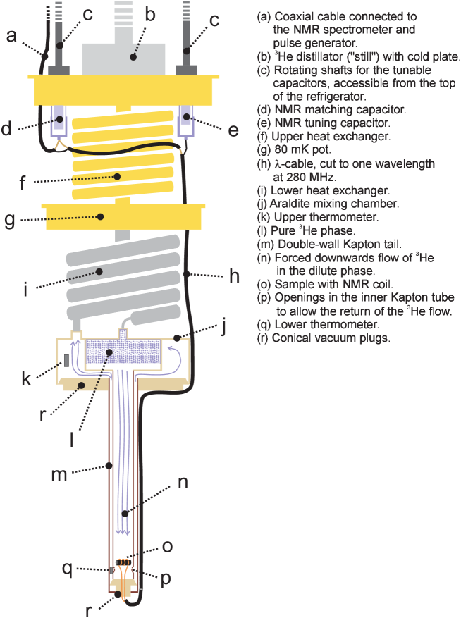
Fig. 2.1 : Scheme of the low-$T$ part of the dilution refrigerator with NMR circuitry. For clarity we omit the vacuum can and the radiation shields anchored at the still and at the 80 mK pot. Only the narrow tail of the refrigerator is inserted in the bore of a 9 T superconducting magnet (not shown).

Our system is based on a Leiden Cryogenics MNK126-400ROF dilution refrigerator, fitted with a plastic mixing chamber that allows the sample to be thermalized directly by the ³He flow, specially designed for our purposes in collaboration with G. Frossati. A scheme of the low-temperature part of the refrigerator is shown in Fig. 2.1, together with the NMR circuitry (see §2.2.2). The mixing chamber consists of two concentric tubes, obtained by rolling a Kapton foil coated with Stycast 1266 epoxy. The tops of each tube are glued into concentric Araldite pots: the inner pot receives the downwards flow of condensed ³He and, a few millimeters below the inlet, the phase separation between pure ³He phase and dilute ³He/⁴He phase takes place. The circulation of ³He is then forced downwards along the inner Kapton tube, which has openings on the bottom side to allow the return of the ³He stream through the thin space in between the tubes. Both the bottom of the Kapton tail and the outer pot are closed by conical Araldite plugs smeared with Apiezon N grease. The Kapton tail is about 35 cm long and is surrounded by two silver-coated brass radiation shields, one anchored at the 80 mK pot, the other at the still. The whole low-$T$ part of the refrigerator is closed by a vacuum can, which has itself a thin brass tail to surround the Kapton part of the mixing chamber, and is inserted into the bore of an Oxford Instruments 9 Tesla NbTi superconducting magnet. In this way, only Kapton and brass cylinders (plus the lowest Araldite plug) are placed in the high-field region, whereas all other high-conductivity metal parts (heat exchangers, 80 mK pot, ³He distillator, etc.) are outside the magnet bore and subject only to a small stray field. This design was intended to minimize eddy currents heating while moving the refrigerator through the pick-up coil of the SQUID magnetometer (§2.4), while thermalizing the sample directly by the contact with the ³He flow. As it turned out, the excellent thermalization obtained is this way is also essential for the success of the NMR experiments described in chapter IV, whose significance depends crucially on the efficient cooling of the nuclear spins (§4.4).

The temperature inside the mixing chamber is monitored by measuring with a Picowatt AVS-47 bridge the resistance of two Speer carbon thermometers, one in the outer top Araldite pot, the other at the bottom of the Kapton tail, just beside the sample. We have verified that the temperature is very uniform along the whole chamber (except in the presence of sudden heat pulses): even at the lowest $T$, the mismatch between the measured values is typically $\lesssim 0.5$ mK. A Leiden Cryogenics Triple Current Source is used to apply heating currents to a manganin wire, anti-inductively wound around a copper joint just above the ³He inlet in the mixing chamber. In this way we can heat the incoming ³He stream and uniformly increase the mixing chamber temperature.

For the ³He circulation we employ an oil-free pumping system, consisting of a Roots booster pump (Edwards EH500) with a pumping speed of 500 m³/h, backed by two 10 m³/h dry scroll pumps (Edwards XDS10). The main pumping line is a $\varnothing$ 100 mm solid tube, fixed at one side with a flexible rubber joint that allows for an inclination of a few degrees, and connected to the head of the fridge by a “T” piece with two extra rubber bellows, to reduce the vibrations transmitted by the pumping system. In this configuration, the system reaches a base temperature that can be as low as 9 mK; with the extra wiring for NMR experiments, the base temperature is $\sim 12$ mK, and the practical operating temperature while applying $rf$-pulses is 15 - 20 mK (see §2.2.3). The typical ³He circulation rate at the base temperature is $\dot{n}\sim 350$ $\mu$mol/s, and the cooling power at 100 mK is $\dot{Q}\sim 150$ $\mu$W. When the Kapton tail is replaced by a flat plug, $\dot{Q}$ can be increased up to 700 $\mu$W @ 100 mK and $\dot{n}\sim 1200$ $\mu$mol/s by applying extra heat to the still; with the tail in place it’s more difficult to increase the circulation rate, and $\dot{Q}$ @ 100 mK hardly exceeds 250 $\mu$W.

2.2 Nuclear Magnetic Resonance

The NMR technique is applied since more than 50 years [22] to widely different research fields; in this thesis, we are interested in the use of nuclear spins as local probes for magnetic fluctuations in solid-state systems, but also in the dynamics of the nuclei themselves, which appears to play an essential role in the quantum behavior of single-molecule magnets.

2.2.1 Basics of pulse NMR

The Hamiltonian of a nuclear spin $\vec{I}$ placed in a magnetic field $\vec{B}_{z}$ applied along a certain axis $\vec{z}$ is:

$$\mathcal{H}=\hbar\gamma\vec{I}\cdot\vec{B}_{z},$$ (2.1)

where $\gamma$ is the gyromagnetic ratio, such that $\mu=\hbar\gamma I$ is the magnetic moment of the nucleus. The eigenstates $|m\rangle$ are the $2I+1$ projections of the spin along $\vec{z}$, having energies $E_{m}$, $m=-I\ldots I$, separated from each other by the Zeeman splitting $E_{m+1}-E_{m}=\hbar\gamma B_{z}$, which corresponds to the Larmor frequencies $\omega=\gamma B_{z}$ for the classical precession. Transitions between adjacent Zeeman levels can be produced by introducing a time-dependent field $\vec{B}_{rf}(t)$, provided that the matrix elements $\langle m|B_{rf}|m+1\rangle\neq 0$, i.e. $\vec{B}_{rf}$ is not parallel to $\vec{z}$. Considering for simplicity a spin $I=1/2$ and taking $\vec{B}_{rf}(t)=B_{rf}\vec{x}\cos(\omega_{N}t)$, the expectation value of the $z$ component of the magnetic moment will oscillate in time at a frequency $\omega_{\mathrm{Rabi}}=\gamma B_{rf}$ (Rabi oscillations):

$$\langle\mu_{z}(t)\rangle=\langle\mu_{z}(0)\rangle\cos(\omega_{\mathrm{Rabi}}t).$$ (2.2)

In a classical picture, this means that, if $\vec{\mu}(0)=\hbar\gamma I\vec{z}$, after a time $t_{\pi/2}=\pi/(2\gamma B_{rf})$ the magnetic moment has been turned 90^∘ away from the $\vec{z}$ axis and lies in the $xy$ plane. For this reason, the application of such an alternating field of frequency $\omega_{N}$ for a time $t_{\pi/2}$ is called “$\pi/2$-pulse”. The rotation angle can in fact take any value, by choosing the appropriate duration and strength of $B_{rf}$. After a $\pi/2$-pulse the state of the system is $|\psi\rangle=1/\sqrt{2}(|+1/2\rangle+|-1/2\rangle)$, and the time evolution caused by the Hamiltonian (2.1) is equivalent to the classical Larmor precession of the magnetic moment within the $xy$ plane, which produces a rotating magnetic field that can be detected via the electromotive force induced in a pick-up coil with axis $\parallel\vec{x}$. In practice the same coil is used to produce $B_{rf}$ and to detect the Larmor precession.

Since we always work with macroscopic ensembles of spins, it is convenient to describe the system in terms of its density matrix $\rho$. If the state of each spin in the system is described as $|\psi\rangle=\sum_{m}a_{m}|m\rangle$, then the matrix elements $\rho_{m,m^{\prime}}$ are the average over the sample of $a_{m}a_{m^{\prime}}^{*}$. The diagonal elements of $\rho$ represent the populations of the levels, and the non-diagonal elements account for the correlation between different spins. Under thermal equilibrium at a temperature $T$, the non-diagonal terms of $\rho$ are zero, and the diagonal terms obey:

$$\frac{\rho_{m,m}}{\rho_{m+1,m+1}}=\exp\left(-\frac{\hbar\gamma B_{z}}{k_{B}T}\right),$$ (2.3)

which corresponds to a longitudinal ($\parallel B_{z}$) nuclear magnetization, $M_{z}(T)$, according to the Curie law:

$$M_{z}(T)=N\hbar^{2}\gamma^{2}\frac{I(I+1)B_{z}}{3k_{B}T},$$ (2.4)

where $N$ is the number of spins per unit volume.

By means of rf-pulses as described above, it is possible to perturb the system and change its density matrix. For instance, the effect of a $\pi$-pulse on an ensemble of spins $1/2$ in thermal equilibrium is to invert the diagonal elements of $\rho$, i.e. the nuclear magnetization. After the inversion, the thermal equilibrium can be reestablished in the presence of perturbations that induce transitions between the Zeeman levels, and of a reservoir that can absorb the heat released by the nuclear spins. The time constant for the recovery of the equilibrium values of the diagonal elements of $\rho$ is $T_{1}$, the nuclear spin-lattice relaxation time.

Far from equilibrium, it is possible to define a nuclear spin temperature $T_{\mathrm{nucl}}$ different from the lattice $T$, provided that the ratio of the populations formally obeys a relation like (2.3) with $T_{\mathrm{nucl}}$ replacing $T$, and that $\rho_{m,m^{\prime}}=0$ for $m\neq m^{\prime}$. For example, a $\pi$-pulse on a spin 1/2 produces a negative spin temperature. $T_{1}$ can be then interpreted as timescale for the reequilibration of the spin- and lattice temperatures.

After a $\pi/2$ pulse, the diagonal elements of $\rho$ are identical and nonzero non-diagonal elements appear. This means that the spins are coherently precessing, the correlation between the single Larmor precessions decaying with a time constant $T_{2}\leq T_{1}$, which is also the decay time for the non-diagonal elements of $\rho$.

In a real experiment, the signal produced by the Larmor precession after a $\pi/2$-pulse, called “free induction decay”, actually decays on a time $T_{2}^{*}\leq T_{2}$ because of static field inhomogeneity, i.e. the fact that spins in different spatial positions may have different $B_{z}$, thus different $\omega_{N}$. This static dephasing can be recovered by means of spin echo. By applying a $\pi$-pulse at a time $\tau>T_{2}^{*}$ after the $\pi/2$-pulse, each spin is rotated 180^∘ about the axis of the coil. In this way, the spins that are precessing “too slow” find themselves ahead of the fast ones. At time $2\tau$ all spins are again precessing in phase (Fig. 2.2), giving rise to an echo of coherent precession whose amplitude depends on the effective correlation $\propto\exp(-2\tau/T_{2})$ at that instant. We can therefore measure $T_{2}$ by applying a $\pi/2-\pi$ pulse sequence with increasing values of $\tau$, and observing the $\tau-$dependence of the echo amplitude.

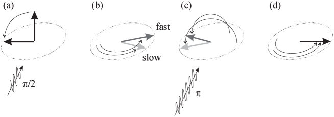
Fig. 2.2 : Sketch of the spin-echo sequence: (a) $\pi/2$-pulse; (b) Larmor precession and dephasing of the slow (light gray) and fast (dark gray) spins; (c) $\pi$-pulse; (d) refocusing of the precessions and formation of the echo.

As regards $T_{1}$, we remark that the coil is sensitive only to the projection of the Larmor precession along its axis, i.e. $\perp\vec{z}$. The effect of a $\pi/2$-pulse, or of an echo sequence, is indeed to project the $z$-component of the nuclear magnetization into the $xy$ plane and make it measurable. For instance, an echo sequence after a $\pi$-pulse yields a signal which is proportional to the initial magnetization, but with opposite phase as compared to the signal without $\pi$-pulse. By introducing a waiting time $\tau$ between the $\pi$-pulse and the echo sequence, one can access the time evolution of the $z$-component of the magnetization, i.e. the recovery of the equilibrium state and thereby the time constant $T_{1}$. A sketch of the pulse sequences used to measure $T_{1}$ and $T_{2}$ is shown in Fig. 2.3.

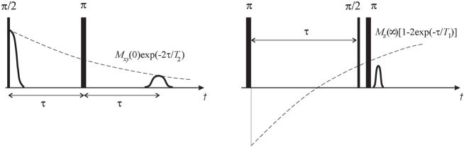
Fig. 2.3 : Left: $T_{2}$ measurement by echo decay. Right: $T_{1}$ measurement by inversion recovery.

2.2.2 Instruments and circuitry

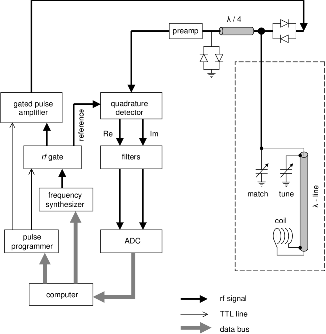
Fig. 2.4 : Scheme of the NMR setup. The parts enclosed in the dashed box are inserted in the dilution refrigerator.

Fig. 2.5 : Time evolution of the mixing chamber temperature while applying 12 $\mu$s - 24 $\mu$s spin-echo pulse sequences. (a) Response of the thermometer at the bottom of the Kapton tail, next to the sample, after two spin-echo sequences at 10 min intervals. (b) Like (a), after 20 sequences at 1 min intervals. (c) Thermometer at the top of the mixing chamber, close to the ³He outlet, after a single spin-echo sequence.

A scheme of the NMR setup used for the present work is shown in Fig. 2.4. The non-commercial electronic devices have been developed by R. Hulstman, and a computer running a Pascal management program written by J. Witteveen [23] controls the generation of the NMR pulses and the detection of the signal. The pulse sequences are obtained by programming a home-made device, which opens the gate of the pulse amplifier (Kalmus 166UP) at the specified times: one typically waits $5$ $\mu$s before the full power of the amplifier (typ. $\sim 100$ W) is available, and closes the gate as soon as the power is no longer necessary, to avoid leakage currents to the NMR coil. The rf-signal to be amplified is generated by the frequency synthesizer (Farnell SSG1000), but is first handled by a rf-gate, driven by the pulse programmer. The purpose of the rf-gate is to produce pulses of the desired length and phase. For instance, to measure a spin echo we first produce a $\pi/2-\pi$ sequence with all the pulses in phase with the reference signal, and record the result; then we repeat the sequence but now with a $180^{\circ}$ phase shift on the $\pi/2$-pulse, and we subtract the measured signal from the previous one. In this way, the “true” NMR signal from the second sequence, which has opposite sign with respect to the first because of the phase shift in the $\pi/2$-pulse, is actually added to the first one, whereas we cancel out the offset of the spectrometer and the ringing (i.e. the fictitious signal that appears because of the electrical resonance of the circuit) produced by the $\pi/2$-pulse [24]. The amplified pulses are then fed to the resonant circuit.

The circuitry we used includes two tunable cylindrical teflon capacitors, mounted at the still of the dilution refrigerator (see Fig. 2.1) and driven by rotatable shafts. The capacitor in parallel to the rf-line is used to match the impedance of the circuit to $50$ $\Omega$, whereas the one in series to the NMR coil tunes the frequency of the resonator. The peculiarity of our circuit is that, because of the distance ($\sim 50$ cm) separating the capacitors from the NMR coil in the mixing chamber, we had to introduce a $\lambda$-cable between coil and tuning capacitor. At the frequency where the cable is precisely one wavelength, the circuit is indeed identical to the standard concentrated circuit. Away from the $\lambda$-frequency, the cable adds extra inductance or capacitance. More importantly, since the $\lambda$-cable is a low-conductivity thin brass coax for low-$T$ applications, the quality factor of the resonator (which includes the cable!) is drastically reduced. Although this affects the sensitivity of the circuit, it also broadens the accessible frequency range without need to retune the capacitors. We found that, cutting the cable for one wavelength at $\sim 280$ MHz, the circuit is usable between (at least) 220 and 320 MHz. Once the desired frequency range is chosen and the $\lambda$-cable is cut accordingly, the NMR coil must be constructed by first mounting it just near the tuning capacitor, i.e. making a “standard” concentrated circuit. If this circuit resonates in the same range as the $\lambda$-frequency, the coil can be safely moved into the mixing chamber.

The NMR signal induced in the coil is first passed though a low-noise DOTY preamplifier placed at the top of the cryostat, then detected by a phase-sensitive quadrature detector, and finally stored in the memory buffer of a flash A/D converter. The results of the positive and negative pulse sequences are subtracted and dumped in the measurement data file. The diodes in parallel to the preamplifier and the $\lambda/4$-cable, together with the diodes in series to the power line, are used to separate the small NMR signal from the high-power pulses. For the pulse amplifier, the diodes in series are a short circuit, whereas the $\lambda/4$-cable is an open circuit since it is short-circuited at the opposite end by the diodes in parallel. In this way all the power goes in the resonator and does not damage the preamplifier. Conversely, the series diodes are an open circuit for the very small signal picked up by the NMR coil, which is therefore entirely conveyed towards the preamplifier.

2.2.3 Heating effects

Applying NMR pulses of typically 100 W for several microseconds to a copper coil at $T\simeq 15$ mK is potentially very harmful for the thermal stability of the sample and of the ³He/⁴He mixture in which it is immersed. As discussed in §2.1, our setup is specially designed to circumvent this problem. In Fig. 2.5 we show three examples of the magnitude of the heating effects that arise when applying spin-echo NMR pulse sequences consisting of a 12 $\mu$s $\pi/2$-pulse followed by a 24 $\mu$s $\pi$-pulse after 45 $\mu$s. Panels (a) and (b) show the temperatures as measured by the thermometer placed at the bottom of the Kapton tail, just next to the NMR coil and the sample, whereas the temperature in panel (c) is taken at the top of the mixing chamber in the outer part of the wide Araldite pot, i.e. 35 cm past the sample in the ³He path. In both cases, a very sharp peak in $T$ is visible at the instant when the pulses are applied, which is simply due to the direct (and instantaneous) heating of the thermometers by the electromagnetic field produced by the coil, thus it does not reflect a “real” increase in the temperature of the ³He bath. The situation is particularly clear in panel (c), where the radiative heating spike is quickly recovered, and only after a few minutes the wave of warmer ³He atoms comes along. By comparing (a) and (b) with (c), it is also clear that the height of the radiative spike is lower in the upper thermometer, which is indeed farther away from the coil. Panel (a) demonstrates that, with an interval of 10 minutes between the sequences, the temperature of the sample can be kept very stable at $\simeq 15$ mK. Even with just 1 minute waiting time (b), the increase of the baseline of the ³He bath temperature does not exceed 5 mK!

2.3 ac - susceptometer

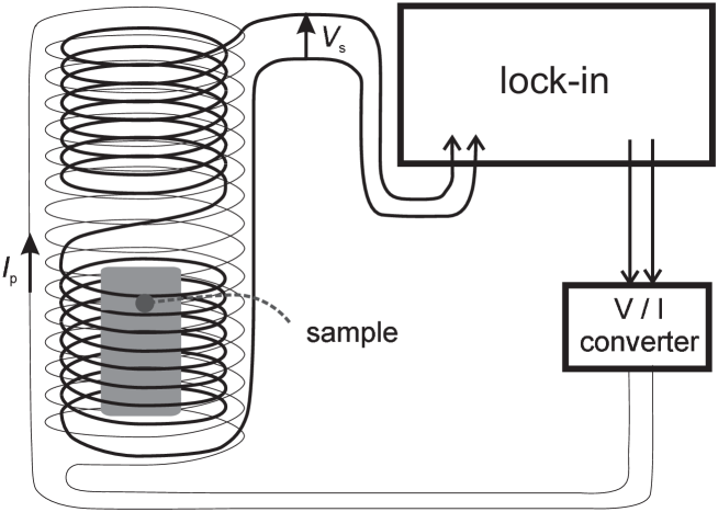
Fig. 2.6 : Schematic drawing of the ac-susceptometer.

For the frequency-dependent ac-susceptibility measurements reported in chapter V we used a simple and compact home-made susceptometer based on the mutual inductance principle. A sketch of the instrument is shown in Fig. 2.6. A primary coil, consisting of $250$ turns of $\varnothing$ $100$ $\mu$m NbTi superconducting wire is wound on top of two secondary coils, each consisting of 600 turns of $\varnothing$ $40$ $\mu$m copper wire, and connected in series with opposite polarity. When an alternating current $I_{p}(t)=I_{p}\cos(\omega t)$ is passed through the primary coil, it induces a voltage $V_{s}=V_{1}-V_{2}$ in the secondary, where $V_{1}$ and $V_{2}$ are the voltages at each section of the secondary coil, and the minus sign is due to the opposite winding directions:

$$V_{s}=\omega I_{p}(\mathcal{M}_{1}-\mathcal{M}_{2})\cos(\omega t+\pi/2).$$ (2.5)

The above relation holds if there is no current flowing in the secondary coils, e.g. when they are connected to an ideal voltmeter. The mutual inductances are given by $\mathcal{M}_{i}=(1+\chi_{i})f$, where ($i=1,2$) and$f=f(N_{p},N_{s},A_{p},A_{s},\ldots)$ is a factor that depends on the geometry, the area and the number of turns of the primary and secondary coils, and $\chi_{i}$ is the magnetic susceptibility of the material filling each secondary coil. By leaving coil 2 empty ($\chi_{2}=0$) and filling coil 1 with the sample to be investigated, we obtain:

$$V_{s}=\omega I_{p}\cos(\omega t+\pi/2)\chi.$$ (2.6)

The susceptibility of the sample is therefore easily measured by connecting the secondary coil to a lock-in amplifier (Stanford SR830); the phase-sensitive detection allows to discern both the real and the imaginary part of the complex susceptibility $\chi=\chi^{\prime}+i\chi"$.

To apply the primary current $I_{p}$ we either introduced a 500 k$\Omega$ resistor in series to the 5 V excitation circuit of the lock-in, or we used a home-built V/I converter that allows to have more current at low frequencies, since the induced voltage is $\propto\omega$. Using the V/I converter we may easily measure down to frequencies $\sim 1$ Hz, whereas above $\sim 1$ kHz it is advisable to simply use the 500 k$\Omega$ series resistor, which eliminates the slight phase rotations that the V/I converter starts to introduce at high frequencies. With a typical value of $I_{p}\sim 50$ $\mu$A, the alternating field produced at the sample is $\mu_{0}H_{p}\sim 1$ $\mu$T.

The susceptometer is small enough to fit vertically in the tail of the dilution refrigerator, or even horizontally in the outer part of the upper Araldite pot (cf. Fig. 2.1), for measurements without static external field.

2.4 SQUID magnetometer

The SQUID magnetometer described in this section is designed to allow high-sensitivity measurements on powder samples down to $T\sim 10$ mK. For example, metallic nanoclusters show spectacular quantum-size effects in their thermodynamic properties [25] at very low temperatures, but their magnetic susceptibility is very small in this regime. Furthermore, most of those materials are highly air-sensitive, thus it is very convenient to introduce and keep the sample in a sealed glass tube, which is also ideal to perform preliminary measurements at $T>1.5$ K in commercial SQUID magnetometers. One of the requirements for the design discussed here is indeed the compatibility with the sealed sample holders used in other experiments, without any need to further manipulate the sample. The really challenging part of the design consists in moving the sample through the pick-up coils while it is at $T\sim 10$ mK inside the mixing chamber of the dilution refrigerator. For samples with such extremely small magnetic signals such a measure is needed because the two components of the pick-up coil will never perfectly compensate one another, leaving an empty-coil signal that could wash out the signal of the sample to be measured. As we shall discuss below, this has required a system that moves the whole dilution refrigerator insert.

2.4.1 Working principle

A SQUID (Superconduting QUantum Interference Device) is basically an ultra-sensitive flux-to-voltage converter, that exploits the peculiar quantum properties of closed superconduting circuits. To understand its working principle, we recall that the superconducting state can be described as the condensation of paired electrons (Cooper pairs) into an ordered phase characterized by a complex order parameter:

$$\psi=|\psi(\vec{r})|e^{i\varphi(\vec{r})},$$ (2.7)

where $|\psi(\vec{r})|^{2}$ is the density of Cooper pairs and $\varphi(\vec{r})=\vec{p}\cdot\vec{r}/\hbar$ is the phase. In the presence of a magnetic field $\vec{B}=\vec{\nabla}\times\vec{\mathcal{A}}$, the generalized momentum is expressed as $\vec{p}=2m\vec{v}-2e\vec{\mathcal{A}}$, since the Cooper pairs have mass $2m$ and charge $2e$ ($e=-1.6\times 10^{-19}$ C).

The current density $\vec{j}$ can be obtained by introducing (2.7) in the standard quantum mechanical expression:

$$\vec{j}=-i\hbar\frac{e}{m}\left(\psi^{*}\vec{\nabla}\psi-\psi\vec{\nabla}\psi^{*}\right)-\frac{4e^{2}}{m}\psi^{*}\psi\vec{\mathcal{A}},$$ (2.8)

$$\vec{j}=\left(\frac{2e\hbar}{m}\vec{\nabla}\varphi-\frac{4e^{2}}{m}\vec{\mathcal{A}}\right)|\psi|^{2}.$$ (2.9)

The current in a superconductor can flow only within a surface layer of thickness comparable to the London penetration depth, since inside the bulk $\vec{j}=0$. By considering a superconducting ring, the integral $\oint\vec{j}\cdot\mathrm{d}\vec{l}$ along a closed path deep inside the bulk is thus obviously zero, i.e.:

$$\oint\left(\frac{2e\hbar}{m}\vec{\nabla}\varphi-\frac{4e^{2}}{m}\vec{\mathcal{A}}\right)\cdot\mathrm{d}\vec{l}=0;$$ (2.10)

recalling the Stokes theorem, $\oint\vec{\mathcal{A}}\cdot\mathrm{d}\vec{l}=\int\int\vec{\nabla}\times\vec{\mathcal{A}}\cdot\mathrm{d}\vec{S}=\int\int\vec{B}\cdot\mathrm{d}\vec{S}=\Phi$ yields the magnetic flux enclosed by the ring. Furthermore, since the order parameter must be single-valued, the total phase accumulated along a closed path must be an integer multiple of $2\pi$:

$$\oint\vec{\nabla}\varphi\cdot\mathrm{d}\vec{l}=2\pi n.$$ (2.11)

Combining (2.10) and (2.11) yields the quantization of the magnetic flux in a superconducting ring:

$$\Phi=n\frac{h}{2e}=n\Phi_{0},$$ (2.12)

where $\Phi_{0}=h/2e=2.07\times 10^{-15}$ Wb is the flux quantum. This means also that, since the externally applied flux $\Phi_{\mathrm{ext}}$ is a classical variable and can be changed smoothly, the quantization of the flux may require a screening current $I_{s}$ to flow in the ring to fulfill the condition:

$$\Phi=\Phi_{\mathrm{ext}}+LI_{s}=n\Phi_{0},$$ (2.13)

where $L$ is the self-inductance of the ring.

A SQUID is obtained by interrupting a superconducting ring with one (rf-SQUID) or two (dc-SQUID) Josephson junctions, i.e. weak links where the superconductivity is locally suppressed but the Cooper pairs can cross by quantum tunneling. The essential feature added by a weak link is that it is no longer possible to find a closed path through the ring such that $\vec{j}=0$ everywhere, since $\vec{j}\neq 0$ through the weak link (Fig 2.7). This adds an extra contribution $\varphi^{\prime}$ to the phase of the order parameter:

$$\varphi^{\prime}=\frac{m}{e\hbar|\psi|^{2}}\int_{w.l.}\vec{j}\cdot\mathrm{d}\vec{l},$$ (2.14)

where the integral is along the weak link, supposed to be so thin that the magnetic flux in negligible, and $|\psi|^{2}$ in the limit of small currents can be taken equal to the bulk value. The condition of single-valued order parameter becomes:

$$\varphi^{\prime}+\frac{2e}{\hbar}\int\int\vec{B}\cdot\mathrm{d}\vec{S}=\varphi^{\prime}+2\pi\frac{\Phi}{\Phi_{0}}=\varphi^{\prime}+2\pi\frac{\Phi_{\mathrm{ext}}+LI_{s}}{\Phi_{0}}=2\pi n.$$ (2.15)

It follows that the screening current $I_{s}(\Phi)$ must be a periodic function of $\Phi_{\mathrm{ext}}/\Phi_{0}$:

$$I_{s}=I_{c}\sin(2\pi\Phi/\Phi_{0})=I_{c}\sin[2\pi(n-\Phi/\Phi_{0})]=I_{c}\sin\varphi^{\prime},$$ (2.16)

which is the famous Josephson phase-current relation. $I_{c}$ is the Josephson critical current, i.e. the maximum supercurrent that can pass through the link without dissipation.

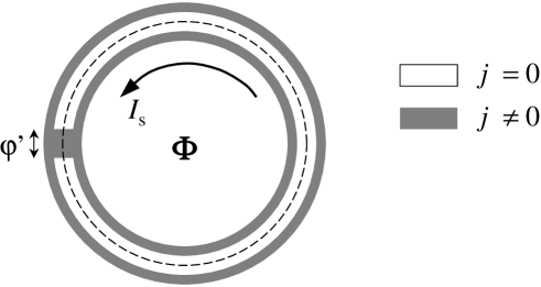
Fig. 2.7 : Sketch of superconducting ring interrupted by a weak link. The dashed line is the integration path.

By applying an external flux which varies linearly in time, a constant voltage $V=-\mathrm{d}\Phi_{\mathrm{ext}}/\mathrm{d}t$ develops across the weak link. Substituting in Eq. (2.16) yields:

$$I_{s}=I_{c}\sin\left(2\pi\frac{Vt+LI_{s}}{\Phi_{0}}\right).$$ (2.17)

This implies that, when a constant voltage is applied to the Josephson junction, an alternating supercurrent circulates in the ring with frequency $\nu=2eV/h$ proportional to the applied voltage. Combining (2.17) and (2.16) we find that a constant voltage produces a linear increase of $\varphi^{\prime}$ with time, i.e. the voltage is proportional to the time derivative of the phase:

$$V=\frac{\hbar}{2e}\frac{\mathrm{d}\varphi}{\mathrm{d}t}.$$ (2.18)

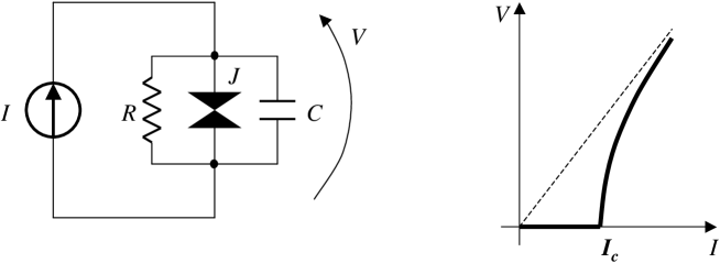
Fig. 2.8 : Model of current-biased Josephson junction (J) with dissipation (R) and capacitance (C), and the relative $V-I$ characteristic.

This relation is useful to obtain the $V-I$ characteristic of a current-biased Josephson junction. When $I>I_{c}$, the current through the weak link causes dissipation, which can be accounted for by a resistance $R$ in parallel to the ideal Josephson junction described by (2.16). Moreover, a realistic junction is formed by two superconducting pads separated by a very thin barrier, so that we have to add a capacitance $C$ to the model. We may then write:

$$I=I_{c}\sin\varphi^{\prime}+\frac{V}{R}+C\frac{\mathrm{d}V}{\mathrm{d}t}=I_{c}\sin\varphi^{\prime}+\frac{\hbar}{2eR}\frac{\mathrm{d}\varphi^{\prime}}{\mathrm{d}t}+\frac{\hbar C}{2e}\frac{\mathrm{d}^{2}\varphi^{\prime}}{\mathrm{d}t^{2}},$$ (2.19)

which leads to a $V/I$ curve of the type shown in Fig. 2.8.

A dc-SQUID, like the one used in our setup, is operated by biasing the junctions $J_{1}$ and $J_{2}$ with a current $I_{\mathrm{bias}}>I_{c}$, such that a voltage develops across them (Fig. 2.9). The essential feature is that the voltage can be modulated by an applied flux, since the critical current $I_{c}$ also depends on $\Phi$. Indeed, after some calculation one finds that the screening current $I_{s}$ is related to the critical current $I_{c}$ of the junctions (assumed to be identical) by:

$$I_{s}=\frac{I_{c}}{2}\left[\sin\varphi_{1}^{\prime}-\sin\left(\varphi_{1}^{\prime}-2\pi\frac{\Phi_{\mathrm{ext}}+LI_{s}}{\Phi_{0}}\right)\right].$$ (2.20)

$I_{c}$ is obtained by maximizing $I_{s}$, yielding the periodic form of $I_{c}(\Phi_{\mathrm{ext}})$ shown in Fig. 2.9. By properly choosing the bias conditions, the dc-SQUID operates therefore as a flux-to-voltage converter, where the external flux can be applied by injecting a current in the input coil. Notice that small a fraction of a flux quantum can produce voltage changes of the order of millivolts! In the practice a dc-SQUID is used in feedback mode by employing a so-called Flux-Lock Loop (FLL), i.e. adding a feedback coil that produces a compensating flux such that $V=const$. This increases the accuracy and the dynamic range of the measurement, and allows to implement noise-reducing detection schemes. For more details on SQUID sensors, see [26, 27].

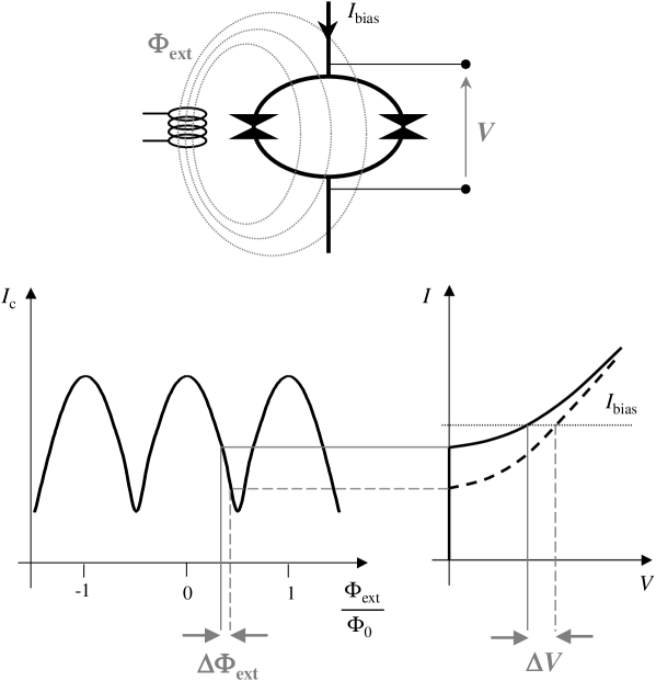
Fig. 2.9 : Working principle of a dc-SQUID as flux-to-voltage converter.

To use a dc-SQUID in an actual magnetometer, it is still necessary to produce a current proportional to the magnetic moment of the sample to be measured. Such a current can be injected in the input coil to produce a flux that is coupled to the SQUID ring by the mutual inductance $\mathcal{M}$. Typically, the input current is obtained by constructing a closed superconducting circuit which includes the SQUID’s input coil on one side, and terminates with a pick-up coil on the other side. Once the circuit has been cooled down below the superconducting critical temperature, the enclosed flux is constant. Any change in the magnetic permeability of the circuit, possibly due to the sample, will result in a screening current that, while keeping the total flux constant, produces the required flux in the input coil. In our case, the change in permeability of the pick-up circuit is obtained by vertically moving the whole dilution refrigerator (§2.4.3), whose tail, that contains the sample, is inserted in the pick-up coil.

Because of the high sensitivity, it is essential to make sure that no sources of flux other than the sample may couple with the SQUID. This can be done by employing a gradiometer, which in its simplest form consists of two coils wound in opposite direction, so that the flux produced by any uniform magnetic field cancels out, and only the gradient of $B$ can be detected (first-order gradiometer). A further improvement is the second-order gradiometer, shown in Fig. 2.10, which is obtained by inserting a coil with $2N$ windings between two coils with N turns each, wound opposite to the central one. This design eliminates also the effects of linear field gradients. Furthermore, according to the reciprocity principle [29], the flux $\Phi$ produced in a coil of arbitrary geometry by a magnetic moment $\mu$ at position $\vec{r}$ is related to the field $\vec{B}(\vec{r})$ produced by the same coil in $\vec{r}$ when carrying a current $I$ such that:

$$\vec{B}\cdot\vec{\mu}=\Phi I.$$ (2.21)

The field produced by a single-loop coil is equivalent to the field of a magnetic dipole, whereas a first-order gradiometer is a magnetic quadrupole, and a second-order is an octupole, so that the fields they produce vary in space like $r^{-3}$, $r^{-4}$ and $r^{-5}$, respectively. From Eq.(2.21) it is clear that a second-order gradiometer is the least sensitive to magnetic fields produced outside of the coil system.

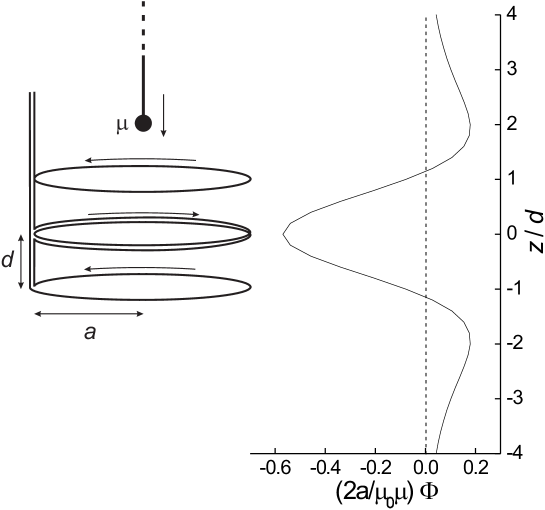
Fig. 2.10 : A second-order gradiometer in Helmoltz geometry ($a=2d$) and the magnetic flux induced by a dipole moving along $z$. Notice that the side peaks in $\Phi(z)$ do not coincide with the positions of the external coils.

The magnetic moment of the sample can be detected by moving it through the pick-up coil. The enclosed flux is easily obtained from the flux induced by a dipole with magnetic moment $\vec{\mu}\parallel\vec{z}$ at a position $z$ along the axis in a loop of radius $a$ placed at $z=z_{0}$:

$$\Phi_{\mathrm{loop}}(z)=\frac{\mu_{0}}{2}f(z-z_{0})\mu,$$ (2.22)

$$f(z-z_{0})=\frac{a^{2}}{[a^{2}+(z-z_{0})^{2}]^{3/2}}=\frac{1}{a}\left[1+\frac{z_{0}^{2}}{a^{2}}\left(\frac{z}{z_{0}}-1\right)^{2}\right]^{-3/2}.$$ (2.23)

If the upper and lower coils of the gradiometer are placed at $z=d$ and $z=-d$, respectively, then the total picked-up flux is:

$$\Phi_{\mathrm{pu}}(z)=N\frac{\mu_{0}}{2}[f(z-d)-2f(z)+f(z+d)]\mu.$$ (2.24)

Typically one adopts the Helmoltz geometry, $a=2d$, resulting in a $\Phi(z)$ as shown in Fig. 2.10.

The picked-up flux is related to the screening current in the circuit, $I_{s}$, by:

$$\Phi_{\mathrm{pu}}=(L_{\mathrm{pu}}+L_{\mathrm{leads}}+L_{\mathrm{in}})I_{s},$$ (2.25)

where $L_{\mathrm{pu}}$, $L_{\mathrm{leads}}$ and $L_{\mathrm{in}}$ are the inductances of the pick-up coil, the leads and the SQUID input coil, respectively. The flux at the SQUID sensor $\Phi_{\mathrm{SQUID}}$ is thus given by:

$$\Phi_{\mathrm{SQUID}}=\mathcal{M}I_{s}=f_{\mathrm{tr}}\Phi_{\mathrm{pu}},$$

$$f_{\mathrm{tr}}=\frac{\mathcal{M}}{L_{\mathrm{pu}}+L_{\mathrm{leads}}+L_{\mathrm{in}}},$$ (2.26)

where $f_{\mathrm{tr}}$ is the flux-transfer ratio [30].

2.4.2 Design and construction of the pick-up circuit

The circuitry for our SQUID magnetometer is, with a few additions, based on the principles discussed above. The niobium dc-SQUID sensor is part of a Conductus LTS iMAG system, which includes a FLL circuitry to be placed just outside the cryostat, and is connected to the SQUID controller by a hybrid optical-electric cable. To couple a magnetic signal to the SQUID we constructed a second-order gradiometer by winding a $\varnothing$ $100$ $\mu$m NbTi wire on a brass coil-holder, to be inserted in the bore of the Oxford Instruments 9 T NbTi superconducting magnet. The gradiometer coils have $\varnothing$ $36$ mm ($a=18$ mm) and $d=9$ mm, due to the $\varnothing$ $34$ mm vacuum can of the refrigerator that contains the sample. The leads of the pick-up circuit, which are tightly twisted and shielded by a Nb capillary, are screwed onto the input pads of the SQUID to obtain a closed superconducting circuit. The input inductance of the SQUID sensor is $L_{\mathrm{in}}=600$ nH; since $L_{\mathrm{leads}}\sim 200$ nH and, given the dimensions, $L_{\mathrm{pu}}\sim L_{\mathrm{in}}+L_{\mathrm{leads}}$ already with $N=1$, it follows from Eq. (2.26) that the most convenient choice of windings for the gradiometer is 1-2-1. The mutual inductance between SQUID ring and input coil is $\mathcal{M}=10$ nH, which means that $f_{\mathrm{tr}}\sim 1/200$.

The FLL included in the Conductus electronics is able to compensate for $500$ $\Phi_{0}$ at the SQUID ring, which means that a maximum flux $\Phi_{\mathrm{pu}}^{\mathrm{(max)}}=500/f_{\mathrm{tr}}\sim 10^{5}$ $\Phi_{0}$ can be picked up by the gradiometer without saturating the system. The maximum magnetic moment $\mu^{\mathrm{(max)}}$ is therefore [cf. Eq. (2.24) and Fig. 2.10]:

$$\mu^{\mathrm{(max)}}\approx\frac{2a}{0.6\mu_{0}}\Phi_{\mathrm{pu}}^{\mathrm{(max)}}\sim 10^{18}\mu_{B}\sim 10^{-2}\mathrm{\ emu}.$$ (2.27)

In order to extend the dynamic range, we have built an extra flux transformer on the pick-up circuit, which allows to introduce a magnetic flux from the outside to compensate for the flux induced by the sample. By using the SQUID as a null-meter, there is the extra advantage that no current circulates in the pick-up circuit, thus the field at the sample is precisely the field produced by the magnet, without the extra field that would be produced by a current in the gradiometer. The flux transformer consists of 16 turns of NbTi wire, wound on top of 1 loop of the pick-up wire and shielded by a closed lead box. In the same box we glued the pick-up leads on a 100 $\Omega$ chip resistor, which is used to locally heat the circuit above the superconducting $T_{c}$ and eliminate the trapped flux. The flux transformer is fed by a Keithley 220 current source, whereas the heater is operated by one of the three current sources in the Leiden Cryogenics Triple Current Source used for the refrigerator; both sources are controlled by a computer program (see §2.4.5)

Despite the efforts to isolate the system from external vibrations, the powerful pumps of the dilution refrigerator still provide a non-negligible mechanical noise. In particular, the Roots pump has a vibration spectrum with a lowest peak at $\sim 25$ Hz. To prevent the possible flux changes induced by such vibrations when coupled to a magnetic field, we added an extra low-pass filter on the pick-up circuit [31] in the form of a 17 mm long $\varnothing$ $0.3$ mm copper wire in parallel with the pick-up leads. At $T=4.2$ K such a wire has a resistance $R\simeq 11$ $\mu\Omega$, which together with the input inductance $L_{\mathrm{in}}=600$ nH of the SQUID yields a cutoff frequency

$$f_{l.p.}=\frac{1}{2\pi}\frac{R}{L_{\mathrm{in}}}\simeq 3\mathrm{\ Hz}.$$ (2.28)

The filter is contained in a separate Pb-shielded box inserted between the flux transformer and the SQUID. The pick-up leads and the copper wire are contacted via Nb pads.

A picture of the SQUID circuitry is shown in Fig. 2.11. The SQUID, the filter and the flux transformer are mounted on a radiation shield of the magnet hanging. The whole system is inserted in a 90 liter helium cryostat. The magnet hanging is stabilized by triangular phosphor-bronze springs (not shown in Fig 2.11) that press against the inner walls of the cryostat.

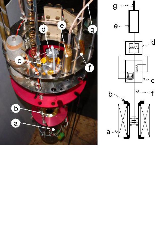
Fig. 2.11 : Picture and scheme of the SQUID circuitry. (a) Superconducting magnet. (b) Coil holder. (c) Flux transformer and heater in lead shield. (d) 3 Hz lead shielded low-pass filter. (e) SQUID sensor. (f) Pick-up leads with Nb capillary shield. (g) SQUID cryocable.

2.4.3 Vertical movement

The movement of the sample through the gradiometer is obtained by lifting the whole dilution refrigerator. For this purpose, the refrigerator is fixed on a movable flange, while the top of the cryostat is closed by a rubber bellow. On the flange we screwed the nuts of three recirculating balls screws (SKF SN3 $20\times 5\mathrm{R}$), which allow a very smooth displacement of the nut by turning the screw. The base of each screw is mounted on ball bearings and is fitted with a gearwheel. The gearwheels are connected by a toothed belt (Brecoflex 16 T5 / 1400) driven by a three-phase AC servomotor (SEW DFY71S B TH 2.5 Nm) that can exert a torque up to 2.5 Nm. In this way, the rotation of the servomotor is converted into the vertical movement of the dilution refrigerator insert. The movement is so smooth that the consequent vibrations are hardly perceptible and do not exceed the vibrations due to the ³He pumping system.

The motor is driven by a servo-regulator (SEW MDS60A0015-503-4-00) that can be controlled by a computer. For safety reasons an electromagnetic brake is fitted, that blocks the motor in case of power failure. In addition, a set of switches is mounted along one of the pillars that support the screws: when the flange reaches the highest or the lowest allowed position, the switches force the motor to brake independently of the software instructions. The maximum allowed vertical displacement is 10 cm.

A picture of the top of the cryostat with the vertical movement elements is shown in Fig. 2.12.

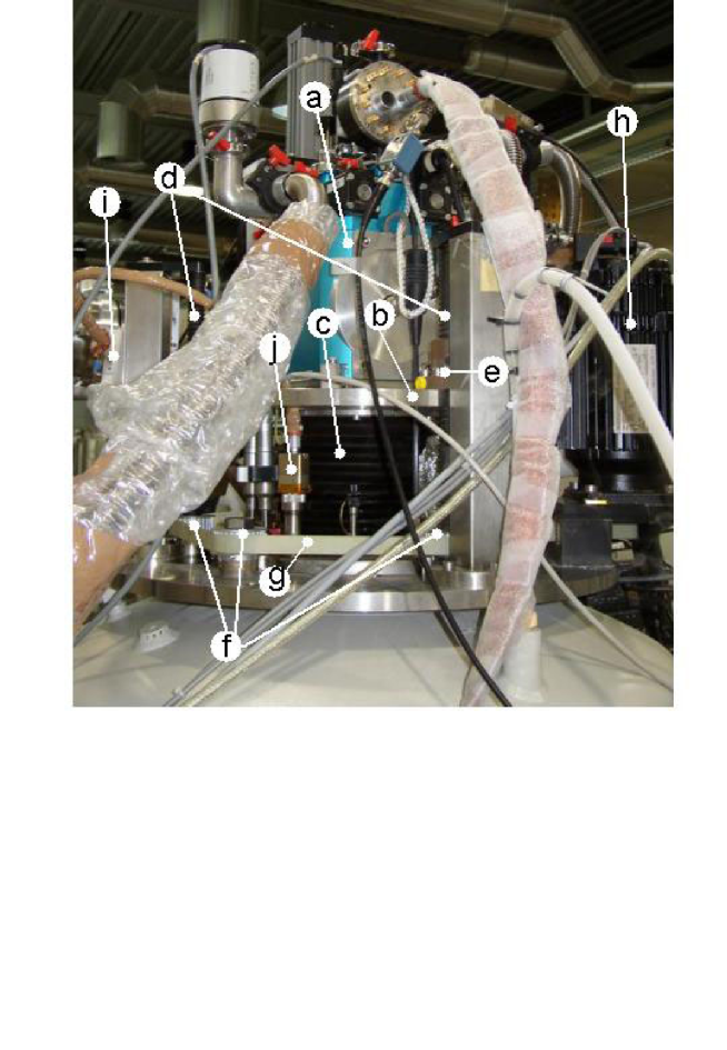
Fig. 2.12 : Picture of the top of the cryostat, with the elements for the vertical movement. (a) Head of the dilution refrigerator. (b) Movable flange. (c) Rubber bellow. (d) Screws. (e) Nut with recirculating balls. (f) Gearwheels. (g) Belt. (h) Servomotor. (i) SQUID FLL electronics. (j) Feedthrough to the SQUID cryocable.

2.4.4 Grounding and shielding

The shielding of the SQUID sensor and electronics is of course a crucial issue for the successful design of a SQUID-based magnetometer. As mentioned in §2.4.2, the low-temperature parts are shielded by superconducting Pb boxes or Nb capillaries. Strange as it may sound, the electronics outside the cryostat posed in fact many more problems. The reason is that the Conductus iMAG system uses beautiful hybrid optical-electric cables for the communication between the SQUID controller and the FLL electronics on top of the cryostat, but in the cable that connects the FLL to the SQUID sensor, the ground is used as return line for the signals! This means that any ground loop involving the SQUID electronics will completely destroy the functionality of the system. Obviously, all the outer metallic parts in the system (e.g. the case of the SQUID sensor, the vacuum feedthrough for the cryocable, etc.) are connected to the same electrical ground, including the GPIB communication terminals.

The best way to avoid ground loops in the SQUID system would be to ground the SQUID sensor and its cable at the cryostat (and take care that it remains a very clean ground), and connect the controller to an isolation transformer [32]. This method is not practicable when communication with the computer via the GPIB bus is needed, and the same computer is connected to another instrument that requires a common ground with the cryostat (this is the case for the Picowatt AVS-47 resistance bridge). The only choice is therefore to ground the controller at its power cord and float the whole SQUID circuitry, all the way to the SQUID sensor inside the cryostat and the shields of the pick-up circuit (which must be connected to the SQUID ground). This is already a rather cumbersome operation, but it’s not yet sufficient. We found out that, in this configuration, the FLL electronics and the room-temperature cables around it are not enough shielded from the electromagnetic interference generated by the motor during the vertical movement of the dilution refrigerator. This sort of interference does not annihilate the functionality of the SQUID like a ground loop would do, nor does it simply induce an increase of the instrumental noise: the effect of bad shielding is that the SQUID system behaves as if it were connected to a non-superconduting, inductive circuit! It obviously took some time before we realized this, since the inductive behavior of the pick-up system is one of the most expectable failures, which can be due to any weakening of the superconductivity in the circuit, for instance because of a bad contact on the SQUID input pads. The full functionality of the magnetometer was reached by enclosing the FLL and the room-temperature SQUID cables into an extra copper shield, grounded at the cryostat but separated from the SQUID ground.

2.4.5 Automation

The operation of the SQUID magnetometer can be programmed in a completely automatic way by a Delphi software developed by W. G. J. Angenent [33], that integrates the SQUID controller, the magnet power supply, the servomotor controller, the thermometers resistance bridge and the current sources for the flux transformer and the pick-up heater.

The software includes a proportional controller that drives the Keithley 220 current source in order to null the SQUID voltage, in case the user chooses the measure in feedback mode rather than just recording the SQUID voltage. Another option is between continuous or step-by-step vertical movement, the latter being more convenient for the feedback measuring mode. Furthermore, the software already contains routines for fitting the SQUID voltage or the feedback current and extract the magnetization. By programming a sequence of, for instance, several measurements at constant temperature and increasing fields, one can obtain a whole magnetization curve without need of any intervention of the user.

A very user-friendly Windows interface is supplied, by which the user can set all the parameters of the measurement, control each single instrument, program measurement sequences and analyze the data. A screenshot of the user interface is shown in Fig. 2.13.

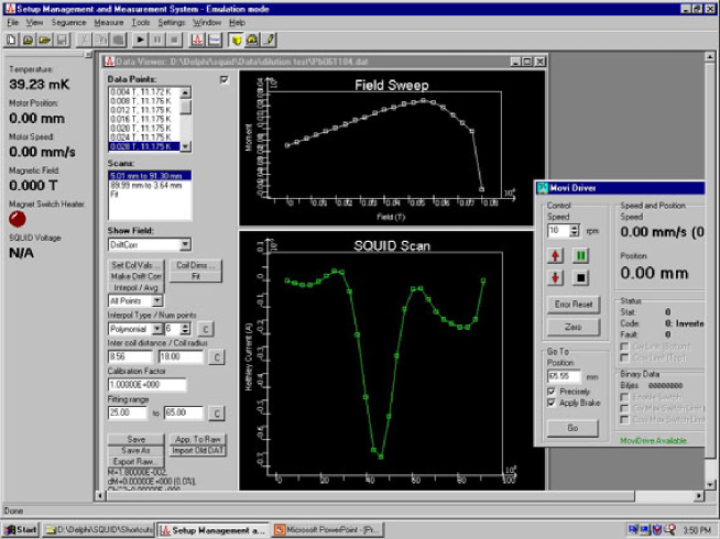
Fig. 2.13 : A screenshot of the user interface of the SQUID magnetometer management program.

2.5 Torque magnetometer

A torque magnetometer (torquemeter, in brief) is the ideal instrument to complement the SQUID on the high-field side, since its sensitivity grows linearly with the field, and it suffers none of the limitations due to the critical field of the superconducting parts of a SQUID magnetometer. We constructed a torquemeter to be installed in a different cryostat, fitted with a 18 T Oxford Instruments Nb₃Sn superconducting magnet and a smaller dilution refrigerator (Oxford Kelvinox 25), which was used previously for specific heat measurements [34]. Again we took care of preserving the compatibility with other setups, namely the calorimeter: the samples used for specific heat experiments can be directly recycled for torque magnetometery.

2.5.1 Principles of cantilever magnetometery

A sample with magnetic moment $\vec{\mu}$ placed in a magnetic field $\vec{B}$ experiences a torque $\vec{\mathcal{T}}$ given by:

$$\vec{\mathcal{T}}=\vec{\mu}\times\vec{B}.$$ (2.29)

The torque is therefore nonzero only if $\vec{\mu}$ is not parallel to $\vec{B}$, which can happen if the sample has an intrinsic magnetic anisotropy and the anisotropy axis is not aligned with the field, or in a single-crystalline isotropic material, provided the crystal itself has a certain shape anisotropy. For a powder isotropic sample, or a non-oriented powder anisotropic sample, $\mathcal{T}=0$. Still, such a sample can experience a force $\vec{F}=\vec{\nabla}(\vec{\mu}\cdot\vec{B})$ if the magnetic field is not uniform. For instance, the magnetic field along the axis ($\vec{z}$) of a magnet has, to a very good approximation, a quadratic dependence on the distance from the field center:

$$B(z)=B_{0}(1-\mathcal{G}z^{2}),$$ (2.30)

where $\mathcal{G}$ is a constant that only depends on the geometry of the magnet coils. The magnetic force on a powder sample is therefore $\vec{F}=(\mathrm{d}B/\mathrm{d}z)\vec{\mu}=-2\mathcal{G}zB_{0}\vec{\mu}$. If the sample is mounted on a torsion cantilever at a distance $r$ from the rotation axis, it exerts a torque:

$$\vec{\mathcal{T}}=-(2\mathcal{G}zB_{0})\vec{r}\times\vec{\mu},$$ (2.31)

which produces a displacement of the extremity of the cantilever $\Delta z=\mathcal{T}/\mathcal{E}$, where $\mathcal{E}$ is an elastic constant. If $\Delta z\ll z$, then $2\mathcal{G}zr/\mathcal{E}=\mathcal{K}$ is just a constant that depends on the cantilever and its position along the magnet. The magnetic moment can therefore be extracted from a measurement of the displacement $\Delta z$:

$$\Delta z=-\mathcal{K}B_{0}\mu.$$ (2.32)

The deflection of the cantilever can be measured in several ways, including piezo-resistive [35] and optical [36] methods, but a simplest effective option is to shape the extremity of the cantilever as a platelet, and measure the changes in the capacitance formed by the platelet facing a suitable counterelectrode [37, 38, 39]. Calling $C_{0}=\epsilon_{0}A/d_{0}$ the capacitance of the system at rest, where $A$ is the area of the platelet and $d_{0}$ the distance at rest from the counterelectrode, the displacement $\Delta z$ produced by the magnetic force translates into a change in the capacitance:

$$\Delta C=C_{0}\left(-\frac{\Delta z}{d_{0}}+\left(\frac{\Delta z}{d_{0}}\right)^{2}+\ldots\right).$$ (2.33)

For a paramagnetic sample and a cantilever placed above the field center, Eq. (2.32) simply implies that the sample is pushed down towards the field maximum, thus if the counterelectrode is below the cantilever, $C$ increases with field. In particular, as long as $\Delta z\ll d_{0}$ so that we can retain only the linear term in (2.33), we may write:

$$\Delta C=\mathcal{K}\frac{C_{0}}{d_{0}}B\mu.$$ (2.34)

The scheme of a typical measurement configuration is shown in Fig. 2.14.

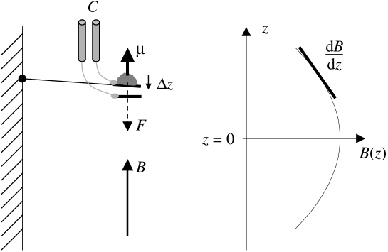
Fig. 2.14 : Scheme of a typical configuration for capacitive detection of the magnetic force on a paramagnetic isotropic sample in a field gradient. The magnitude of the field inhomogeneity is largely exaggerated.

Notice that, at constant $\mu$, the capacitance change (which sets the instrumental sensitivity) grows linearly with field; this is why torque magnetometery is essentially a high-field technique. The magnetic moment is typically obtained by performing field-sweep measurements of the unbalance of a capacitance bridge, then dividing the results by the applied field. Obviously, one should discard the data around zero field, since even the tiniest noise would produce a diverging effect. It is not advisable to perform temperature sweeps at constant field, since the $T$-dependence of $C_{0}$ and $d_{0}$ would affect the results.

2.5.2 Design and construction

From the previous discussion, it is clear that there are several possibilities to increase the sensitivity of a torquemeter: (i) use a soft cantilever (small $\mathcal{E}$); (ii) increase the distance $r$ of the sample from the rotation axis; (iii) build a capacitor with large area and very small distance between the plates; (iv) place the torquemeter far from the field center. The fourth option must be taken with care, and in our case $z$ is determined by the position of the three experimental slots available in the refrigerator [40]: one slot is precisely at the center, the other two are $\sim 25$ mm above and below. The longitudinal inhomogeneity factor [cf. Eq. (2.30)] of the Nb₃Sn magnet used here is $\mathcal{G}\simeq 2.8\cdot 10^{-5}$ T/mm², which means that a torquemeter in the upper slot experiences a field gradient $\mathrm{d}B/\mathrm{d}z\simeq 0.035B_{0}$ T/mm. Contrary to the setup described in §2.1, in this refrigerator the sample is in vacuum, thus it must be thermalized by the cantilever itself.

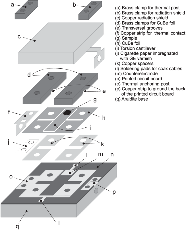
Fig. 2.15 : Drawing of the disassembled torque magnetometer.

The system, shown in Fig. 2.15, lies on an Araldite base, screwed laterally between two wide copper slabs that constitute the cold finger connected to the mixing chamber (not shown). The torquemeter is designed as a symmetric torsion balance, to avoid the possible contribution of the platelet to the magnetic force. The $20\times 4$ mm central strip is held in position by two thin arms, which constitute the elastic twistable element. This cantilever is obtained by spark erosion on a 50 $\mu$m thick copper-beryllium (CuBe) foil, subsequently annealed at 315 ^∘C for two hours in order to eliminate the mechanical stress and obtain a perfectly flat foil. The sample, mixed with Apiezon N grease for thermal contact, is placed at one extremity of the balance, which constitutes the upper plate of the capacitor. The lower plate is obtained from a square copper pad on a printed circuit board. The CuBe foil is held by two brass clamps screwed onto the base, with the interposition of 25 $\mu$m thick copper spacers. The clamps have transversal grooves in correspondence with the torsion arms of the cantilever. To avoid the premature touch of the cantilever on the counterelectrode, we typically put two spacers on top of each other. Pads with the same shape as the spacers are drawn on the printed circuit board; their function is to thermalize the system and to contact electrically the CuBe foil to a coax cable soldered on the board. Since the cantilever constitutes one of the plates of the capacitor and may not be connected to the electrical ground, a L-shaped copper strip is screwed on top of a thermal anchoring post, obtained from teh printed circuit board. A cigarette paper impregnated with GE varnish is inserted between the copper strip and the anchoring post, to provide good thermal contact while maintaining electrical insulation. The copper strip is then screwed laterally between the Araldite base and the cold finger. To shield the sample from thermal radiation and electromagnetic noise we cover the system with a copper box, coated with thin Kapton tape, screwed laterally to the cold finger and therefore also connected to the electrical ground. To complete the shielding, a small copper strip connects the front to the back side of the printed circuit board, which is completely copper-plated.

Two coaxial cables are soldered to copper pads on the printed circuit board, one connected to the counterelectrode, the other to the cantilever. We can therefore measure the capacitance between cantilever and counterelectrode by connecting the coaxials to a General Radio 1615-A capacitance bridge. A Stanford SR830 lock-in amplifier provides the 5 V, $\sim 1$ kHz excitation, and measures the unbalance of the bridge. The measurements are controlled by a LabView program developed by W. G. J. Angenent. Before starting a field-sweep, the temperature is set to the desired value, then the voltage due to the unbalance of the capacitance bridge at zero-field is accurately measured, in order to subtract it from the data afterwards. While sweeping the magnetic field, typically at a rate $\mathrm{d}B/\mathrm{d}t=0.05-0.1$ T/min, the lock-in voltage $V_{L}$ is measured and divided by $B$ after subtraction of the zero-field offset. This yields the sample magnetization $M(B)\propto\mu(B)$, since $V_{L}\propto\Delta C$ [cf. Eq. (2.34)]. The exact conversion factor between the lock-in voltage and the magnetization is very difficult to obtain in a reliable and reproducible way; we shall therefore express $M$ in the “electrical units” $\mu$V/T.

2.5.3 Performance

An example of the performance of our torquemeter is given by the experiment on a $\sim 0.25$ mg Cerium Magnesium Nitrate (CMN) sample, which is an ideal Curie paramagnet down to at least $T\sim 10$ mK.

The measured magnetization, shown in Fig. 2.16(a), exhibits the expected Brillouin behavior up to a certain threshold, where the non-linear terms in (2.33) start to be important. The condition of linear response $\Delta C\propto\Delta z$ is obeyed below a certain maximum displacement, i.e. a horizontal line in the $V_{L}-B$ plane, which translates into a hyperbola in the $M-B$ plane.

By fitting the initial linear part of $M(B)$ at different temperatures, we obtain the static susceptibility $\chi(T)$. As shown in Fig. 2.16(b), the measured susceptibility obeys indeed the Curie law, $\chi\propto 1/T$, and confirms the proper thermalization of the sample.

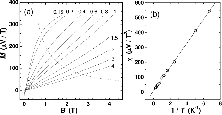
Fig. 2.16 : (a) Magnetization of a 0.25 mg CMN sample, at the indicated temperatures (in Kelvin). Dashed line: (emprical) threshold of the linear response region. (b) Static susceptibility as a function of the inverse temperature, fitted by the Curie law.

Knowing that the magnetization of CMN is $\simeq 3.3$ emu/g at $B=1$ T and $T=1$ K (as deduced from Fig. 14 in [41]), we can estimate that the linear response region is roughly $\mu\cdot B<2\cdot 10^{-3}$ emu$\cdot$T. The instrumental noise, typically $\sim 10$ nV, translates into an equivalent noise of $\sim 10^{-7}$ emu in the magnetic moment at $B=1$ T. By increasing the field to e.g. 10 T, another order of magnitude is gained in the equivalent magnetic noise, but the maximum measurable signal is also 10 times smaller. Therefore, the appropriate amount of sample must be chosen with care, as a function of the range of $B$ and $\mu$ of interest.

Chapter 3 Theoretical aspects of molecular magnetism

This chapter contains a selection of theoretical approaches necessary to understand the physics of molecular magnets and their interaction with the environment. After an introduction to the relevance of this subject for the extrapolation of quantum mechanics to the large scale, we proceed to a “top-down” physical description, starting from the model for a single giant spin in its crystalline environment, then illustrating the effect of a magnetic field and the coupling to nuclear spins and the mutual coupling via dipolar fields. We then discuss the standard theory of the nuclear spin dynamics, mainly to show that such a treatment is no longer adequate in the presence of macroscopic quantum tunneling: the Prokof’ev-Stamp theory is the necessary approach to a unified description of a giant quantum spin coupled to a spin bath. One of the most crucial outcomes of the present work is that even the Prokof’ev-Stamp theory needs an extension in order to account for our experimental results presented in chapter IV. We shall therefore come back to this issue in an extra theoretical section at the end of that chapter.

3.1 Macroscopic quantum phenomena

Besides the perspective of possible applications (magnetic recording media, spin qubits, etc.), single-molecule magnets are very attractive systems to study the observability of quantum phenomena at the macroscopic scale. The motivation behind this interest dates back to the formulation of the Schrödinger cat paradox [4] and the so-called “measurement problem” in quantum mechanics. In fact, the “weak point” of quantum mechanics in its present formulation is the rather artificial distinction between the (microscopic) quantum system and the (macroscopic) measurement apparatus, which is supposed to obey the laws of classical physics, and whose action forces the wave function of the quantum system to be projected (collapse) onto one of its eigenstates. Nothing is specified about where the border between a microscopic (quantum) and a macroscopic (classical) system lies, neither how the collapse of the wave function actually takes place. The proposals to solve these problems range from the most pragmatic idea of decoherence [9], all the way to theories that effectively add extra postulates to the standard quantum mechanics [42, 43]. Before one even attempts to use the experimental observations on SMMs to elucidate the fundamental problems mentioned above, it is essential to quantify the degree of “Schrödinger cattiness” of the quantum states being observed. Here we briefly review the approach of Leggett [44, 10], who usefully introduces two parameters to quantify the macroscopicity of a quantum superposition of states: the “extensive difference” and the “disconnectivity”.

3.1.1 Extensive difference

Let us consider a system in a quantum superposition of states, i.e. whose wave function $|\psi\rangle$ can be expressed as a linear combination of two wave functions:

$$|\psi\rangle=a|\psi_{a}\rangle+b|\psi_{b}\rangle,$$ (3.1)

with the assumption that $|\psi_{a}\rangle$ and $|\psi_{b}\rangle$ represent states of the system which are by some reasonable criterion “classically different”. We may therefore characterize the two branches of the superposition by some extensive quantities $\{i\}$ (e.g. charge, magnetic moment, position of the center of mass, etc.) which should be considerably different in the states $|\psi_{a}\rangle$ and $|\psi_{b}\rangle$. Next, we define $\Lambda_{i}$ as the difference between the values of the extensive quantity $i$ in the two branches of the superposition, divided by a “typical value” of $i$ at the atomic scale (e.g. 1 electron charge, 1 Bohr magneton, 1 Ångstrom, etc.). The “extensive difference” $\Lambda$ of the quantum superposition is then the maximum value assumed among the $\Lambda_{i}$’s.

This sounds at first as a very natural definition of macroscopic distinctness, but in fact it’s easy to find examples where $\Lambda$ is a very large number, although the system is not what one would like to call “macroscopic”. Think of a neutron passing through an interferometer with arms e.g. 10 cm apart: one finds $\Lambda\sim 10^{9}$, although this is clearly not the sort of examples we are looking for as a challenge to the interpretations of quantum mechanics.

3.1.2 Disconnectivity

Leggett introduces therefore another parameter, $\mathcal{D}$, called “disconnectivity”. The precise definition can be found in Ref. [44], but for our purpose it is sufficient to say that $\mathcal{D}$ is the number of particles that have substantially different behavior in the states $|\psi_{a}\rangle$ and $|\psi_{b}\rangle$. More precisely, $\mathcal{D}$ is the number of particle correlations that must be measured in order to distinguish the coherent superposition $|\psi\rangle$ from a statistical mixture of $|\psi_{a}\rangle$ and $|\psi_{b}\rangle$. For instance, a system of $N$ identical particles prepared in a state like

$$|\psi\rangle=a|\psi_{a}\rangle^{N}+b|\psi_{b}\rangle^{N}$$ (3.2)

has $\mathcal{D}=N$, since $N$ particles are simultaneously superimposed, whereas a state

$$|\psi\rangle=(a|\psi_{a}\rangle+b|\psi_{b}\rangle)^{N}$$ (3.3)

has $\mathcal{D}=1$, being just the product of one-particle superpositions. The above-mentioned neutron in a diffractometer has obviously $\mathcal{D}=1$, thereby reestablishing the fact that it does not constitute a “true” macroscopic quantum state. An interesting example is the one of a superconductor: it’s easy to realize that $\mathcal{D}=2$, since the standard BCS wave function is a product of two-particle correlations. The “charge qubit” [45], which is one of the most exciting developments in solid-state quantum devices of the last few years, again has $\mathcal{D}=2$ since it is based on the superposition of a Cooper pair (2 particles) being inside or outside a superconducting island; the fact that the device itself has a size $\sim 1$ $\mu$m does not automatically make it relevant for the problem of quantum mechanics at the large scale!

The observation of high-$\mathcal{D}$ quantum superpositions has been realized only very recently: for instance, by diffraction of C₆₀ molecules [46] a value of $\mathcal{D}=1048$ has been achieved. Even higher values have been reached by the “flux-qubit” [17, 47], which features the superposition of counter-rotating supercurrents in a SQUID loop: in this case all the current-carrying Cooper pairs (i.e. those within the London penetration depth from the surface) are behaving differently in the two branches, yielding $\mathcal{D}>10^{6}$ !

3.1.3 Macroscopicity of a single-molecule magnet

We can now apply the concepts defined above to the case of a SMM. In general, we will be interested in phenomena that arise from the quantum superposition of two different projections of the total spin along the $z$ axis . For example, for Mn₁₂-ac the total spin $S=10$ can give rise to a total magnetic moment of 20 $\mu_{B}$ pointing along $+\vec{z}$ or $-\vec{z}$. A superposition of such two states would be characterized by an extensive difference $\Lambda=40$. As for the disconnectivity, we anticipate (see §3.2.4) that the total spin of the molecule is the result of the ferrimagnetic coupling of 8 Mn³⁺ ions with spin $s=2$, i.e. 4 electron spins per ion, and 4 Mn⁴⁺ ions with $s=3/2$ (3 electrons). In total, the number of electrons having different states when $\vec{S}$ is along $+\vec{z}$ or $-\vec{z}$ is $\mathcal{D}=4\times 8+3\times 4=44$. Although it doesn’t reach the macroscopicity of a fullerene molecule or a SQUID qubit, a SMM is therefore substantially more macroscopic that an atomic-size quantum system.

3.2 Effective Spin Hamiltonian

The magnetic properties of the single-molecule magnets investigated in this thesis are determined in the first place by the net electron spin of each single ion, arising from the partial filling of $3d$ shells. Because of the strong crystal field effects, the electron angular momentum is quenched, so that no orbital contribution needs to be included. Furthermore, the electron spins within a cluster are magnetically coupled by superexchange interactions, typically due to the orbital overlap through oxygen bridges. In this way, one obtains a magnetic ground state which can be characterized by a high value of the total cluster spin $S$, like in the case of Mn₁₂-ac and Mn₆, and is separated from other spin states by an energy determined by the strength of the intracluster superexchange couplings. As long as the temperature is kept much lower than the energy separation between the ground and the first excited total spin state, it is very convenient to adopt the effective spin Hamiltonian description, which means that the cluster is treated as an object characterized by just the number of energy levels compatible with the total spin ground state, i.e. $2S+1$. The resulting energy levels can be further split by the effect of crystal field anisotropy or couplings with magnetic fields. A typical effective spin Hamiltonian to describe the crystal field anisotropy is the following:

$$\mathcal{H}_{\mathrm{CFA}}=-DS_{z}^{2}-BS_{z}^{4}+E(S_{x}^{2}-S_{y}^{2})+C(S_{+}^{4}+S_{-}^{4}).$$ (3.4)

In the next subsections we shall discuss which predictions about the physical behavior of a single-molecule magnet can be made on basis of the above Hamiltonian.

3.2.1 Superparamagnetic blocking

The terms $-DS_{z}^{2}$ and $-BS_{z}^{4}$ (with $|B|\ll|D|$, typically) represent uniaxial anisotropies: if $D>0$, then $z$ is the easy axis of magnetization. In manganese-based clusters the uniaxial anisotropy typically arises from the Jahn-Teller distortion of the coordination octahedra at Mn³⁺ sites; the total cluster anisotropy is then obtained as the vector sum of the single-ion anisotropies [48]. Notice that by considering only these two terms, $\mathcal{H}_{\mathrm{CFA}}$ commutes with the $S_{z}$ operator, thus the eigenstates $|m\rangle$ of $S_{z}$ are also exact eigenstates of $\mathcal{H}_{\mathrm{CFA}}$. The energy levels scheme, as shown in the left panel of Fig. 3.1, can be regarded as a set of doublets of degenerate states, $|+m\rangle$ and $|-m\rangle$, with energies $E_{+m}=E_{-m}$, each state being localized on the left or right side of the anisotropy barrier of height $U$. At temperatures comparable with the barrier height, thermally activated transitions from one side to the other are very fast, and the molecule behaves as a high-spin paramagnet. Since the high spin results from several ions behaving collectively as a single-domain particle, the system is called superparamagnet [49]. The relaxation rate by thermal activation, $\tau^{-1}$, depends on temperature according to the Arrhenius law:

$$\tau^{-1}=\tau_{0}^{-1}\exp(-U/k_{B}T).$$ (3.5)

At sufficiently low temperatures, $\tau^{-1}$ may become exceedingly long and give rise to hysteresis in the magnetization loops [2] and the appearance of a frequency-dependent dissipation peak in the ac-susceptibility [50]. The temperature, $T_{B}$, at which the cluster spin can no longer follow an external driving field is called blocking temperature, and obviously depends on the timescale relevant for the experiment in question.

3.2.2 Spin quantum tunneling

The quantum aspects of SMMs are encountered by considering non-diagonal anisotropy terms like $E(S_{x}^{2}-S_{y}^{2})$, which describes a hard-axis anisotropy caused by a rhombic distortion, and $C(S_{+}^{4}+S_{-}^{4})$ which is the lowest-order non-diagonal term allowed by tetragonal symmetry. These terms do not commute with $S_{z}$, so the eigenstates $|\psi\rangle$ of the complete $\mathcal{H}_{\mathrm{CFA}}$ are no longer a set of doublets of localized states (Fig. 3.1). Expressing $|\psi\rangle$ in the basis of the eigenstates $|m\rangle$ of $S_{z}$:

$$|\psi\rangle=\sum_{m}c_{m}|m\rangle, m=-S\ldots+S,$$ (3.6)

one finds that each doublet now consists of a state $|\psi_{S}\rangle$ with symmetric coefficients, $c_{+m}=c_{-m}$, and an antisymmetric state $|\psi_{A}\rangle$ with $c_{+m}=-c_{-m}$, separated by an energy gap $\Delta=E_{A}-E_{S}$. In particular for the ground doublet, one finds to a very good approximation:

$$|\psi_{S}\rangle = \frac{1}{\sqrt{2}}(|+S\rangle+|-S\rangle)$$

$$|\psi_{A}\rangle = \frac{1}{\sqrt{2}}(|+S\rangle-|-S\rangle).$$ (3.7)

This means that a state localized on one side of the barrier, e.g. $|+S\rangle$, must now be expressed as a superposition of the actual eigenstates:

$$|+S\rangle=\frac{1}{\sqrt{2}}(|\psi_{S}\rangle+|\psi_{A}\rangle).$$ (3.8)

It is clear from basic quantum mechanics [51] that if one would prepare the system at $t=0$ in such a state, $|\psi(t=0)\rangle=|+S\rangle$, the time evolution should obey the Schrödinger equation

$$|\psi(t)\rangle=\frac{1}{\sqrt{2}}e^{-i\frac{E_{S}+E_{A}}{2\hbar}t}(|\psi_{S}\rangle e^{+i\frac{\Delta}{2\hbar}t}+|\psi_{A}\rangle e^{-i\frac{\Delta}{2\hbar}t}).$$ (3.9)

This is equivalent to having coherent oscillations of the cluster spin between the states $|+S\rangle$ and $|-S\rangle$ with frequency $\omega_{T}=\Delta/\hbar$, which implies that the spin is tunneling back and forth through the anisotropy barrier. For this reason the energy gap $\Delta$ is called tunneling splitting.

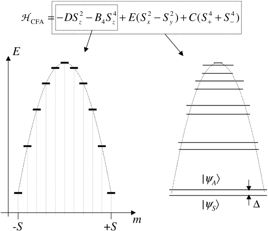
Fig. 3.1 : Sketch of the energy levels scheme for the Hamiltonian (3.4) when considering only the diagonal terms (left) or including the non-diagonal ones (right). The magnitude of the tunneling splittings is largely exaggerated and even not to relative scale.

3.2.3 Coupling with external fields: coherent and incoherent tunneling

It must be stressed that, in real SMMs, the tunneling splitting (particularly the one of the ground doublet) is a very small quantity when produced by non-diagonal anisotropy terms only. As we shall discuss below, the coupling with environmental degrees of freedom is many orders of magnitude larger than $\Delta$, which basically eliminates the possibility to observe coherent tunneling oscillations as described in Eq. (3.9). One of the great advantages of single-molecules magnets as systems to study macroscopic quantum effects, is that the parameters of the spin Hamiltonian, and thereby the whole physical properties, can be easily manipulated by applying an external magnetic field $\vec{B}$. This introduces an extra term in the effective spin Hamiltonian:

$$\mathcal{H}=\mathcal{H}_{CFA}-g\mu_{B}\vec{S}\cdot\vec{B}.$$ (3.10)

By choosing the direction of $\vec{B}$ with respect to the anisotropy axis $\vec{z}$, we have the freedom to either introduce extra non-diagonal terms ($\vec{B}\perp\vec{z}$) that enhance the quantum behavior, or to destroy the symmetry of the energy level scheme ($\vec{B}\parallel\vec{z}$) and thereby reduce the coupling between states on opposite sides of the anisotropy barrier.

Very important for the present discussion is the case where a longitudinal magnetic field $B_{z}(t)$ fluctuates in time and produces a bias, $\xi(t)=2g\mu_{B}B_{z}(t)S$, on the cluster spin doublets. If $\xi(t)$ spans a range much larger than $\Delta$ but crosses several times through the tunneling resonance, one finds that at each crossing there is a nonzero probability for the cluster spin to tunnel through the barrier, but there is no correlation between subsequent tunneling events; therefore this is called “incoherent tunneling”. The probability $P_{\mathrm{LZ}}$ of a single tunneling event upon crossing through the tunneling resonance can be calculated with the Landau-Zener formula [52]:

$$P_{\mathrm{LZ}}=1-\exp\left(\frac{-\pi\Delta^{2}}{2\hbar\mathrm{d}\xi(t)/\mathrm{d}t}\right).$$ (3.11)

A sketch of a Landau-Zener transition is given in Fig. 3.2. This phenomenon has been successfully exploited as a way to extract the tunneling splitting [53, 54] by sweeping an external magnetic field through the tunneling resonance. As will be discussed below, the Landau-Zener formalism can also be used to describe the coupling between a single cluster spin and its environment, since very often the effect of environmental fluctuations can be treated as an effective magnetic field that couples to the cluster spin.

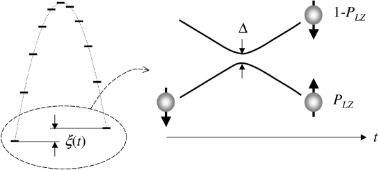
Fig. 3.2 : If the bias $\xi(t)$ crosses the tunneling resonance, the cluster spin may tunnel through the anisotropy barrier with a probability given by Eq. (3.11). The drawing on the right represents the time evolution of a doublet of electron spin levels while crossing the resonance.

In the presence of incoherent tunneling fluctuations, it is essential to distinguish between the average time interval $\tau_{T}$ between subsequent uncorrelated tunneling events, and the so-called tunneling traversal time $\tau_{\mathrm{tr}}$, which is in our case the timescale for the reversal of the cluster spin. A detailed analysis of the tunneling traversal time constitutes a topic on itself [55, 56, 57], but for our purposes it is sufficient to estimate the order of magnitude of $\tau_{\mathrm{tr}}$. In the general framework of the semiclassical instanton technique [6, 58], $\tau_{\mathrm{tr}}$ is related to the inverse of the “bounce frequency” or “attempt frequency” $\Omega_{0}$, i.e. the frequency of the small oscillations at the bottom of each potential well. In SMMs $\hbar\Omega_{0}$ is of the order of the energy separation between the two lowest electron spin doublets, as shown in Fig. 3.3. For instance in Mn₁₂-ac we have $\hbar\Omega_{0}\sim 10$ K, thus $\tau_{\mathrm{tr}}\sim\Omega_{0}^{-1}\sim 10^{-12}$ s. This means that the tunneling events take place in a virtually instantaneous way, as compared to the timescale of all other relevant phenomena.

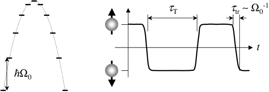
Fig. 3.3 : Illustration of the relationship between tunneling traversal time $\tau_{\mathrm{tr}}$, bounce frequency $\Omega_{0}$ and tunneling interval $\tau_{T}$ for incoherent tunneling of the cluster spin.

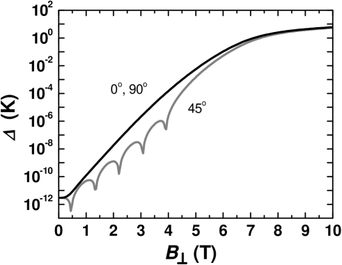
Fig. 3.4 : Perpendicular field dependence of the tunneling splitting of the ground doublet in Mn₁₂-ac, as obtained by numerical diagonalization of the Hamiltonian (3.14). The two lines refer to $\vec{B}_{\perp}$ parallel to the $x$ or $y$ crystallographic axes, or oriented at $45^{\circ}$ between them.

In order to push the system into a regime where coherent tunneling may take place, it is necessary to increase $\Delta$ above the strength of the coupling with environmental degrees of freedom. This can be done by applying a magnetic field $B_{\perp}$ perpendicular to the anisotropy axis. Although sophisticated calculations of $\Delta(B_{\perp})$ have been proposed [59, 60], it is often more practical to obtain $\Delta(B_{\perp})$ directly from the numerical diagonalization of the spin Hamiltonian. An example of the resulting $\Delta(B_{\perp})$ in the case of Mn₁₂-ac is shown in Fig. 3.4. A simplified expression for $\Delta(B_{\perp})$, based on the Hamiltonian $\mathcal{H}=-DS_{z}^{2}-g\mu_{B}\vec{B_{\perp}}\cdot\vec{S}$, has been obtained in the limit $g\mu_{B}B_{\perp}\ll DS$ and $S\gg 1$ by Korenblit and Shender [61]:

$$\Delta(B_{\perp})\approx\frac{4}{\sqrt{\pi}}DS^{3/2}\left(\frac{eg\mu_{B}B_{\perp}}{4DS}\right)^{2S},$$ (3.12)

where $e$ is the base of the natural logarithm. The more general expression for the splitting $\Delta_{m}$ of any doublet of levels $|+m\rangle$, $|-m\rangle$ is [62]:

$$\Delta_{m}(B_{\perp})\approx\frac{2D}{[(2m-1)!]^{2}}\frac{(S+m)!}{(S-m)!}\left(\frac{g\mu_{B}B_{\perp}}{2D}\right)^{2m}.$$ (3.13)

It clearly appears that the simple application of a perpendicular field has an enormous influence on $\Delta$, which allows to study the quantum dynamics of SMMs in different regimes.

From Eq. (3.13) it is also clear that, since $g\mu_{B}B_{\perp}\ll DS$, the tunneling splitting increases drastically (exponentially, in fact) when higher excited doublets (i.e. with lower $|m|$) are considered. Therefore, in the presence of thermal excitations, tunneling can more easily proceed through excited doublets than through the ground state. This remains true in zero external field, although the tunneling splitting is produced by non-diagonal anisotropy terms. The details of the mechanism of thermally-assisted tunneling have generated a vast literature [63, 64, 65, 66, 67], since a large majority of experiments on SMMs have been carried out in the temperature regime $T>1.5$ K, where tunneling through excited states is essential. The transition to pure ground state tunneling happens indeed at temperatures that, at a first sight, appear surprisingly low. The point is that, although the Boltzmann factors for the population of excited doublets are exponentially small, $\Delta_{m}$ grows exponentially upon excitations to higher doublets (3.13), so the competition between the two exponents cannot be treated in a trivial way [68]. Since the present work is focused on the ultra-low temperature regime, the topic of thermally assisted tunneling will be touched upon only marginally.

3.2.4 Parameters for Mn₁₂-ac

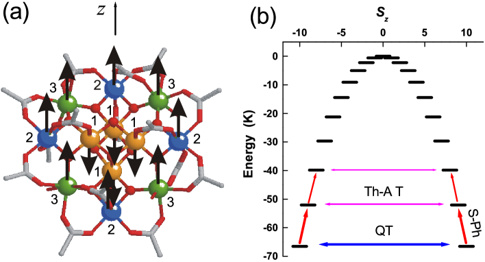
Fig. 3.5 : (a) Structure of the Mn₁₂-ac cluster, with the labelling of the three inequivalent Mn sites as described in the text. (b) Energy level scheme for the electron spin as obtained from the Hamiltonian (3.14), retaining only the terms diagonal is $S_{z}$. The non-diagonal terms allow transitions between states on opposite sides of the anisotropy barrier by means of quantum tunneling (QT). In the presence of intrawell transitions induced by thermal excitation, thermally assisted quantum tunneling (Th-A T) between excited doublets can also take place .

The structure of the [Mn₁₂O₁₂(O₂CMe)₁₆(H₂O)₄] (Mn₁₂-ac) cluster [69] (Fig. 3.5) contains a core of 4 Mn⁴⁺ ions with electron spin $s=3/2$, which we shall denote as Mn⁽¹⁾, and 8 Mn³⁺ ions ($s=2$) on two inequivalent crystallographic sites, Mn⁽²⁾ and Mn⁽³⁾. The electron spins are coupled by mutual superexchange interactions, the strongest being the antiferromagnetic interaction between Mn⁽¹⁾ and Mn⁽²⁾ [70]. The molecules crystallize in a tetragonal structure with lattice parameters $a=b=17.319$ Åand $c=12.388$ Å. Numerical studies have shown the influence of the magnitude and sign of the exchange constants on the precise energy level structure of the cluster [71], and an attempt has been made to verify the assignment of the exchange interactions by a spin-wave analysis of the nuclear spin-lattice relaxation rate in the thermally activated regime [72]. The ground state of the molecule has a total electron spin $S=10$ and is separated from the first excited manifold $S=9$ by $\sim 58$ K, according to neutron scattering experiments [73]. For the temperature range of interest in the present work ($T<2$ K), we may therefore describe the electron spin of the cluster by means of the spin Hamiltonian in the $S=10$ manifold:

$$\mathcal{H}=-DS_{z}^{2}-BS_{z}^{4}+C(S_{+}^{4}+S_{-}^{4})+\mu_{B}\vec{B}\cdot\mathbf{g}\cdot\vec{S}.$$ (3.14)

We adopt the parameter values $D=0.548$ K, $B=1.17\times 10^{-3}$ K and $C=2.2\times 10^{-5}$ K as obtained by neutron scattering data [74], and for the $\mathbf{g}$ tensor the values $g_{\parallel}=1.93$ and $g_{\perp}=1.96$ from high-frequency EPR [75]. The uniaxial anisotropy terms $-DS_{z}^{2}$ and $-BS_{z}^{4}$ can be attributed to the single-ion anisotropy of the Mn³⁺ ions[75], which is due to the crystal field effects resulting in the Jahn-Teller distortions of the coordination octahedra, where the elongation axes are approximately parallel to the $\hat{c}$-axis of the crystal. The energy levels scheme is then a series of doublets of degenerate states which are separated by a barrier with a total height $DS^{2}+BS^{4}\simeq 66.6$ K. The non-diagonal anisotropy term $C(S_{+}^{4}+S_{-}^{4})$ arises from the fourfold $S_{4}$ point symmetry of the molecule, and is the lowest order term that would allow the quantum tunneling of the electron spin between states $S_{z}=\pm m$. An external magnetic field $B_{z}$ parallel to the anisotropy axis would introduce an extra term $g_{\parallel}\mu_{B}B_{z}S_{z}$ in the Hamiltonian, thereby destroying the symmetry of the energy level scheme; at the particular values of field $B_{z}^{mm^{\prime}}=[n/(g_{\parallel}\mu_{B})][D+B(m^{2}+m^{\prime 2})]$, with $n$ an integer $-S\leq n\leq S$, the states $S_{z}=m$ on one side of the barrier come in resonance with the states $S_{z}=m^{\prime}=n-m$ on the opposite side. In the presence of nondiagonal terms in the spin Hamiltonian, one then expects the occurrence of quantum tunneling of the magnetization, as indeed observed in the experiments [8]. The selection rules imposed by the term $C(S_{+}^{4}+S_{-}^{4})$ imply that resonant tunneling should be observed only for $n$ a multiple of 4, in contrast with the observation that steps of comparable height appear in the magnetic hysteresis loops for all values of $n$. There is now solid experimental evidence [77, 78] for the prediction [79] that a disorder in the acetic acid of crystallization is present and gives rise to six different isomers of Mn₁₂ cluster, four of which have symmetry lower than tetragonal and therefore possess non-diagonal anisotropy terms that would allow tunneling transitions for any even value of $n$. Furthermore, to obtain tunneling resonances also at odd values of $n$, it is necessary to introduce in (3.14) the effect of dipolar fields originating from neighboring molecules and the hyperfine couplings with the nuclear spins, as will be described below.

A peculiarity of the Mn₁₂-ac system is the presence in every real sample of fast-relaxing molecules (FRMs) [80], i.e. clusters characterized by a lower anisotropy barrier and a much faster relaxation rate, as observed for instance by ac-susceptibility [81] and magnetization measurements [82]. It has been recognized that such FRMs originate from Jahn-Teller isomerism[83], i.e. the presence in the molecule of one or two Mn³⁺ sites where the elongated Jahn-Teller axis points in a direction roughly perpendicular instead of parallel to the crystalline $\hat{c}$-axis. This results in the reduction of the anisotropy barrier to 35 or 15 K in case of one or two flipped Jahn-Teller axes, respectively[84], and presumably in an increase of the non-diagonal terms in the spin Hamiltonian as well. Furthermore, the anisotropy axis $z$ of the whole molecules no longer coincides with the crystallographic $\hat{c}$-axis, but deviates e.g. by $\sim 10^{\circ}$ in the molecules with 35 K barrier[82]. The Jahn-Teller isomerism is very different from the above-mentioned effect of disorder in solvent molecules, and produces much more important effects. As shall become clear in chapter IV, the presence of the FRMs is essential for the interpretation of our experimental data.

3.2.5 Parameters for Mn₆

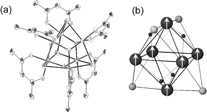
Fig. 3.6 : (a) Crystal structure of Mn₆O₄Br₄(Et₂dbm)₆ [85]. (b) Detail of the symmetric octahedral core, containing six ferromagnetically coupled Mn³⁺ ions, yielding a total spin $S=12$ for this molecular superparamagnetic particle.

The molecular core of Mn₆O₄Br₄(Et₂dbm)₆, hereafter abbreviated as Mn₆ [85], is a highly symmetric octahedron of Mn³⁺ ions (with spin $s=2$) that are ferromagnetically coupled via strong intra-cluster superexchange interactions (Fig. 3.6). Accordingly, the ground state is a $S=12$ multiplet and the energy of the nearest excited state is approximately $150$ K higher. The unit cell is monoclinic, with space group Pc and contains $4$ molecules bound together only by Van der Waals forces. Inter-cluster superexchange is therefore negligible and the only relevant interaction interaction between cluster spins is the dipolar one.

To determine the spin Hamiltonian of the $S=12$ manifold, we notice that the anisotropy of the single Mn³⁺ ions may be very strong due to Jahn-Teller effects. On the other hand, due to the highly symmetric octahedral structure of the cluster, the addition of the single-ion anisotropies may lead to a vanishingly small net cluster anisotropy, no matter how large is the zero-field splitting of the constituting atoms [48]. Indeed, the analysis of magnetization data on basis of the simple Hamiltonian:

$$\mathcal{H}=-DS_{z}^{2}-g\mu_{B}\vec{B}\cdot\vec{S}.$$ (3.15)

indicated an upper limit $|D|\lesssim 0.01K$ for the total cluster anisotropy [85], with $g\simeq 1.94-1.98$. An independent estimate of $D$ was obtained by high-frequency ESR data taken in the range $95-380$ GHz by J. Krzystek (NHMFL Tallahassee, USA) [86]. Owing to the combination of very small $D$ and large $S$, as well as the presence of a signal at $g=2.00$ arising from a minute amount of Mn²⁺ impurity (often seen in ESR of Mn³⁺ compounds), the interpretation of the spectra was not fully conclusive. Nevertheless, signals with a clearly visible structure on the low-field end of the spectra could be obtained. It could be identified as fine structure originating from zero-field splitting (ZFS), since it was independent of field and frequency. Simulations of the spectra performed using Eq. (3.15) agree well with the experiment taking $|D|/k_{B}\sim 0.03$ or $\sim 0.05$ K, depending on the sign of $D$ (which could not be unequivocally determined). Although a smaller rhombic component could be present, the data do not justify a more elaborate fitting.

The Mn₆ cluster constitutes therefore a practical example of how the anisotropy parameters of high-spin molecules can be tuned by simply modifying the crystal structure, while maintaining the same constituents as other clusters having very different properties (cf. Mn₁₂-ac in §3.2.4).

3.3 Hyperfine couplings

The coupling between electron and nuclear spins in a single ion can be generally expressed in the form:

$$\mathcal{H}_{\mathrm{hyp}}=\vec{I}\cdot\mathbf{A}\cdot\vec{s}=-\gamma_{N}\hbar\vec{I}\cdot\vec{B}_{\mathrm{hyp}}$$ (3.16)

where $\vec{I}$ is the nuclear spin, $\vec{s}$ is the electron spin of the single ion, $\mathbf{A}$ is the hyperfine coupling tensor, $\gamma_{N}$ is the nuclear gyromagnetic ratio and $\vec{B}_{\mathrm{hyp}}$ is the total hyperfine field at the nucleus. The hyperfine tensor can contain several contributions depending on the particular nuclear site under consideration. For instance, $\mathbf{A}$ for the ⁵⁵Mn nuclei in a Mn⁴⁺ ion is a diagonal tensor: the only contribution comes from the the isotropic Fermi contact term, arising from the core polarization of inner $s$ electrons caused by 3$d$ electron spins. For the ¹H nuclei, located at the ligands of the molecules, the main contribution is instead arising from the dipolar field produced by the electron spins. The resulting $B_{\mathrm{hyp}}$ is then typically much smaller than for ⁵⁵Mn.

3.3.1 Hyperfine fields on the ⁵⁵Mn nuclei in Mn₁₂-ac

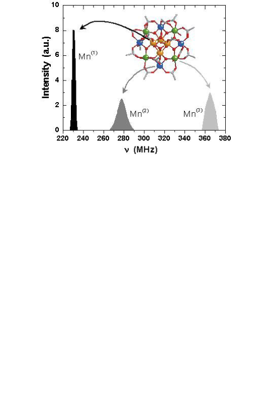
Fig. 3.7 : ⁵⁵Mn NMR spectra in zero field, with assignment of each line to the corresponding site in the molecule (adapted from [87]).

Thanks to the high anisotropy barrier of Mn₁₂-ac, it is possible to detect the Larmor precession of ⁵⁵Mn nuclear spins even in the absence of an external field, by exploiting the local hyperfine field from the electron spins which, below the blocking temperature $T_{\mathrm{B}}\sim 3$ K of the superparamagnetic clusters, is static on the timescale of an NMR experiment. Goto et al.[88] were the first to find that the ⁵⁵Mn NMR spectrum in zero field consists of three quadrupolar-split lines centered around 230, 280 and 365 MHz. The hyperfine fields in each of the three inequivalent Mn sites are directly obtained as $B_{\mathrm{hyp}}=2\pi\nu/\gamma_{N}$, where $\gamma_{N}/2\pi=10.57$ MHz/T is the gyromagnetic ratio of the ⁵⁵Mn nuclei, yielding $B_{\mathrm{hyp}}^{(1)}=21.8$ T, $B_{\mathrm{hyp}}^{(2)}=26.5$ T and $B_{\mathrm{hyp}}^{(3)}=34.5$ T. Subsequently, a detailed analysis of the hyperfine couplings has been reported by Kubo et al.[87], who were able to assign these three NMR lines to specific Mn sites in the molecule. The line centered at $\nu^{(1)}\simeq 230$ MHz corresponds to the nuclei in Mn⁴⁺ ions, and is characterized by a relatively small quadrupolar splitting $\Delta\nu^{(1)}_{Q}\simeq 0.72$ MHz. The direction of $\vec{B}_{\mathrm{hyp}}$ is antiparallel to the Mn⁴⁺ electron spin, thus it coincides with the direction of the total spin $S=10$ of the molecule. In the Mn³⁺ ions, the hyperfine interaction contains also a dipolar term, which makes the coupling tensor anisotropic. Furthermore, $\vec{B}_{\mathrm{hyp}}$ is not exactly antiparallel to the electron spin, but there’s a small canting angle[87]. Accounting for the effects of a dipolar contribution to the hyperfine field in Mn³⁺, it was then possible to assign the line at $\nu^{(2)}\simeq 280$ MHz to the Mn⁽²⁾ site and the line $\nu^{(3)}\simeq 365$ MHz to the Mn⁽³⁾ site[87] (cf. Fig. 3.7). The quadrupolar splittings of these lines are $\Delta\nu^{(2)}_{Q}\simeq 4.3$ MHz and $\Delta\nu^{(3)}_{Q}\simeq 2.9$ MHz

The structure mentioned above is reflected in the effect on the NMR frequencies of an external field $\vec{B}_{z}$ applied along the anisotropy axis. The total field at the nuclear site becomes $\vec{B}_{\mathrm{tot}}=\vec{B}_{\mathrm{hyp}}+\vec{B}_{z}$; in particular for the Mn⁽¹⁾ site (but approximately also for the other sites), since $\vec{B}_{\mathrm{hyp}}$ is parallel to $\vec{B}_{z}$, $\nu(B_{z})=\gamma_{N}(B_{\mathrm{hyp}}+B_{z})=\nu(0)+\gamma_{N}B_{z}$ exhibits a slope[89, 87] which is given by the gyromagnetic ratio of ⁵⁵Mn.

3.3.2 NMR spectra in perpendicular field

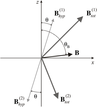
Fig. 3.8 : Sketch of the orientation of hyperfine fields in Mn⁴⁺ ($\vec{B}_{\mathrm{hyp}}^{(1)}$) and Mn³⁺ ($\vec{B}_{\mathrm{hyp}}^{(2)}$) ions, relative to the crystal axes $x$ and $z$ of the molecule, in the presence of an external magnetic field $\vec{B}$ at an angle $\theta_{B}$ from the $z$ axis. The total field at the nuclear site, $B_{\mathrm{tot}}$, which determines the NMR frequency, is obtained as vector sum of $\vec{B}_{\mathrm{hyp}}$ and $\vec{B}$.

If the magnetic field is applied perpendicular to the anisotropy axis, the situation is complicated by the fact that the electron spins, and as a consequence also the hyperfine fields, tend to cant towards the direction of the external field [6]. Recently, Furukawa et al. [90] have analyzed the ⁵⁵Mn NMR spectrum of Mn₁₂-ac in perpendicular fields by assuming that the canting angle $\theta$ between the direction of the electron spins and the $c$-axis of the molecules is given by $\sin\theta=M_{\perp}/M_{s}$, where $M_{s}$ is the saturation magnetization of the $S=10$ ground state, and $M_{\perp}$ is the component of the magnetization along the field direction. At the very low temperatures involved in the present work the contribution of excited electron spin states to the total magnetization is negligible, and the above approach is equivalent to expressing the canting angle as:

$$\sin\theta=\frac{\langle S_{x}\rangle}{10},$$ (3.17)

where $\langle S_{x}\rangle=\langle\psi_{\mathrm{G}}|S_{x}|\psi_{\mathrm{G}}\rangle$ is the expectation value of the $x$-component of the spin in the ground state $|\psi_{\mathrm{G}}\rangle$, to be obtained by numerical diagonalization of the Hamiltonian (3.14). There’s no difficulty in allowing the field $\vec{B}$ to lie at an arbitrary angle $\theta_{B}$ with respect to $\vec{z}$, which helps accounting for the possibility of misalignments between external field an crystal axes. Assuming that the hyperfine field $\vec{B}_{\mathrm{hyp}}$ has always the same strength as deduced from the zero-field spectra and a direction given by the canting angle calculated above, the total field at the nuclear site is obtained as:

$$B_{\mathrm{tot}}=\sqrt{(B_{\mathrm{hyp}}\sin\theta+B\sin\theta_{B})^{2}+(B_{\mathrm{hyp}}\cos\theta+B\cos\theta_{B})^{2}}$$ (3.18)

for Mn⁴⁺ ions and

$$B_{\mathrm{tot}}=\sqrt{(B_{\mathrm{hyp}}\sin\theta-B\sin\theta_{B})^{2}-(B_{\mathrm{hyp}}\cos\theta-B\cos\theta_{B})^{2}}$$ (3.19)

for the Mn³⁺ ions, for which the direction of $\vec{B}_{\mathrm{hyp}}$ is opposite to the total magnetic moment of the cluster (Fig. 3.8). The ⁵⁵Mn Larmor frequency can be directly calculated as:

$$\nu(\vec{B})=\frac{\gamma_{N}}{2\pi}B_{\mathrm{tot}},$$ (3.20)

yielding the field dependence of the Larmor frequencies shown in Fig. 3.9.

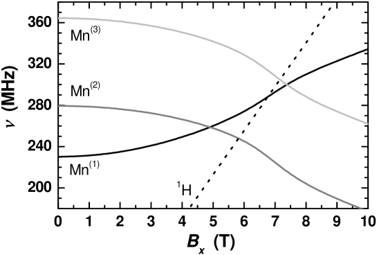
Fig. 3.9 : Perpendicular field dependence of the ⁵⁵Mn resonance frequencies, calculated according to Eqs. (3.18) and (3.19) assuming $\theta_{B}=90^{\circ}$ exactly. For comparison, we also plot the Larmor frequency of ¹H.

The condition $B_{\mathrm{hyp}}(\vec{B})=B_{\mathrm{hyp}}(0)$ for any value of $\vec{B}$, which is contained in Eq. (3.17) and used to derive Eqs. (3.18) and (3.19), is actually equivalent to assuming that the total spin of the molecule $S=\sqrt{\langle S_{x}\rangle^{2}+\langle S_{z}\rangle^{2}}$ remains equal to 10 at all fields. By diagonalizing the Hamiltonian (3.14) one finds that this is the case only if the external field is not exactly perpendicular to $\vec{z}$ plane but has (e.g. due to a small misalignment with respect to the crystal axes) a longitudinal component $B_{z}$. This yields a bias $\xi=2g\mu_{B}S_{z}B_{z}$ which forces the eigenstates of (3.14) to localize at one side or the other of the anisotropy barrier, whereas with a perfect perpendicular field ($\theta_{B}=90^{\circ}$) the eigenstates of (3.14) are delocalized over both sides of the barrier and yield $\langle S_{z}\rangle=0$, thus $S=\langle S_{x}\rangle$. As a rule of thumb, one obtains $S=10$ when $\xi>\Delta$, and $\langle S_{z}\rangle=0$, $S\approx\langle S_{x}\rangle$ otherwise. In fact, in zero external field ($\xi=0$) all the eigenstates of (3.14) have $S=0$, which would lead to $B_{\mathrm{hyp}}(0)=0$, contrary to the experimental findings. The solution to this paradox is in the fact that the Hamiltonian (3.14) refers to a single, isolated molecule. For a realistic description, we must take into account the fact that the clusters are embedded in a crystalline structure and interact with each other by intercluster dipolar coupling, producing bias fields that act on the electron spin levels.

3.4 Dipolar fields

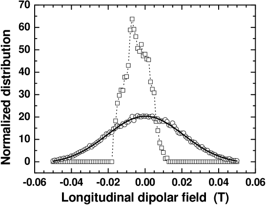
Fig. 3.10 : Calculated distribution of the longitudinal component $B_{\mathrm{dip}}^{(z)}$ of the dipolar fields in a ZFC (circles) and FC (squares) sample in zero external field. The solid line is a gaussian fit with width $2\sigma_{\mathrm{dip}}\simeq 0.042$ T, whereas the dotted line is just a guide for the eye (courtesy of I. S. Tupitsyn).

In a real sample consisting of a lattice of identical clusters, each molecule is also subject to the dipolar field $\vec{B}_{\mathrm{dip}}$ created by its neighbors, which adds a term $-g\mu_{B}\vec{S}\cdot\vec{B}_{\mathrm{dip}}$ in the Hamiltonian. A numerical calculation of the statistical distribution of such dipolar fields has been performed by I. S. Tupitsyn (Kurchatov Institute Moscow, Russia) by taking a “real” $40\times 40\times 40$ lattice of Mn₁₂-ac molecules, and assuming a certain value of the total magnetization. Fig. 3.10 shows the distribution of the longitudinal component $B_{\mathrm{dip}}^{(z)}$ of the dipolar fields in the case of a fully polarized, field-cooled (FC) sample and a demagnetized, zero-field cooled (ZFC) sample. Whereas the FC distribution is asymmetric and obviously depends on the size and shape of the crystal, the ZFC distribution can be well approximated by a gaussian with width $2\sigma_{\mathrm{dip}}\simeq 0.042$ T. In practice, this means that the vast majority of clusters is subject to a longitudinal bias $\xi\sim 0.1$ K, several orders of magnitude greater than the tunneling splitting; diagonalizing the Hamiltonian (3.14) including $\vec{B}_{\mathrm{dip}}$ yields indeed $S=10$, as argued on basis of the observed hyperfine fields. Nevertheless, there remains the possibility to reduce the total spin to less than 10 by applying a perpendicular field strong enough to produce a tunneling splitting larger than the dipolar bias. The exact way in which $\Delta$ becomes greater than $\xi$ is a delicate problem that must be solved by self-consistent numerical iteration, because as soon as some molecules have a small enough bias to cause the spin to reduce from 10 to $\langle S_{x}\rangle$, also the dipolar field they produce on their neighbors will suddenly be reduced, causing a drop in the width of the distribution of dipolar biases. Fig. 3.11(a) shows the full width $2\sigma_{\mathrm{dip}}$ of the distribution of longitudinal dipolar fields, calculated self-consistently on the real Mn₁₂-ac lattice and expressed in millitesla.

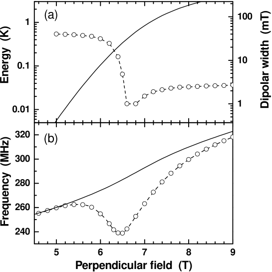
Fig. 3.11 : (a) Perpendicular field dependence of the full width $2\sigma_{\mathrm{dip}}$ of the longitudinal dipolar field distribution (circles), compared to that of the tunneling splitting $\Delta$ (solid line). (b) Calculated NMR spectra for the Mn⁽¹⁾ site as a function of perpendicular field. Solid line: calculated from (3.18, taking $S=10$ and independent of $B_{\perp}$ . Circles: calculated from (3.21), with $S(B_{\perp})$ as obtained by averaging over the dipolar fields distribution (courtesy of I. S. Tupitsyn).

Since we are interested in the consequences of such a phenomenon for the ⁵⁵Mn NMR spectrum, we first calculated numerically the values of $\langle S_{z}\rangle$ and $\langle S_{x}\rangle$ as function of $B_{x}$ by averaging over the self-consistently calculated distribution of dipolar biases. We then recalculated the total hyperfine field in Mn⁽¹⁾ sites by substituting

$$\tan\theta=\frac{\langle S_{x}\rangle}{\langle S_{z}\rangle}$$

$$B_{\mathrm{hyp}}(B_{x})=B_{\mathrm{hyp}}(0)\frac{\sqrt{\langle S_{x}\rangle^{2}+\langle S_{z}\rangle^{2}}}{10}$$ (3.21)

into Eq. (3.18). The resulting Larmor frequency is plotted in Fig. 3.11(b) and compared with the frequency that would be obtained assuming a constant value of $B_{\mathrm{hyp}}$, i.e. a constant total spin $S=10$. It clearly appears that the deviation from the $S=10$ spectrum occurs when $\Delta$ approaches the width of the dipolar field distribution. An actual observation of such a peculiar spectrum would imply that the total electron spin of the cluster is occupying a ground state consisting of a superposition of macroscopically distinct states for a time longer than the intrinsic NMR timescale, and that such a superposition of states is robust enough to survive the interaction with the environment and the measurement performed via the nuclear spins. To be completely correct, one should include the hyperfine interaction $\sum_{i}\vec{I}_{i}\cdot\mathbf{A}_{i}\cdot\vec{s}_{i}$ in the Hamiltonian (3.14) and solve the complete problem, but the size of the matrices would become intractable. We notice anyway that the hyperfine interactions are of the same order of magnitude as the dipolar fields, thus we can empirically assume that their effect on the localization of the electron spins should not be much larger than what we calculated so far by considering only $B_{\mathrm{dip}}$.

3.5 Nuclear spin dynamics

3.5.1 Nuclear spin-lattice relaxation (NSLR)

The general theory of nuclear relaxation, which expresses the spin-lattice relaxation rate as a function of the time correlation of a perturbing field[91], has been successfully applied to interpret the temperature dependence of the NSLR rate in the thermally activated regime of molecular magnets, first with proton NMR in Fe₈[92, 93, 94] and more recently with ⁵⁵Mn in Mn₁₂-ac[89, 95, 96]. We shall briefly review it here, mainly to point out why it breaks down upon approaching the pure quantum regime for the electron spin fluctuations. The implicit assumption that has always been made[92, 93, 94, 89, 95, 96] is that the nuclear spins have a certain Zeeman splitting, thus a certain Larmor frequency $\omega_{N}$, given by a static magnetic field, and that the transitions between the Zeeman levels of the static Hamiltonian can be computed within perturbation theory, assuming the presence of fluctuations in the hyperfine field which are small compared to the static field. In most cases, as in the ¹H experiments on Mn₁₂-ac [92, 93] (with the exception of [94]), the static field is an externally applied field, much larger than the hyperfine fields. For ⁵⁵Mn in Mn₁₂-ac however, the reverse is true and one may carry out an NMR experiment exploiting the local hyperfine field alone, which is made “quasi-static” by the high anisotropy barrier for the reversal of the electron spins. Thus, in the absence of an external field, the static field is just the value of $B_{\mathrm{hyp}}$ obtained when the electron spin is in its ground state. Fluctuations of the local field may then arise when the cluster spin is thermally excited to a higher level. Calling $b(t)$ the fluctuating component of $B_{\mathrm{hyp}}$, the NSLR rate $W$ can still be computed within the framework of perturbation theory if $b\ll B_{\mathrm{hyp}}$. $W$ is proportional to the spectral density at the Larmor frequency of the perpendicular component $b_{\perp}(t)$ of the fluctuating field, i.e. the Fourier transform of the time correlation function, $\langle b_{\perp}(t)b_{\perp}(0)\rangle$:

$$W=\frac{\gamma_{N}^{2}}{4}\int\langle b_{\perp}(t)b_{\perp}(0)\rangle\exp(i\omega_{N}t)dt.$$ (3.22)

We may further assume that the correlation function of $b_{\perp}(t)$ is related to the phonon-induced fluctuation rate $\tau_{\mathrm{s-ph}}^{-1}$ of the cluster electron spin as:

$$\langle b_{\perp}(t)b_{\perp}(0)\rangle=\langle\Delta b_{\perp}^{2}\rangle\exp(-t/\tau_{\mathrm{s-ph}}).$$ (3.23)

Here $\langle\Delta b_{\perp}^{2}\rangle$ is the square of the average change in the perpendicular component of the hyperfine field when the electron spin state is excited from $m=\pm 10$ to $m=\pm 9$. The spin-phonon transition rate $\tau_{\mathrm{s-ph}}^{-1}$ depends on the lifetime, $\tau_{9}$, and the activation energy, $\Delta E=E_{9}-E_{10}$, of the $m=\pm 9$ states as $\tau_{\mathrm{s-ph}}^{-1}=\tau_{9}^{-1}\exp(-\Delta E/k_{B}T)$, where:

$$\frac{1}{\tau_{9}}=\frac{C_{\mathrm{s-ph}}\Delta E^{3}}{1-\exp(-\Delta E/k_{B}T)}.$$ (3.24)

$\tau_{9}$ incorporates therefore the spin-phonon coupling constant $C_{\mathrm{s-ph}}$ [63, 67]. For the purpose of the present discussion we may neglect the higher lying levels, $|m|\geq 8$, which is a reasonable approximation below $T\sim 3$ K since $\Delta E>10$ K. Inserting into Eq. (3.22) we find:

$$W=\frac{\gamma_{N}^{2}}{4}\langle\Delta b_{\perp}^{2}\rangle\frac{\tau_{s-ph}}{1+\omega_{N}^{2}\tau_{s-ph}^{2}}\approx\frac{\langle\Delta b_{\perp}^{2}\rangle}{4B_{\mathrm{tot}}^{2}}\tau_{9}^{-1}\exp\left(-\frac{\Delta E}{k_{B}T}\right),$$ (3.25)

which shows clearly the expected exponential temperature dependence of the NSLR rate, since $\tau_{9}\simeq const.$ for $k_{B}T\ll\Delta E$.

Eq. (3.25) has the same form as the expression used by Goto et al.[95], except that the latter authors insert the $T$-dependence into an effective fluctuating field, expressed as:

$$b_{\mathrm{eff}}=\Delta b_{\perp}\frac{\tau_{9}}{\tau_{10}},$$

$$\frac{1}{\tau_{10}}=\frac{C_{\mathrm{s-ph}}\Delta E^{3}}{\exp(\Delta E/k_{B}T)-1},$$ (3.26)

where $\tau_{10}$ is the lifetime of the $m=\pm 10$ states, which is exponentially $T$-dependent. Goto et al. also pointed out that, in order to obtain a transverse component of the fluctuating hyperfine field upon excitation of the electron spin from $m=\pm 10$ to $m=\pm 9$, the hyperfine coupling tensor $\mathbf{A}$ (3.16) must contain non-vanishing off-diagonal terms. Then we may write $b_{\perp}=-\delta s_{z}A_{xz}/(\gamma_{N}\hbar)$, where $\delta s_{z}$ is the change in the $z$ component of the electron spin in each single ion. As mentioned in §3.3.1, only ⁵⁵Mn nuclei in Mn³⁺ have $A_{xz}\neq 0$ [87, 95], while $\mathbf{A}$ in Mn⁴⁺ sites is a diagonal tensor. We shall come back to the implications of this remark in §4.2.1 and §4.2.4.

As will become clear from the experiments presented in §4.2, although Eq. (3.25) properly fits the data in the thermally activated regime, it fails completely in the quantum regime ($T<0.8$ K), where the NSLR is found to become nearly independent of temperature. This phenomenon is observed in both the proton-NMR experiments in Fe₈ [94] and in our ⁵⁵Mn-NMR results, and clearly calls for a different theoretical approach. As will be further argued in §4.2, the NSLR in the quantum regime can be ascribed to the hyperfine field fluctuations arising from incoherent quantum tunneling of the electron spin between the $|+10\rangle$ and $|-10\rangle$ states. In this context, the crucial point is that the complete hyperfine field acting on the ⁵⁵Mn nuclei in a certain molecule will be suddenly inverted when the electron spin of that molecule tunnels, and will stay like that until the next tunneling event occurs. This means that a formalism such as that leading to Eq. (3.25) is unsuitable for describing the ⁵⁵Mn relaxation produced by tunneling events, because the effect of tunneling cannot be treated as a perturbation on a static Hamiltonian. As discussed in §3.2.3, the inversion of the hyperfine field takes place in a time $\tau_{\mathrm{tr}}\sim 10^{-12}$ s, i.e. instantaneous compared to $\omega_{N}^{-1}\sim 10^{-9}$ s, whereas the interval $\tau_{\mathrm{T}}$ between tunneling events is, as we shall show below, very long compared to the NMR window. The description of the nuclear spin dynamics in the presence of incoherent tunneling requires therefore a completely different approach, for which the basis has been laid by the Prokof’ev-Stamp theory[14], which we shall review in §3.6.

3.5.2 Transverse spin-spin relaxation (TSSR)

Another essential aspect of the nuclear spin dynamics is the transverse spin-spin relaxation (TSSR). Under the same hypotheses as for the NSLR, Goto et al.[95] have derived an expression for the TSSR rate $T_{2}^{-1}$ for the ⁵⁵Mn, that is applicable in the thermally activated regime of Mn₁₂-ac:

$$T_{2}^{-1}=\frac{1}{\tau_{10}}\times\frac{(\gamma_{N}\Delta b_{z}\tau_{9})^{2}}{1+(\gamma_{N}\Delta b_{z}\tau_{9})^{2}},$$ (3.27)

where $\Delta b_{z}$ is the change in longitudinal hyperfine field whenever the electron spin makes a transition between $m=\pm 10$ and $m=\pm 9$. In this approach the temperature dependence is incorporated in the lifetime $\tau_{10}$ of the $m=\pm 10$ states. Based on the analysis of the field-dependence of $T_{2}^{-1}$, they also conclude that the regime $(\gamma_{N}\Delta b_{z}\tau_{9})\gg 1$ holds, so that (3.27) becomes:

$$T_{2}^{-1}\approx\tau_{10}^{-1}=\frac{C_{\mathrm{s-ph}}\Delta E^{3}}{(\Delta E/k_{B}T)-1}.$$ (3.28)

In this model the decay of the transverse magnetization is basically due to a phase shift that occurs locally and randomly as a consequence of the sudden changes in the longitudinal component of the hyperfine hyperfine field (and thus in the Larmor frequency), for the nuclei in a thermally-excited cluster. In fact, this mechanism describes the dephasing of nuclear precession without considering any interaction between the nuclear spins.

The nuclear dipole-dipole interaction would add an extra contribution, whose magnitude can be calculated by taking into account the “flip-flop” term $\mathcal{H}_{f-f}$ in the dipolar Hamiltonian for two like spins $I^{(j)}$ and $I^{(k)}$ placed at a distance $r_{jk}$ and an angle $\theta_{jk}$ from each other [91]:

$$\mathcal{H}_{f-f}=-\frac{\hbar^{2}\gamma_{N}^{2}}{4r^{3}}(1-3\cos^{2}\theta_{jk})(I_{+}^{(j)}I_{-}^{(k)}+I_{-}^{(j)}I_{+}^{(k)}).$$ (3.29)

Using the Van Vleck formula one then obtains the contribution of the flip-flop term to the second moment $M_{2}$ of the resonance line, and the TSSR rate $T_{2}^{-1}$ as its square root:

$$M_{2}=\frac{1}{12}\gamma_{N}^{4}\hbar^{2}I(I+1)\sum_{k}\frac{(1-3\cos^{2}\theta_{jk})^{2}}{r_{jk}^{6}},$$

$$T_{2}^{-1}=\sqrt{M_{2}}.$$ (3.30)

Applying this formula to, for instance, the nuclei in Mn⁽¹⁾ sites, gives $T_{2}^{-1}=1790$ s^-1 if the Mn⁽¹⁾ nuclei in the same cluster are included, whereas restricting the summation to nuclei in neighboring clusters leads to $T_{2}^{-1}=111$ s^-1. The latter value gives an order of magnitude of the rate of intercluster nuclear spin diffusion which, as we shall discuss below, is an essential addition to the Prokof’ev-Stamp theory needed to understand our experiments.

3.6 Prokof’ev-Stamp theory

The Prokof’ev- Stamp (PS) theory of the spin bath [97, 14, 15] presents a major step forward in understanding the quantum dynamics of a giant spin (in our case the cluster spin) coupled to a bath of environmental spins (here the nuclear spins). The starting point for its development was to recognize that, in several physical systems, the “oscillator bath” theory [98] cannot be applied, because the environmental degrees of freedom cannot be described as a set of non-interacting oscillators, and the couplings to the central spin are not weak. Initially[97, 14], the PS theory was developed for a single central spin. The short-time $\sqrt{t}$ law for the quantum relaxation of an ensemble of spins (namely SMMs) has been obtained by including the effect of intercluster dipolar coupling in the form of an effective (bias) field [99]. This section contains a review the essential aspects of the PS theory, with emphasis on the issues that will be necessary to interpret the experimental results presented chapter IV. Fig. 3.12 can be used as a visual guide through the ingredients necessary to arrive at the complete description of the problem.

3.6.1 Central spin + spin bath

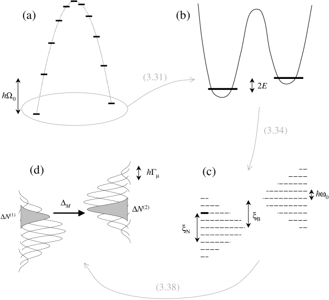
Fig. 3.12 : “Top-down” sketch of the model used by Prokof’ev and Stamp to describe the coupled system “central spin + spin bath”. The numbers in brackets indicate the equations that describe each further step. (a) Giant spin with crystal field anisotropy and external bias. (b) Truncation to the ground doublet, with static bias $\xi_{B}$. (c) Coupling with nuclear spins: this adds an extra bias $\xi_{N}$ which depends on the polarization state $\Delta N=N^{\uparrow}-N^{\downarrow}$ of the nuclei (cf. Fig. 3.14). (d) Nuclear spin diffusion: each polarization group is broadened by $\hbar\Gamma_{\mu}$, so that groups on either side of the barrier may overlap and create a tunneling window. Calling $\Delta N^{(1)}$ and $\Delta N^{(2)}$ the nuclear polarizations before and after the flip, the tunneling probability is governed by the effective tunneling splitting $\Delta_{M}$, with $2M=\Delta N^{(2)}-\Delta N^{(1)}$.

The first step for describing the coupled system of “central spin + spin bath” is to consider a single giant spin subject to crystal fields and, eventually, a magnetic field, and to truncate its total Hamiltonian to the ground doublet, neglecting all the physics at energies $>\Omega_{0}$ (see §3.2.3): in this way the central spin can be treated as an effective spin 1/2 described by Pauli matrices $\hat{\tau}$, where $|\Uparrow\rangle$ and $|\Downarrow\rangle$ are the eigenstates of $\hat{\tau}_{z}$. In particular, for an isolated spin having a tunneling splitting $\Delta$ in the ground doublet, the truncated Hamiltonian is:

$$\mathcal{H}_{\mathrm{trunc}}=\frac{\Delta}{2}\hat{\tau}_{x}\cos(\pi S)-\frac{\xi}{2}\hat{\tau}_{z},$$ (3.31)

where $\cos(\pi S)$ expresses the fact that in half-integer spins there is a destructive interference of tunneling paths [100, 101], and $\xi$ is a longitudinal bias. If such a bias is produced by an external static field, it is labelled $\xi_{B}=-2g\mu_{B}\vec{S}\cdot\vec{B}$. As is well known from textbook quantum mechanics [51], in the absence of any other couplings the probability $P_{\Uparrow\Uparrow}(t)$ for $\vec{S}$ to remain in the state $|\Uparrow\rangle$ at time $t$ when prepared in $|\Uparrow\rangle$ at $t=0$ is:

$$P_{\Uparrow\Uparrow}(t)=1-\frac{(\Delta/2)^{2}}{E^{2}}\sin^{2}(Et),$$ (3.32)

where $E=\sqrt{(\xi/2)^{2}+(\Delta/2)^{2}}$.

The central spin is further assumed to be coupled to $N$ environmental (e.g. nuclear) spins $\hat{\vec{\sigma}}_{k}$, $k=1\ldots N$, assumed for simplicity to have spin 1/2, described by vector Pauli matrices $\hat{\vec{\sigma}}_{k}$. In the notation of Prokof’ev and Stamp, the single hyperfine couplings have strength $\hbar\omega_{k}=\vec{\gamma}_{k}\cdot\vec{\sigma}_{k}$, where $\vec{\gamma}_{k}$ is the hyperfine field expressed in energy units, and they are centered around an average value $\hbar\omega_{0}$. The energy levels of the central spin are now represented by two hyperfine-split manifolds, each containing $2^{N}$ states distributed over a Gaussian with half-width $\sim\sqrt{N}\omega_{0}$. Degenerate states within the manifold can be labelled by their “polarization group”, i.e. according to the total nuclear polarization $\Delta N=N^{\uparrow}-N^{\downarrow}$ (see Fig. 3.14).

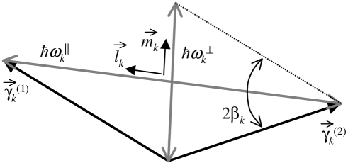
Fig. 3.13 : Scheme of the relative orientations of the hyperfine fields before ($\vec{\gamma}_{k}^{(1)}$) and after ($\vec{\gamma}_{k}^{(2)}$) the electron spin flip, and the consequent sum ($\hbar\omega_{k}^{\parallel}$) and difference ($\hbar\omega_{k}^{\perp}$) terms in the hyperfine energies, as defined in Eq. (3.33). The angle $\beta_{k}$ is typically very small since $\omega_{k}^{\parallel}\gg\omega_{k}^{\perp}$.

By calling $\vec{\gamma}_{k}^{(1)}$ and $\vec{\gamma}_{k}^{(2)}$ the hyperfine fields before and after the tunneling of the central spin, respectively, we can define the sum and difference terms:

$$\hbar\omega_{k}^{\parallel}\vec{l}_{k}=\vec{\gamma}_{k}^{(1)}-\vec{\gamma}_{k}^{(2)}$$

$$\hbar\omega_{k}^{\perp}\vec{m}_{k}=\vec{\gamma}_{k}^{(1)}+\vec{\gamma}_{k}^{(2)}$$ (3.33)

where $\vec{l}_{k}$ and $\vec{m}_{k}$ are unit vectors (cf. Fig. 3.13). $\hbar\omega_{k}^{\perp}$ represents the component of the hyperfine coupling energy that does not change during a flip of the central spin, whereas $\hbar\omega_{k}^{\parallel}$ is the variable part. For instance, in the case of ⁵⁵Mn nuclei in Mn₁₂-ac, one would find $\omega_{k}^{\perp}\approx 0$ since the hyperfine fields acting on $\vec{\sigma}_{k}$ before and after the flip are just antiparallel and equal in magnitude. These terms add a static (Zeeman) contribution to the Hamiltonian of the coupled system:

$$\mathcal{H}_{\mathrm{static}}=\frac{\hbar}{2}\left(\hat{\tau}_{z}\sum_{k}\omega_{k}^{\parallel}\vec{l}_{k}\cdot\hat{\vec{\sigma}}_{k}+\sum_{k}\omega_{k}^{\perp}\vec{m}_{k}\cdot\hat{\vec{\sigma}}_{k}\right).$$ (3.34)

The first term is a longitudinal coupling that yields an internal field bias acting on $\vec{\tau}_{z}$ that depends on the nuclear polarization, yielding a hyperfine bias $\xi_{N}=\hbar\omega_{0}\Delta N$ (see Fig. 3.14). Formally it plays the same role as $\xi_{B}$ discussed above, with the crucial difference that $\xi_{N}$ may vary in time, as we shall see below. The second term causes the so-called “orthogonality blocking”, since when $\vec{\gamma}_{k}^{(1)}\neq-\vec{\gamma}_{k}^{(2)}$, the basis for the eigenstates of $\vec{\sigma_{k}}$ (defined taking the quantization axis parallel to the instantaneous local field direction) after the flip of $\vec{S}$ is not exactly orthogonal to the basis before the flip. This means that after the flip $\vec{\sigma_{k}}$ will start to precess around a different axis, which quantum mechanically is equivalent to a transition between different nuclear Zeeman levels. The number of nuclear spins that would coflip by this mechanism is given by the parameter $\kappa$, defined as (cf. Fig. 3.13 for $\beta_{k}$):

$$e^{-\kappa}=\prod_{k}\cos\beta_{k}\approx e^{-\frac{1}{2}\sum_{k}\beta_{k}^{2}},$$

$$\cos(2\beta_{k})=\frac{-\vec{\gamma}_{k}^{(1)}\cdot\vec{\gamma}_{k}^{(2)}}{|\gamma_{k}^{(1)}||\gamma_{k}^{(2)}|}.$$ (3.35)

Clearly, $\kappa$ depends only on the direction of the hyperfine fields, and not on the timescale of the central spin flip.

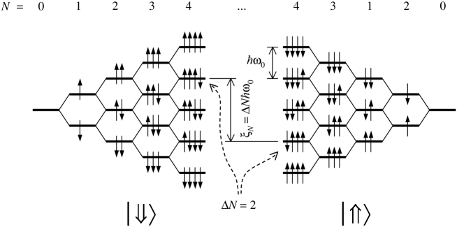
Fig. 3.14 : Sketch of the hyperfine-split manifold obtained by coupling the central spin to $N$ nuclear spins, with $N=1,2,\ldots$, assuming that all spins have $I=1/2$ and Zeeman splitting $\hbar\omega_{0}$. Notice how the bias $\xi_{N}=\hbar\omega_{0}\Delta N$ on the electron spin levels depends on the nuclear polarization $\Delta N$. This picture is valid only when all the nuclei have the same $\omega_{0}$; in a realistic case, the spread in hyperfine coupling makes the energy level scheme much more intricate.

Furthermore, the presence of environmental spins adds extra Berry phase terms to the $\cos(\pi S)$ discussed above, leading to the so-called “topological decoherence”. The detailed derivation of the total phase is not essential here, but we mention that it contains terms like $\alpha_{k}=(\pi/2)\omega_{k}/\Omega_{0}$, which depend on the ratio between the nuclear Larmor frequencies and the bounce frequency of the central spin (cf. §3.2.3). $\alpha_{k}^{2}$ is the probability for $\vec{\sigma}_{k}$ to coflip with $\vec{S}$ (see also [102]), but now for a different reason than the orthogonality blocking. What matters here is only the timescale of the flip compared to the period of Larmor precession, i.e. whether or not the nuclei can adiabatically follow the rotation of $\vec{S}$. A parameter

$$\lambda=1/2\sum_{k}\alpha_{k}^{2}$$ (3.36)

is introduced, that represents that number of nuclear spins that coflip with $\vec{S}$ because of the topological decoherence mechanism alone.

An additional aspect that must be included for a realistic description is the “degeneracy blocking”, which consists in allowing the hyperfine couplings to have a spread $\hbar\delta\omega_{k}$ around the central value $\hbar\omega_{0}$. This spread can have different origins (quadrupolar splitting, nuclear dipole-dipole interaction, transfer hyperfine interactions, Nakamura-Suhl interactions [103], etc.) and could potentially block the tunneling dynamics of the electron spin, since it breaks the degeneracy of the hyperfine-split electron spin states within the same polarization group. Because of the spread of nuclear frequencies, each polarization group is no longer represented by a sharp line, but rather by a Gaussian peak of width

$$\Gamma_{\mu}=\sqrt{N}\delta\omega_{k}.$$ (3.37)

In most cases, the gap between unperturbed polarization groups is much smaller than $\Gamma_{\mu}$, so that different polarization groups are in fact largely overlapping.

Because of the mutual dipolar coupling between nuclear spins:

$$\mathcal{H}_{\mathrm{dip}}(\{\sigma_{k}\})=\sum_{k\neq k^{\prime}}V_{kk^{\prime}}^{\alpha\beta}\hat{\sigma}_{k}^{\alpha}\hat{\sigma}_{k^{\prime}}^{\beta},$$ (3.38)

there is an intrinsic broadening $\delta\omega_{k}^{(\mathrm{dip})}\sim T_{2}^{-1}$ of the nuclear Zeeman levels. The crucial point is to recognize that this broadening is dynamic, due to nuclear spin diffusion. In practice, the hyperfine bias can fluctuate and cover the whole range of each polarization group, i.e. an amplitude $\hbar\Gamma_{\mu}$, on a timescale $\sim T_{2}$. The effect of spin diffusion is therefore to eliminate the degeneracy blocking. Notice that this sort of fluctuations arises from what one would call “intracluster” spin diffusion, since the model is written for one single central spin coupled to his nuclear spins. The transition between different polarization groups would therefore require the exchange of energy with an external reservoir, on a timescale $T_{1}$; in the PS theory, this mechanism is assumed to take very long times. On the other hand, by taking many identical “central spin + spin bath” units, one may allow for “intercluster” spin diffusion as well, i.e. between equivalent nuclei belonging to different clusters. This possibility is not explicitly discussed in the early PS papers, but will play an essential role in the interpretation of our experimental results.

3.6.2 Tunneling rate

The strategy adopted by Prokof’ev and Stamp to derive the incoherent tunneling rate of the central spin coupled to a spin bath, is to estimate it from the evolution of the probability $P_{\Uparrow\Uparrow}(t)$ for $\vec{S}$ to remain in the same state $|\Uparrow\rangle$ until time $t$. Its trivial expression for an isolated spin is Eq. (3.32); including the spin bath one has to average over the different values $P_{M}(t)$ that $P_{\Uparrow\Uparrow}(t)$ may take, depending on the change $2M$ of the polarization state $\Delta N=N^{\uparrow}-N^{\downarrow}$ of the environmental spins caused by the flip of $\vec{S}$. $P_{M}(t)$ is itself obtained by averaging, over the “topological” and “orthogonality blocked” processes, the quantity $P_{M}^{(0)}(t)$, defined as:

$$P_{M}^{(0)}(t)=1-\frac{(\Delta_{M}/2)^{2}}{E_{M}^{2}}\sin^{2}(E_{M}t)$$ (3.39)

$$E_{M}^{2}=(\xi/2)^{2}+(\Delta_{M}/2)^{2}$$ (3.40)

$$\Delta_{M}\sim\Delta_{0}\frac{(\lambda-\lambda^{\prime})^{M/2}}{M!},$$ (3.41)

where $\lambda^{\prime}=\lambda$ in the case of pure topological decoherence and $\lambda^{\prime}=0$ for pure orthogonality blocking, and for $\xi$ we take the total bias $\xi=\xi_{N}+\xi_{B}$ which may include the effect of an externally applied field. Roughly speaking, this means that the effect of the spin bath is incorporated in a renormalization of the tunneling splitting, assigning a vanishingly small value of $\Delta_{M}$ to those tunneling transitions that would require too many nuclear coflips, as compared to the “natural values” of $\kappa$ and $\lambda$. The really essential point is that $\xi$ in Eq. (3.40) is no longer a static bias, as soon as nuclear spin diffusion is allowed. From (3.38) one finds that $\xi_{N}$ contains a time-dependent part which fluctuates on a timescale $T_{2}^{-1}$ over a range $\sim\hbar\Gamma_{\mu}$, which is the change in longitudinal hyperfine bias when $N$ pairwise $|\uparrow\downarrow\rangle\rightarrow|\downarrow\uparrow\rangle$ nuclear flip-flops occur. With the assumption that $T_{2}$ is much shorter than the typical tunneling interval $\tau_{T}$, the average of $P_{M}^{(0)}(t)$ over the fluctuating bias can be written as:

$$\langle P_{M}^{(0)}(t,\xi)\rangle_{\xi}-\frac{1}{2}=\frac{1}{2}e^{-t/\tau_{M}}$$ (3.42)

$$\tau_{M}^{-1}=\frac{\Delta_{M}^{2}}{2\sqrt{\pi}\hbar^{2}\Gamma_{\mu}}.$$ (3.43)

The parameter $\tau_{M}^{-1}$ represents therefore the rate for $\vec{S}$ to tunnel accompanied by the coflip of $M$ nuclear spins. In the presence of an external static bias $\xi_{B}$, $\tau_{M}^{-1}$ starts to be suppressed as soon as $\xi_{B}$ is larger than the typical hyperfine field spread. Combining this with the fact that the largest tunneling splitting is obtained for $M=0$, one finds that the leading term in the tunneling rate takes the form:

$$\tau^{-1}=\frac{\Delta_{0}^{2}}{2\sqrt{\pi}\hbar^{2}\Gamma_{\mu}}e^{-|\xi_{B}|/\xi_{0}}.$$ (3.44)

where $\xi_{0}$ is the width of the “tunneling window”. When some nuclear spins may coflip with $\vec{S}$ by topological decoherence ($\lambda$) or orthogonality blocking ($\kappa$), then $\xi_{0}$ is given by the energy that the central spin can exchange with the nuclear spin bath, $\xi_{0}\sim(\lambda+\kappa)\hbar\omega_{0}$. Otherwise, in the absence of nuclear coflips the tunneling window takes the width $\xi_{0}\sim\hbar\Gamma_{\mu}$ due to nuclear spin diffusion only. From this discussion it is clear that the major role in creating a useful tunneling window for the central spin is played by those nuclei that more easily coflip with $\vec{S}$. We anticipate that this is an experimentally testable prediction (§4.2.3).

The global relaxation, i.e. the precise form of $P_{\Uparrow\Uparrow}(t)$, is obtained by combining all the results discussed above. This leads to very interesting phenomena to be observed in the quantum relaxation, but goes beyond the scope of our research. We shall mainly make use of the tunneling rates (3.43),(3.44) and the concepts of topological decoherence and orthogonality blocking to evaluate the numbers of coflipping nuclei $\lambda$ and $\kappa$.

3.6.3 Comparison with the Landau-Zener formalism

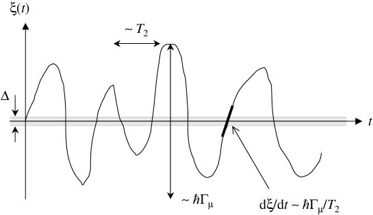
Fig. 3.15 : Time evolution of the bias $\xi$ on the central spin levels as a consequence of nuclear spin diffusion: the crossing through the tunneling resonance happens with slope $\mathrm{d}\xi/\mathrm{d}t\sim\hbar\Gamma_{\mu}/T_{2}$.

It is rather instructive to compare the Prokof’ev-Stamp theory with the Landau-Zener formula (3.11) for the calculation of an incoherent tunneling rate. In the presence of nuclear spin diffusion, assuming for simplicity the external bias $\xi_{B}=0$, the bias $\xi$ fluctuates over a range $\hbar\Gamma_{\mu}$ on a timescale $T_{2}$, thereby forcing the energy levels of the central spin $\vec{S}$ to cross back and forth through the tunneling resonance: a sketch of the situation is given in Fig. 3.15. We could therefore think of applying Eq. (3.11), simplified by noting that $\Delta^{2}$ is a very small number and expanding the exponential:

$$P_{LZ}\approx\frac{\pi\Delta^{2}}{2\hbar}\left(\frac{\mathrm{d}\xi}{\mathrm{d}t}\right)^{-1}.$$ (3.45)

Clearly, in our case $\mathrm{d}\xi/\mathrm{d}t\sim\hbar\Gamma_{\mu}/T_{2}$, yielding $P_{LZ}\sim(\Delta^{2}/\hbar)[(T_{2}/(\hbar\Gamma_{\mu})]$. To obtain the tunneling rate, we multiply the single tunneling probability by the number of crossings per unit time, i.e. $T_{2}^{-1}$, and obtain

$$\tau_{LZ}^{-1}\sim\frac{\Delta^{2}}{\hbar^{2}\Gamma_{\mu}},$$ (3.46)

which has indeed the same form as Eq. (3.43). Deriving it via the LZ formalism clarifies why the tunneling rate does not contain the timescale $T_{2}$ of the bias fluctuations. On the other hand, by this we have completely lost any information about the effect of the central spin dynamics on its nuclei, which in Eq. (3.43) is incorporated in the renormalized tunneling splitting $\Delta_{M}$, cf. (3.41). An essential feature of the PS theory is indeed that the fluctuating bias is not added artificially as an “environmental noise”, uncorrelated with the dynamics of $\vec{S}$, but is built in the model in a self-consistent way, including the back-action of $\vec{S}$ on the nuclear spins [104].

3.6.4 Application to SMMs

When applying the PS theory to the combined electron-nuclear spin dynamics in SMMs, it is useful to distinguish between nuclei coupled directly to one single ion, like ⁵⁵Mn in Mn₁₂-ac, and nuclei located at the ligand molecules, like ¹H (and a small fraction of ¹³C). In the latter case, the strength of the coupling is of course much lower than for ⁵⁵Mn, since it is due mainly to dipolar fields, but the total field is the sum of the dipolar fields from different molecules. If one molecule flips, it is only one component of the total field at the ¹H site that flips, which may yield a situation where $\beta_{k}$, and therefore the chance of nuclear coflip, is rather large (cf. Fig. 3.8). This means that the protons can be the main contributors to the width of the tunneling window $\xi_{0}$, despite the relatively weak coupling.

On the contrary, $\beta_{k}\simeq 0$ in ⁵⁵Mn, since the whole hyperfine field is inverted by $180^{\circ}$ upon tunneling. This yields $\kappa\simeq 0$ and, because of the short tunneling traversal time (cf. §3.2.3), $\lambda\simeq 0$ as well. Clearly, we can expect the change of polarization group for ⁵⁵Mn nuclei to be very difficult, unless nuclei in different clusters are linked with each other. This possibility is not explicitly discussed in the PS theory, but we shall see in the next chapter that it is both experimentally observed (§4.2.1), and necessary to explain the observed ⁵⁵Mn NSLR rate in Mn₁₂-ac.

Chapter 4 Nuclear spin dynamics in Mn₁₂-ac

The nuclear spin dynamics in a single-molecule magnet is one of the most crucial aspects influencing its quantum behavior, nonetheless the experimental knowledge was so far almost totally lacking, in particular in the low-$T$ quantum regime for the cluster spin fluctuations. We dedicate therefore this chapter to a detailed survey of our results on the ⁵⁵Mn NMR in Mn₁₂-ac, starting with the temperature dependence of the nuclear spin-lattice relaxation (NSLR) and transverse spin-spin relaxation rates (TSSR) in zero external field. The data indicate that quantum tunneling of the electron spin is the mechanism responsible for the observed features in the nuclear spin dynamics. The dependencies on small longitudinal fields, magnetization state of the electron spins, isotope substitution, and crystallographic Mn site, yield precious additional information. We then discuss the influence on the NSLR of an external perpendicular field, which can be used to tune the tunneling splitting. Finally, an essential and original information is provided by the study of the nuclear spin temperature. The results are very surprising and call for an extension of the existing theory of quantum tunneling in magnetic molecules. The chapter is concluded by a suggestion for an approach that should unify all the experimental evidences into a new and more complete theoretical description.

4.1 Measurements and data analysis

About 100 mg of Mn₁₂-ac crystallites were mixed with Stycast 1266 epoxy and introduced into a $\varnothing$ $6$ mm capsule, then inserted in the room-temperature bore of a 9.4 T magnet and allowed to orient for 24 hours. A two-turns NMR coil was wound around the capsule, the whole assembly was inserted inside the mixing chamber of the dilution refrigerator (§2.1) and connected to the NMR electronics as described in §2.2.2.

The ⁵⁵Mn nuclear precession was detected by the spin-echo technique. A typical pulse sequence includes a first $\pi/2$-pulse with duration $t_{\pi/2}=12$ $\mu$s, a waiting interval of 45 $\mu$s, and a 24 $\mu$s $\pi$-pulse for refocusing. At the lowest temperatures provided by the dilution refrigerator, such a pulse sequence was found to cause an increase in temperature of about 5 mK in the ³He/⁴He mixture. With a waiting time of 600 s between subsequent pulse trains we could easily keep the operating temperature around $15-20$ mK (cf. Fig. 2.5). On the other hand, at such low temperature the signal intensity is so high that we could obtain an excellent S/N ratio without need of averaging, so that a typical measurement sequence (e.g. an inversion recovery) would last less than 12 hours. Above 100 mK it proved convenient to take a few averages, but then the heating due to the rf-pulses becomes negligible, and the waiting time can be reduced to $\sim 100$ s.

Fig. 4.1 : An example of “real time” echo signals recorded during an inversion recovery, i.e. measuring the echo intensity at increasing delays after an inversion pulse. In particular, these are single-shot (no averaging) raw data taken at $B=0$ and $T=20$ mK in the Mn⁽¹⁾ site. The (normalized) integral of the echoes is reported in Fig. 4.2, open squares.

The NSLR was studied by measuring the recovery of the nuclear magnetization after an inversion pulse (cf. Fig. 2.3). We preferred this technique to the more widely-used saturation recovery [89, 87, 95] because it avoids the heating effects of the saturation pulse train, but we checked at intermediate temperatures that the two techniques indeed lead to the same value of NSLR rate. An example of echo signals obtained as a function of the waiting time after the inversion pulse is shown in Fig. 4.1. By integrating the echo intensity we obtained recovery curves such as those shown in Fig. 4.2. For the ease of comparison between different curves, we renormalize the vertical scale such that $M(0)/M(\infty)=-1$ and $M(t\gg T_{1})/M(\infty)=1$, even though usually $|M(0)|<|M(\infty)|$, as could be deduced from Fig. 4.1. Since the ⁵⁵Mn nuclei have spin $I=5/2$, the recovery of the nuclear relaxation for the central line in the quadrupolar split manifold is described by [105]:

$$\frac{M(t)}{M(\infty)}=1-\left[\frac{100}{63}e^{-30Wt}+\frac{16}{45}e^{-12Wt}+\frac{2}{35}e^{-2Wt}\right]$$ (4.1)

where $W$ is the nuclear spin-lattice relaxation rate. All data in zero field and moderate parallel fields could be accurately fitted by Eq. (4.1), which indicates that the relaxation mechanism can be characterized by a single rate $W$. Conversely, a proper analysis of the inversion recoveries in strong perpendicular fields requires the introduction of a stretching exponent $\alpha$:

$$\frac{M(t)}{M(\infty)}=1-\left[\frac{100}{63}e^{-(30Wt)^{\alpha}}+\frac{16}{45}e^{-(12Wt)^{\alpha}}+\frac{2}{35}e^{-(2Wt)^{\alpha}}\right]$$ (4.2)

This can be attributed to a small distribution of orientations of the crystallites in the sample, which causes the NMR signal in high fields to consist of a mixture of lines from different crystallites, each of them characterized by a different NSLR rate. A comparison between an inversion recovery at zero field, fitted by Eq. (4.1), and a similar recovery in strong perpendicular field fitted by Eq. (4.2), is shown in Fig. 4.2.

Fig. 4.2 : Examples of nuclear inversion recoveries in zero field (squares) and strong perpendicular field (circles). The NSLR rate $W$ is extracted by fitting the data with Eq. (4.1) or Eq. (4.2), respectively.

The TSSR rate $T_{2}^{-1}$ was studied by measuring the decay of echo intensity upon increasing the waiting time $\tau$ between the $\pi/2$- and the $\pi$-pulses. The decay of transverse magnetization $M_{\perp}(\tau)$ can be fitted by a single exponential

$$\frac{M_{\perp}(2\tau)}{M_{\perp}(0)}=\exp\left(-\frac{2\tau}{T_{2}}\right)$$ (4.3)

except at the lowest temperatures ($T\lesssim 0.2$ K), where also a gaussian component $T_{2G}^{-1}$ needs to be included:

$$\frac{M_{\perp}(2\tau)}{M_{\perp}(0)}=\exp\left(-\frac{2\tau}{T_{2}}\right)\exp\left(-\frac{(2\tau)^{2}}{2T_{2G}^{2}}\right)$$ (4.4)

As regards the experiments to determine the nuclear spin temperature, the measurements were performed by monitoring the echo intensity at regular intervals while changing the temperature $T_{\mathrm{bath}}$ of the ³He/⁴He bath in which the sample is immersed. Recalling (§2.2.1) that nuclear magnetization is related to the nuclear spin temperature $T_{\mathrm{nucl}}$ by the Curie law:

$$M(T_{\mathrm{nucl}})=N\frac{\gamma_{N}^{2}\hbar^{2}I(I+1)}{3k_{\mathrm{B}}T_{\mathrm{nucl}}},$$ (4.5)

and assuming that $T_{\mathrm{bath}}=T_{\mathrm{nucl}}$ at a certain temperature $T_{0}$ (e.g. 0.8 K), we can define a calibration factor $K$ such that $M(T_{0})=K/T_{\mathrm{nucl}}(T_{0})$ and use that definition to derive the time evolution of the nuclear spin temperature as $T_{\mathrm{nucl}}(t)=K/M(t)$ while the bath temperature is changed.

4.2 Nuclear relaxation in moderate parallel fields

In this section we present and discuss the experimental results on the ⁵⁵Mn spin-lattice and spin-spin relaxation rates in Mn₁₂-ac, starting with the temperature dependencies in zero field, and then discussing the effect of small longitudinal fields and isotope substitution. All data refer to Mn⁽¹⁾ sites, except for §4.2.4, where a comparison with the Mn⁽²⁾ site is presented.

4.2.1 NSLR and TSSR in zero field

As mentioned in §3.5.1, the NSLR and TSSR in Mn₁₂-ac have already been studied in quite some detail in the thermally activated regime by other groups [89, 95, 96], whereas the purpose of our work has been to extend the analysis deep into the pure quantum regime [96]. We begin by discussing the temperature dependencies of the NSLR and TSSR rates in a demagnetized, zero-field-cooled (ZFC) sample, shown in Fig. 4.3.

What clearly appears is a sharp crossover at $T\simeq 0.8$ K between a roughly exponential $T$-dependence and an almost $T$-independent plateau. We attribute the $T$-independent nuclear relaxation to the effect of ground-state tunneling fluctuations of the cluster spins, and we shall dedicate most of this chapter to discuss our further results supporting this statement. It should be noted that the crossover from thermally activated to ground-state tunneling has been also observed by analyzing the $T$-dependence of the steps in the magnetization loops [106, 107]. The important advantage of our NMR measurements is that the nuclear dynamics is sensitive to fluctuations of the cluster electron spins without even requiring a change in the macroscopic magnetization of the sample. Clearly, no macroscopic probe (except perhaps an extremely sensitive magnetic noise detector) would be able to detect the presence of tunneling fluctuations in a zero-field cooled sample in zero external field, since the total magnetization is zero and remains so. In fact, below $T\sim 1.5$ K the steps in the hysteresis loops of Mn₁₂-ac can be observed only at relatively high values of external field [106, 107], which is indeed predicted to lead to a less sharp transition between thermally activated and quantum regimes [108]. We fitted the high-$T$ part of the NSLR rate by Eq. (3.25), as shown by the dotted line in Fig. 4.3: the curve depicted is obtained by fixing $\Delta E=D(10^{2}-9^{2})+B_{4}(10^{4}-9^{4})=14.4$ K which yields $\langle\Delta b_{\perp}^{2}\rangle/\tau_{9}\simeq 1.1\times 10^{7}$ T² s^-1. The fit, in particular its slope, may be improved by leaving also $\Delta E$ as a free parameter, which then yields $\Delta E\simeq 12.2$ K and $\langle\Delta b_{\perp}^{2}\rangle/\tau_{9}\simeq 2.2\times 10^{6}$ T² s^-1. Despite the reasonable quality of the fit, Eq. (3.25) is based on a model which is seriously questionable for two reasons: (i) it considers only hyperfine field fluctuation due to “intrawell” excitation, i.e. it does not account for thermally-assisted tunneling through excited doublets, and (ii) it does not explain what is the source of transverse fluctuating field $b_{\perp}$, since the hyperfine coupling tensor in Mn⁴⁺ does not contain non-diagonal elements (cf. §3.5.1). We may already notice that including “interwell” fluctuations due to thermally assisted tunneling could solve the paradox of the transverse hyperfine field component, provided we can demonstrate that quantum tunneling of the electron spin is a possible source of nuclear relaxation. We shall come back to this issue in §4.2.4.

The roughly $T$-independent plateau in the NSLR rate below $T\simeq 0.8$ K is characterized by a value of $W\simeq 0.03$ s^-1 that is surprisingly high, which at first sight may appear like an argument against the interpretation in terms of tunneling fluctuations of the electron spin. Experimentally it is indeed well known [109] that the relaxation of the magnetization in Mn₁₂-ac in zero field may take years at low $T$, which means that the tunneling events are in fact extremely rare. Based on this, we are forced to assume that the tunneling events take place only in a small minority of the clusters, and that some additional mechanism takes care of the relaxation of the nuclei in molecules that do not tunnel. This is a very realistic assumption indeed, since it is well known that all samples of Mn₁₂-ac contain a fraction of fast-relaxing molecules (FRMs) [83, 82], as anticipated in §3.2.4. Moreover, that the tunneling dynamics has to be ascribed to FRMs is supported by the experimental fact that, when measuring the NSLR in zero field in a saturated field-cooled sample (FC), we observe that the sample magnetization does not change during the experiment. This can be done by applying a small longitudinal field $B_{z}\sim 0.5$ T and measuring the NMR signal intensity at the shifted frequencies $\nu_{\uparrow}=\nu(0)+\gamma_{N}B_{z}$ and $\nu_{\downarrow}=\nu(0)-\gamma_{N}B_{z}$, corresponding to nuclei in clusters whose spin is respectively parallel or antiparallel to the external field [110, 87]. In a fully saturated sample, the NMR signal at $\nu_{\downarrow}$ is indeed zero, and we verified that it remains that way even after several weeks of experiments as long as the sample is kept constantly at low temperature. In other words, the macroscopic magnetization as seen by the nuclei that contribute to the NMR signal does not change in time, implying that the observable NMR signal comes from nuclei that belong to “frozen” clusters, therefore the relaxation channel must involve the tunneling in FRMs.

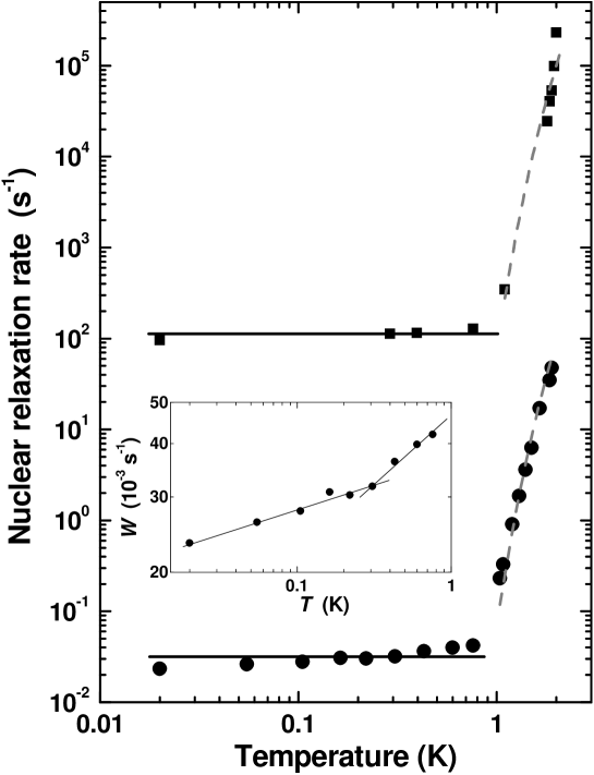
Fig. 4.3 : Temperature-dependence of the NSLR (circles) and TSSR (squares) rates for a ZFC sample in zero field and $\nu=231$ MHz. The dashed lines are fits to Eqs. (3.25) and (3.28), with parameters discussed in the text. The inset is an enlargement of $W(T)$ for $T<0.8$ K, with lines as guides for the eye.

The question remains what is the mechanism that links the tunneling in FRMs to the nuclear spins in frozen molecules. One possibility is to ascribe it to the fluctuating dipolar field produced by a tunneling FRM at the nuclear sites of neighboring frozen molecules. In that case we may give an estimate of $W$ using an expression of the form:

$$W\approx\frac{\gamma_{N}^{2}}{4}b_{\mathrm{dip}}^{2}\frac{\tau_{\mathrm{T}}}{1+\omega_{N}^{2}\tau_{\mathrm{T}}^{2}}\approx\frac{b_{\mathrm{dip}}^{2}}{4B_{\mathrm{tot}}}\tau_{\mathrm{T}}^{-1},$$ (4.6)

where $b_{\mathrm{dip}}$ is the perpendicular component of the fluctuating dipolar field produced by a tunneling molecule on its neighbors and $\tau_{\mathrm{T}}^{-1}$ is the tunneling rate. Even for nearest neighbors $b_{\mathrm{dip}}<3$ mT, which leads to the condition $W\simeq 0.03$ s^-1 $\Rightarrow\tau_{\mathrm{T}}\gg 10^{6}$ s^-1. This is completely unrealistic, even for the FRMs with two flipped Jahn-Teller axes. It is therefore unavoidable to consider the effect of a tunneling molecule on the nuclei that belong to the molecule itself, and to look for an additional mechanism that links nuclei in FRMs with equivalent nuclei in frozen clusters. It is natural to seek the origin of such a mechanism in the intercluster nuclear spin diffusion, and we shall provide strong experimental evidences to support such an interpretation.

By magnifying the NSLR rate in the quantum regime (inset of Fig. 4.3 we notice that the plateau is in fact not perfectly horizontal but seems to have two slopes, with most pronounced one for $T\gtrsim 0.3$ K. We may attribute this slope to the thermally-assisted intrawell fluctuations in the FRMs, i.e. the same phenomenon as observed for $T>0.8$ in the whole sample. Since the FRMs have a lower anisotropy and therefore lower $\Delta E$, we may expect their crossover from quantum to thermally activated regime to take place at a lower temperature. Magnetization measurements [82] have indicated that the crossover takes place at $T\simeq 0.6$ K in the FRMs with just one flipped Jahn-Teller axis, but this value could be of course lower for the FRMs with two flipped axis and 15 K barrier.

Fig. 4.3 also shows the $T$-dependence of the TSSR rate $T_{2}^{-1}(T)$. We observe that above 0.8 K $T_{2}^{-1}(T)$ has the same $T$-dependence as the NSLR rate, and can be fitted by Eq. (3.28) with $\Delta E=14.4$ K. This indicates that the fluctuations arising from thermal activation of the electron spin are responsible for the TSSR as well, at least in this temperature regime.

Below 0.8 K the TSSR also saturates to a nearly $T$-independent plateau. By fitting the decay of transverse magnetization with Eq. (4.3) at all temperatures we obtain $T_{2}^{-1}\simeq 100$ s^-1. This is just a rough estimate since, as mentioned in §4.1, the transverse relaxation is not well described by a single exponential decay below $T\lesssim 0.2$ K. Nevertheless, we find this estimate to be comparable with the value $T_{2}^{-1}=111$ s^-1 calculated on basis of the dipole-dipole coupling of nuclei in neighboring clusters (§3.5.2). It is of great interest to point out that in a ZFC sample, to which the data in Fig. 4.3 refer, only half of the nuclei in neighboring molecules should be taken into account as possible partners for flip-flop transitions. Since half of the cluster spins point up and the other half point down, the nuclear spins in equivalent sites should be split in two groups having Larmor frequencies $+\omega_{N}$ and $-\omega_{N}$, respectively. For the purpose of calculating the TSSR rate that results from intercluster nuclear spin diffusion, this is equivalent to having diluted the system by a factor 2. Carrying out the sum (3.30) over half of the spins only, reduces the calculated TSSR rate by a factor $\sqrt{2}$, yielding $T_{2}^{-1}=78$ s^-1 for a ZFC sample, whereas the above-mentioned $T_{2}^{-1}=111$ s^-1 remains the correct estimate for a FC sample. Moreover, the dipole-dipole coupling should lead to a roughly gaussian decay of the transverse nuclear magnetization [91].

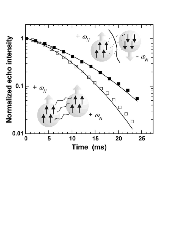
Fig. 4.4 : Decay of transverse nuclear magnetization in FC (open circles) and ZFC (full circles) sample at $T=20$ mK, zero applied field and $\nu=231$ MHz. The lines are fits to Eq. (4.4) yielding the ratio $T_{2G}^{-1}(\mathrm{FC})/T_{2G}^{-1}(\mathrm{ZFC})=1.35\simeq\sqrt{2}$. The inset sketches represent pictorially the fact that intercluster spin diffusion is possible in a FC sample since all the nuclei have the sam Larmor frequency, contrary to the case of a ZFC sample.

We have indeed been able to verify both these predictions by measuring the TSSR at $T=20$ mK in a FC and a ZFC sample, as shown in Fig. 4.4. The decay of the transverse magnetization is indeed best fitted by Eq. (4.4), whereby the Gaussian component, $T_{2G}^{-1}$, is separated from the Lorentzian one, $T_{2L}^{-1}$. From the Gaussian component of the decay we can extract directly the effect of the nuclear dipole-dipole interaction, whereas the other mechanisms of dephasing (e.g. random changes in the local field, cf. §3.5.2) contribute mainly to the Lorentzian part. The fit yields $T_{2G}^{-1}(\mathrm{FC})=104\pm 3$ s^-1 and $T_{2G}^{-1}(\mathrm{ZFC})=77\pm 3$ s^-1, respectively; the ratio $T_{2G}^{-1}(\mathrm{FC})/T_{2G}^{-1}(\mathrm{ZFC})=1.35$ of the TSSR rates in FC and ZFC samples agrees indeed with the prediction of a $\sqrt{2}$ reduction of the intercluster flip-flop rate in a ZFC sample and constitutes solid evidence for the presence of intercluster nuclear spin diffusion. This experimental finding points to the need of an extension of the basic assumption of the Prokof’ev-Stamp theory [14] to the case of an assembly of interacting “central spin - spin bath” units. It also supports our previous interpretation of the mechanism of nuclear spin-lattice relaxation in terms of the combined effect of tunneling in FRMs plus nuclear spin diffusion. We stress that, in view of our quantitative analysis of the TSSR, the fact that the NSLR and the TSSR are both roughly $T$-independent below 0.8 K does not mean that they have the same origin in this regime. Rather, we attribute them to two different mechanisms, both $T$-independent: the quantum tunneling of the electron spin (for the NSLR) and the nuclear spin diffusion (for the TSSR). It is only for $T>0.8$ that the same thermal fluctuations are responsible for NSLR and TSSR at the same time.

We point out that, in spite of the even quantitative agreement with the simple picture of intercluster nuclear spin diffusion as described by Eq. (3.30), a puzzling point remains. Due to the dipolar field produced by neighboring clusters, ⁵⁵Mn nuclei in different molecules will have different Zeeman energies, and the typical magnitude of the energy spread involved is actually much greater than the intercluster nuclear dipole-dipole coupling, and should lead to a strong suppression of the flip-flop probability. We shall suggest a solution to this problem in the next subsection, when discussing the field dependence of the TSSR rate.

4.2.2 Field dependencies

Further insight in the interplay between quantum tunneling and nuclear spin dynamics is provided by the study of the dependence of the NSLR and TSSR rates on a magnetic field $B_{z}$ applied along the anisotropy axis. It is clear from the Hamiltonian (3.14) that, in the absence of other perturbations, such a longitudinal field destroys the resonance condition for corresponding electron spin states on both sides of the barrier and therefore inhibits the quantum tunneling. In the presence of static dipolar fields, $B_{\mathrm{dip}}$, by studying the tunneling rate as a function of $B_{z}$ one may in principle obtain information about the distribution of longitudinal $B_{\mathrm{dip}}$, since at a given value of $B_{z}$ there will be a fraction of molecules for which $B_{\mathrm{dip}}=-B_{z}$ and will therefore be allowed to tunnel just by the application of the external bias. We measured the longitudinal field dependence of the NSLR rate $W(B_{z})$ while shifting the measuring frequency $\nu(B_{z})=\nu(0)+\gamma_{N}B_{z}$ with $\nu(0)=230$ MHz, in order to stay on the center of the NMR line that corresponds to the molecules that are aligned exactly parallel with the applied field.

The results for the ZFC sample at $T=20$ mK are shown in Fig. 4.5. Since for a ZFC sample the magnetization is zero, the field dependence should be the same when $B_{z}$ is applied in opposite directions, as is observed. The data can be fitted by a Lorentzian with a full width at half maximum $\Delta B_{z}=0.12$ T, thus different both in shape and in width from the calculated dipolar bias distribution (Fig. 3.10). A possible reason for the extra broadening observed in $W(B_{z})$ could be the presence of misaligned molecules in the sample, combined with quadrupolar broadening of the NMR line. The manifold of quadrupolar-split Mn⁽¹⁾ lines can be closely described as a gaussian with total width $2\sigma_{\nu}\simeq 2.4$ MHz, i.e. $\simeq 0.23$ T in field units, thus already broader than $W(B_{z})$. Although we follow the center of the line for the well-aligned molecules, the misaligned ones (which experience a smaller longitudinal field) could still be in condition to tunnel and contribute to the NMR signal by means of their quadrupolar satellite lines. An obvious source of misalignment is the fact that our sample consists of an ensemble of crystallites, thus there is the chance for part of them to be misoriented. In fact, the misalignment is in any case unavoidable for fast-relaxing molecules, which we consider to be the actual source of quantum tunneling events. It is known (cf. §3.2.4) that the FRMs with one flipped Jahn-Teller axis also have a local anisotropy axis for the cluster spin which deviates $\sim 10^{\circ}$ from the crystallographic $\hat{c}$-axis, and the misalignment could be even greater for the FRMs with two flipped J-T axes. A confirmation for the role of misaligned molecules in the width of $W(B_{z})$ comes from the fact that, if we repeat the experiment taking $\nu(0)=231$ MHz, thus slightly higher than the center of the line, $W(B_{z})$ appears indeed much narrower [Fig. 4.6(a)] since the tails of the NMR lines in misaligned molecules are now farther away from the measuring frequency. The central frequency for the data in Fig. 4.5 is $\nu(0)=230$ MHz, which is just slightly below the center of the line, and this is sufficient to cause the maximum of $W(B_{z})$ to be at $B_{z}\neq 0$

Fig. 4.5 : Longitudinal field dependence of the NSLR rate $W$ in ZFC sample at $T=20$ mK. The measuring frequencies are $\nu(B_{z})=230+\gamma_{N}B_{z}$ MHz. The solid line is a Lorentzian fit with full width at half maximum $\Delta B_{z}=0.12$ T.

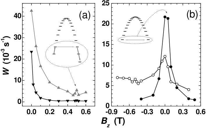
Fig. 4.6 : (a) Longitudinal field dependence of the NSLR rate in ZFC sample at $T=20$ mK (down triangles) and $T=720$ mK (up triangles). The measuring frequency in these datasets is $\nu=231+\gamma_{N}B_{z}$ MHz. (b) Longitudinal field dependence of the NSLR rate in FC (open circles) and ZFC (full circles) sample at $T=20$ mK, with measuring frequency $\nu=230+\gamma_{N}B_{z}$ MHz. The insets are sketches of the electron spin transitions responsible for the observed features.

Fig. 4.6(a) also shows a comparison between $W(B_{z})$ at $T=20$ and 720 mK, thus just at the edge of the thermally activated regime. It appears that both $W(0)$ and the width of the resonance increase by raising the temperature. In addition, at $T=720$ mK an extra small peak appears at $B_{z}\simeq 0.5$ T, which value coincides with the first level crossing for slow-relaxing molecules. Since the peak is not visible at 20 mK, we may attribute it to tunneling of slow molecules through higher excited doublets, e.g. $S_{z}=-9\rightarrow+8$, which becomes favorable as soon as the thermally activated regime is approached (§3.2.3). Moreover, the fact that $W(B_{z})$ at $T=720$ mK and fields $0<B_{z}<0.5$ T is largely increased as compared to the data at 20 mK, would confirm that the thermal activation in FRMs becomes an important source of relaxation already much below 0.8 K, as already argued from the analysis of the slope of $W(T)$ in the quantum regime.

In Fig. 4.6(b) we compare the ZFC data of Fig. 4.5 with a similar field scan of $W(B_{z})$ at $T=20$ mK for an FC sample. We notice that in the FC case it is possible to define both positive and negative longitudinal fields, i.e. corresponding to whether $B_{z}$ is applied parallel or opposite to the magnetization of the sample. One may observe in Fig. 4.6(b) that the shape of the resulting field-dependence is asymmetric, in a way that resembles the asymmetry of the dipolar field distribution (Fig.3.10). On the other hand, the width in the FC is much larger than in the ZFC sample, contrary to the prediction for $B_{\mathrm{dip}}$. Moreover, as mentioned before, the dipolar field distribution is one order of magnitude narrower than the peaks in $W(B_{z})$. At increasingly large negative fields (where negative means opposite to the magnetization the sample) $W(B_{z})$ stabilizes to a rather high plateau with a small anomaly around $B_{z}\simeq-0.5$ T. We shall suggest a possible explanation for the high values of $W(B_{z})$ in FC sample at negative fields when discussing Fig. 4.19 in §4.4.2.

The peak at $B_{z}\simeq 0.5$ T in ZFC sample at 720 mK and the anomaly at $B_{z}\simeq-0.5$ T in FC sample suggest that tunneling in slow-relaxing molecules may also give a contribution under special conditions like high $T$ or inverted magnetization. An important and interesting observation is that, contrary to the TSSR (cf. Fig. 4.4), at zero applied field the NSLR is faster in the ZFC than in the FC sample [111]. Since we argued above that intercluster nuclear spin diffusion should be faster for the FC than for the ZFC sample, this would indicate that there are more tunneling events in a ZFC sample. As mentioned before, such an observation is only possible thanks to the fact that NMR is sensitive to magnetic fluctuations rather than to macroscopic changes in the magnetization.

We also investigated the field dependence of the TSSR rate, but we encountered an unexpected and rather intriguing phenomenon: already for $\left|B_{z}\right|\gtrsim 0.05$ T, the decay of transverse magnetization is characterized by a “chaotic region” that appears after a few milliseconds, as shown in Fig. 4.7. In other words, after an initially well-behaving decay, the echo intensity fluctuates at random, although it always remains below the envelope that can be extrapolated from the first part of the decay. In the same way, by measuring several times the echo intensity with the same delay between pulses, one would randomly find any intensity between zero and the height of the extrapolated envelope. Also, the extension of the initial well-behaving decay tends to reduce with increasing field. Such a chaotic behavior is observed both in FC and ZFC samples, and both in Mn⁴⁺ and Mn³⁺ sites (see §4.2.4). We stress that this has nothing to do with instrumental noise: at any point we see a clean echo signal, just the amplitude and the phase are totally random. We don’t have an explanation for this phenomenon, but it’s intriguing to remark that 0.05 T is just the maximum spread of the dipolar bias distribution (Fig. 3.10).

Fig. 4.7 : Decay of transverse magnetization at $T=20$ mK in ZFC sample, with an applied field $B_{z}=0.2$ T. Notice the chaotic behavior after about 5 ms. The solid line is a fit to Eq. (4.3) in the first part of the decay.

By fitting just the initial part of the decay we can still tentatively extract the field dependence of the TSSR rate $T_{2}^{-1}(B_{z})$. Unfortunately, on such a short interval it is not possible to separate the gaussian and exponential contributions to the decay, thus we fitted all the data to Eq. (4.3) which for the zero-field dataset gives just an average value. Given the circumstances it’s not easy to evaluate the error bars, but we may assume them to be rather large. Fig. 4.8 shows a comparison between $W(B_{z})$ and $T_{2}^{-1}(B_{z})$, both normalized to the zero-field value. As it appears, the field dependencies of the NSLR and TSSR rates are quite similar, although curiously the similarity seems closer for the positive field direction, relative to the FC sample. Moreover, the observation that the TSSR is faster in a FC than in ZFC sample remains valid when $B_{z}\neq 0$.

We suggest that there is a possibility to explain at the same time the resemblance of the field dependencies of NSLR and TSSR rates and the efficiency of the intercluster nuclear spin diffusion. The tunneling in fast-relaxing molecules produces a fluctuating dipolar field, such that the Zeeman energy of ⁵⁵Mn nuclei in equivalent sites of neighboring molecules also fluctuates in time; in this way, there is a chance that at some instant the nuclei in different molecules will have precisely the same Zeeman splitting and will therefore easily undergo a flip-flop transition. If we accept this mechanism as responsible for the efficiency of the intercluster spin diffusion, then it’s clear that by applying a longitudinal field the drastic reduction of tunneling rate should also decrease the probability that two nuclei in neighboring clusters would come at exact resonance, resulting in a reduction of the TSSR rate with the same field dependence as the NSLR rate, as indeed observed.

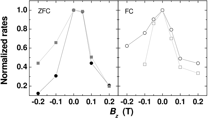
Fig. 4.8 : Comparison between the field dependencies of the NSLR (circles) and TSSR (squares) rates, normalized to the zero-field value, in ZFC (left panel) and FC (right panel) sample, at $T=20$ mK.

4.2.3 Deuterated sample

The role of the fluctuating hyperfine bias on the incoherent tunneling dynamics of SMMs, predicted by Prokof’ev and Stamp (§3.6), has been very clearly demonstrated by measuring the quantum relaxation in Fe₈ crystals where the hyperfine couplings were artificially modified by substituting ⁵⁶Fe by ⁵⁷Fe or ¹H by ²H [16]. For instance, the time necessary to relax 1% of the saturation magnetization below 0.2 K was found to increase from 800 s to 4000 s by substituting protons by deuterium, whereas it decreased to 300 s in the ⁵⁷Fe enriched sample. We already mentioned in §3.6.2 that the “tunneling window” for the cluster spin is most effectively enlarged by those nuclei that easily coflip with the cluster spin. In SMMs, this is indeed the case for the nuclei located at ligand molecules (like ¹H) because their local field is the sum of the dipolar fields from several clusters, whereas the ⁵⁵Mn or the ⁵⁷Fe nuclei are less likely to coflip since the hyperfine fields they experience before and after the flip are almost exactly antiparallel.

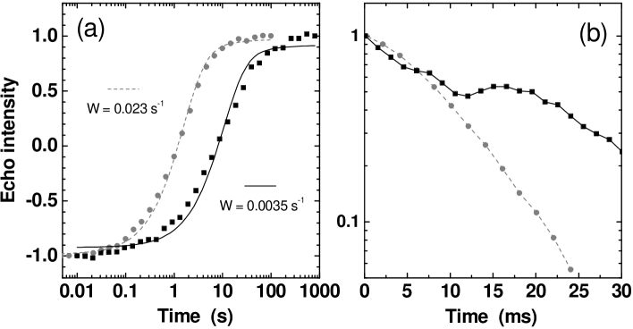
Fig. 4.9 : Comparison between the nuclear inversion recoveries (a) and the decays of transverse magnetization (b) in the ”natural” Mn₁₂-ac (circles) and in the deuterated sample (squares), at $T=20$ mK in zero field and ZFC sample, for the Mn⁽¹⁾ site. The solid lines in (a) are fits to Eq. (4.1).

In this sense, it is understandable that the largest effect on the tunneling rate is seen by isotope substitution of ¹H by ²H. The deuterium nuclei have spin $I=1$ but their gyromagnetic ratio is 6.5 times lower than for protons. This is the reason why, in the framework of the PS theory, one expects indeed a reduction of the incoherent tunneling rate due to the weaker (fluctuating) hyperfine bias. Since in Mn₁₂-ac the only possible isotope substitution is ¹H $\rightarrow^{2}$H, we performed a short set of measurements on a deuterated sample. The sample consists of much smaller crystallites than the “natural” ones used in all other experiments reported in this chapter. Despite having been prepared following the same procedure as described in §4.1, the orientation of the deuterated sample turned out to be almost completely random, probably due to the too small shape anisotropy of the crystallites. We report therefore only experiments in zero external field, where the orientation is in principle irrelevant.

The results are shown in Fig. 4.9: the ⁵⁵Mn NSLR rate at $T=20$ mK in zero field and ZFC sample is indeed reduced to $W_{\mathrm{deut}}\simeq 0.0035$ s^-1, i.e. precisely 6.5 times lower than in the “natural” sample! This clearly points to a reduction of the electron spin tunneling rate of the same type as observed in the deuterated Fe₈ [16], and confirms once more that the NSLR is determined precisely by such tunneling fluctuations. As regards the TSSR, the results is very intriguing: slow but rather ample oscillations are superimposed to the decay of transverse magnetization, somehow reminiscent of what is observed in the natural sample upon application of a small field (Fig. 4.7), but without the chaotic features. Fitting the average decay constant [Eq. (4.3)] yields $T_{2}^{-1}\simeq 38$ s^-1, i.e. a TSSR $\sim 2.5$ times slower than in the natural sample. Such reduction is consistent with the hypothesis that the intercluster nuclear spin diffusion is helped by the fluctuation of the bias on the nuclear Zeeman levels when tunneling events occurs (§4.2.2). As a matter of fact, both the NSLR and the TSSR in the deuterated sample are rather similar to the data in the “natural” sample with an applied field $B_{z}\simeq 0.05$ T. The oscillations in the decay of transverse magnetization remain an obscure phenomenon, but observing them even in this zero-field experiment seems to rule out instrumental artifacts, and suggests that something bizarre happens in the nuclear spin-spin interactions as soon as the tunneling fluctuations slow down below a certain threshold.

4.2.4 Comparison with a Mn³⁺ site

Some rather intersting results come from the analysis of extra measurements performed on the NMR line of the Mn⁽²⁾ site, i.e. a Mn³⁺ ion, which at low temperature is centered at $\nu^{(2)}\simeq 283.7$ MHz. We didn’t follow the whole temperature evolution of the spectrum, but comparing our data with the previous experiments[89, 87] at higher $T$ it seems that the resonance line has slightly shifted to higher frequencies upon cooling.

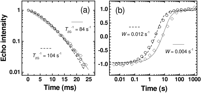
Fig. 4.10 : Comparison between the decay of transverse magnetization (a) and the recovery of longitudinal magnetization (b) in Mn⁽¹⁾ (circles) and Mn⁽²⁾ (diamonds) sites, at $T=20$ mK in FC sample and zero external field. The solid (Mn⁽²⁾) and dashed (Mn⁽¹⁾) lines are fits to Eq.(4.4) in panel (a) and Eq.(4.1) in panel (b).

Fig.4.10 shows a comparison between the decay of transverse magnetization and the recovery of the longitudinal magnetization in Mn⁽¹⁾ and Mn⁽²⁾ sites, at $T=20$ mK in FC sample and zero external field. The TSSR is very similar in both sites, although a closer inspection evidences that the gaussian nature of the decay is less pronounced in the Mn⁽²⁾ sites, which leads to $T_{2G}^{-1}=84$ s^-1 instead of the $T_{2G}^{-1}=104$ s^-1 found in Mn⁽¹⁾. More importantly, the NSLR is three times slower in the Mn⁽²⁾ site, as seen in Fig. 4.10(b). This is opposite to the high-$T$ regime[89, 95], where the Mn³⁺ sites were found to have much faster relaxation. Furthermore, the field dependence of the NSLR rate appears sharper in the Mn⁽²⁾ site, as shown in Fig.4.11. The asymmetry in $W(B_{z})$ for a FC sample is still present, but less evident than in the Mn⁽¹⁾ site due to the more pronounced decrease of $W$ already for small applied fields. These results suggest that the tunneling in fast-relaxing molecules is less effective in relaxing the nuclei in a Mn³⁺ site than in a Mn⁴⁺ site, although the intercluster nuclear spin diffusion appears to work comparably well. In fact, the measured TSSR rate is mainly determined by intercluster spin diffusion between nuclei in slow molecules, since the nuclear spins in FRMs are just a small minority. On the contrary, the NSLR rate is determined by the combination of tunneling in FRMs and nuclear spin diffusion between fast and slow molecules. Since the FRMs differ from the majority clusters precisely in the electron spin arrangement of the Mn³⁺ sites, it is conceivable that this would be an obstacle for the coupling between the nuclei in Mn³⁺ sites of fast and slow molecules, which are no longer equivalent, whereas the Mn⁴⁺ sites remain relatively unaffected by the distortion in FRMs. This would explain both the much slower NSLR because of the “broken link” between nuclei in fast and slow molecules, and the slightly slower TSSR where we just notice the “absence” of the small fraction of nuclei located at the FRMs from the participation to intercluster spin diffusion.

When the temperature is increased such that also the slow-relaxing molecules start to have considerably fast tunneling fluctuations via higher excited levels ($T>0.8$ K), the problem of bad nuclear spin diffusion at Mn³⁺ sites between fast and slow molecules becomes irrelevant. We may then expect that the NSLR in Mn³⁺ sites is produced by the combined action of the fluctuating transverse hyperfine field due to intrawell excitations [the model on which Eq. (3.25) is based], plus the effect of thermally-assisted tunneling. In Mn⁴⁺ sites the first contribution should be absent, which could explain why the NSLR in the thermally-activated regime is lower than in Mn³⁺ sites.

We may therefore conclude that most if not all the different data presented in §4.2 can be consistently explained within our model of tunneling in FRMs plus intercluster nuclear spin diffusion.

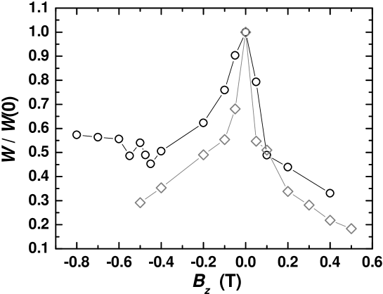
Fig. 4.11 : Longitudinal field dependencies of the NSLR rates in Mn⁽¹⁾ (circles) and Mn⁽²⁾ (diamonds) sites, normalized at the zero-field value. The data are taken at $T=20$ mK in FC sample with central measuring frequencies $\nu^{(1)}(0)=230$ MHz and $\nu^{(2)}(0)=283.7$ MHz.

4.3 Effects of strong perpendicular fields

In this section we describe the effects on the NSLR rate of a strong magnetic field $B_{\perp}$, applied perpendicular to the anisotropy axis. The interpretation of the NSLR is tightly related to the NMR spectra, which provide useful information about the orientation of the crystallites and the crossover between ⁵⁵Mn and ¹H Larmor frequencies.

4.3.1 NMR spectra

In a single crystal having the $\hat{c}$-axis exactly perpendicular to the external field, the three ⁵⁵Mn NMR lines should evolve as in Fig. 3.9, neglecting the possibility of delocalization of the spin wave functions (§3.3.2). Our sample consists of a large number of crystallites, oriented (within a certain spread) along an axis which is orthogonal to both the external field and the axis of the NMR coil. In this way, whatever is the canting angle of the electron spins towards the external field, the total field at the nuclei is always perpendicular to the axis of the NMR coil.

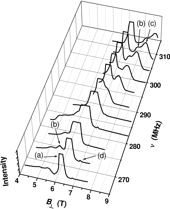
Fig. 4.12 : Field-sweep NMR spectra taken at $T=20$ mK. Several features, marked by letters, are visible and discussed in the text. The high and chopped peak observed in the range $6-7$ T is due to the protons in the sample.

Fig. 4.12 shows field-sweep spectra taken at $T=20$ mK. The sample can be considered as saturated, since we applied 9 T before starting the sweeps. By this procedure we expect most of the cluster spins to be aligned in the same direction within each crystallite, except eventually for those crystallites that are oriented perpendicular to the field within a fraction of a degree. The signal belonging to the protons (a) is recognizable by the chopped top; in fact, the ¹H line is so intense that it saturates the receiver on this scale, and to observe it properly we had to attenuate the input by at least 30 dB. Focusing on the Mn⁽¹⁾ line, we observe that at low frequencies and fields the signal is characterized by a peak (b), plus a more spread-out background that we attribute to misoriented crystallites. The peak fits indeed with the calculated position for crystallites with easy axis oriented at an angle $\theta_{B}=88^{\circ}-90^{\circ}$ with the field (see below), as explained in §3.3.2. By increasing the field, line (b) crosses and is retrieved on the right hand side of line (a), but now two peaks are clearly visible. The peak on the right, labelled (c), tends to increase in intensity at the expenses of (b) when moving to higher fields and frequencies. For instance, the ratio between the amplitudes of the (b) and (c) peaks is 0.73 at $\nu=303.2$ MHz and 0.67 at $\nu=311$ MHz. An extra series of small and sharp peaks (d) is also visible on the right hand side of the ¹H line for $\nu\lesssim 290$ MHz.

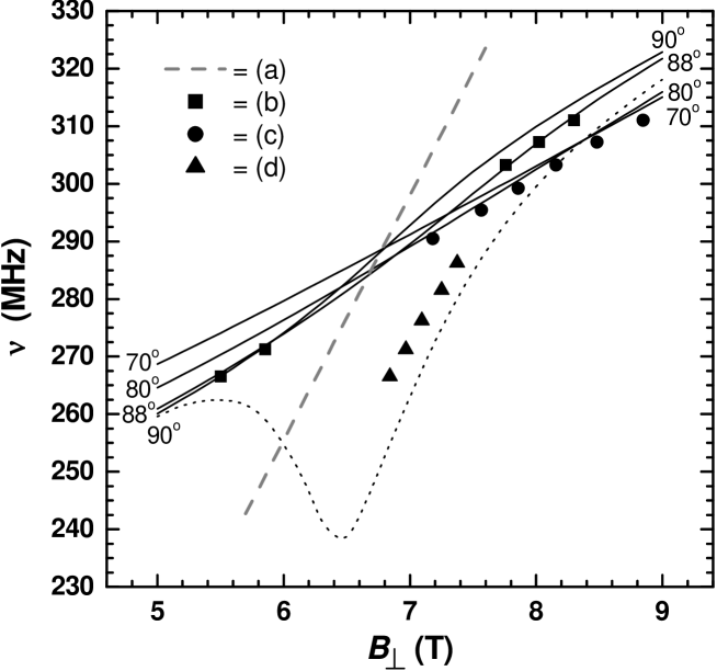
Fig. 4.13 : Positions of the peaks in the field-sweep NMR spectra: the symbols correspond to lines (b), (c) and (d) as specified in the inset. For the protons (a) only the calculated central value is given, plotted as a dashed gray line. Solid lines are calculated spectra according to Eq. (3.18), with the indicated orientation of the $z$ axis relative to the magnetic field. The dotted line is the calculated spectrum for $\theta_{B}=90^{\circ}$, taking into account the reduction of the total spin by quantum superposition [Eq. (3.21)]

In Fig. 4.13 we report the positions of all these peaks and compare them with the calculations. It is then clear that, of the two broad peaks at $B_{\perp}>7$ T and $\nu>295$ MHz, the left must indeed be the continuation of line (b) corresponding to nuclei in crystallites oriented at $88^{\circ}$ from the field. Remarkably, if line (b) at low fields contained contributions from crystallites at $\theta_{B}\simeq 90^{\circ}$ (it’s hard to believe that this would not be the case), they seem to have disappeared at higher fields. The right peak (c), of increasing height, could have two origins. On the one hand, the calculated spectra for $\theta_{B}=70^{\circ}-80^{\circ}$ tend to accumulate precisely around the position of (c), thus the signal intensity that is found in the region 5 T - 270 MHz should in principle pile up just around (c) for $7.5<B_{\perp}<8.5$ T. On the other hand, for $B_{\perp}>8$ T the tunneling splitting becomes so large (Fig. 3.4) as to overcome the bias $\xi$ originating from the longitudinal component of the dipolar fields, but also that arising from the misalignment of the crystallites as long as $(90^{\circ}-\theta_{B})$ is not too large. One may expect (§3.3.2) the NMR signal intensity to start being displaced towards the calculated line for delocalized electron spins, beginning with the best aligned crystallites and involving more and more amounts of sample as $B_{\perp}$ increases. This may explain why, upon increasing $B_{\perp}$, line (c) seems to grow at the expenses of line (b), and why there is no trace of signal at $\theta_{B}\simeq 90^{\circ}$. Most likely, a detailed description of the NMR spectra involves a combination of the phenomena mentioned above.

One may ask to what extent can we trust such fine-detailed comparisons between measured and calculated spectra, in view of the fact that the parameters of the spin Hamiltonian are affected by some uncertainty. We found out that the calculations are in fact very robust, since the effect of varying the spin Hamiltonian parameters, even over a range much wider that the accepted error margins for the commonly used values, is hardly visible on the scale of Fig. 4.13.

The extra small line (d) is rather fascinating: its position is in fact close to the calculated spectrum for a perfectly oriented crystallite, where the total spin falls into a symmetric superposition of $|\Uparrow\rangle$ and $|\Downarrow\rangle$ as soon as $\Delta>\xi_{D}$ (§3.4, Fig 3.11). This calculation, contrary to those performed assuming $S=10$ (solid lines in Fig. 4.13), is extremely sensitive to the values of the parameters of the spin Hamiltonian. One could easily allow the dotted line in Fig. 4.13 to be drawn just on top of the data, by varying the parameters in the calculation within a reasonable margin. To further investigate this issue we measured field-sweep spectra on another sample, consisting of deuterated Mn₁₂-ac crystallites having an almost random orientations (§4.2.3). Line (d) is still visible but its intensity is even smaller than shown in Fig. 4.12. Moreover, it continues linearly down to at least 230 MHz, i.e. much lower than expected from the calculation (cf. Fig. 3.11), without showing any turning point. The most plausible origin of line (d) is therefore a set of ¹H nuclei very close to the magnetic core and experiencing an extra dipolar field $\simeq 0.6$ T; in the deuterated sample, the intensity is further reduced because of the substitution of most of the ¹H by ²H. The ⁵⁵Mn signal in the deuterated sample does not yield well-resolved peaks because of the random orientation of the crystallites.

The NMR lines corresponding to nuclei in Mn³⁺ sites, whose calculated frequencies for $\theta_{B}=90^{\circ}$ are shown in Fig. 3.9, are broader and less intense than the Mn⁽¹⁾ line [89, 87]. The distribution of $\theta_{B}$ broadens their spectrum even further, such that their contribution to the measured signal is basically just a uniform background.

Finally, we remark that all the discussion made so far is relative to ⁵⁵Mn nuclei in Mn⁽¹⁾ sites of standard, slow relaxing molecules. Nuclei in fast-relaxing molecules have their resonance frequency shifting much more quickly to higher values, because the lower anisotropy implies that the electron spin can cant more easily towards the field. Moreover, the direction of the local hyperfine field in FRMs is likely to deviate from the crystallographic $\hat{c}$-axis even n zero applied field (§3.2.4), yielding an extra contribution to the spread of the resonance line.

4.3.2 NSLR in perpendicular fields

In view of the results described in §4.2, it appeared very interesting to check whether the possibility to increase the tunneling splitting by means of a perpendicular field can give visible features in the NSLR rate $W(B_{\perp})$. One would expect an acceleration of the tunneling rate and therefore an increase of $W$; in reality, the problem is made more complicated by the misalignment of the crystallites with respect to the field, and by the fact that, at low fields, the tunneling dynamics is provided only by FRMs. Whatever the orientation of a crystallite may be, it is very unlikely that many FRMs will be exactly perpendicular to the field, since their local anisotropy axis does not coincide with $\hat{c}$. As a consequence, one would expect any external field to effectively destroy the tunneling dynamics of most of the FRMs.

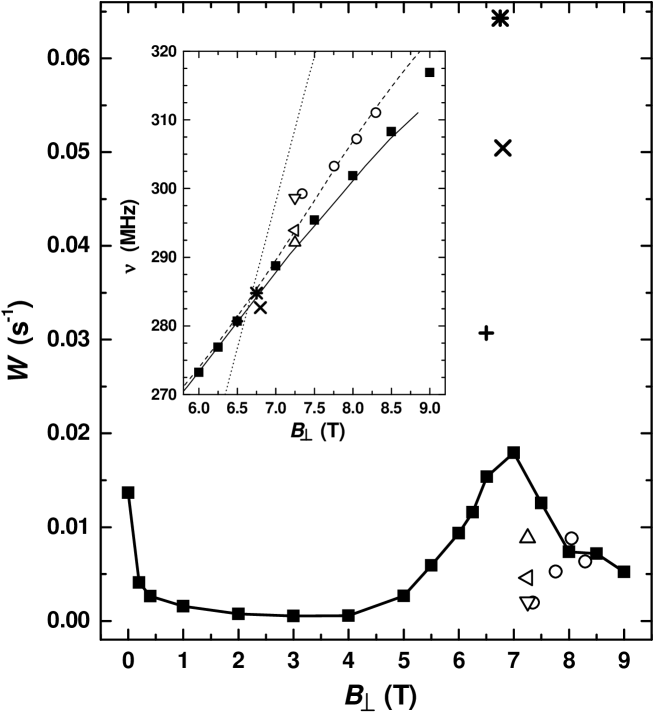
Fig. 4.14 : NSLR rate as function of perpendicular field at $T=20$ mK, following the highest signal intensity (squares), at the crossing between ¹H and ⁵⁵Mn (crosses), at $B_{\perp}>7.25$ T as function of frequency (triangles), and along line (b) (circles). The inset shows the measuring frequency for each set of datapoints (same symbols as in the main panel), compared with line (c) (solid), line (b) (dashed) and line (a) (dotted).

Fig. 4.14 shows $W(B_{\perp})$ at $T=20$ mK; the values of $W$ are obtained by fitting the inversion recoveries to Eq. (4.2), i.e. by a stretched exponential. As expected, as soon as $B_{\perp}>0.2$ T we observe a strong reduction of $W$, due to the suppression of tunneling in FRMs. For $B_{\perp}>4$ T, the NSLR starts to accelerate again: at this point $\Delta\sim 10^{-5}$ K, already larger than in most FRMs, but the effect of misalignment can still be very important. At higher fields it becomes essential to specify at which position we take the data. The main results (square symbols) obey the criterion of maximal signal intensity at a given field: in practice, line (b) for $B_{\perp}<6.5$ T and line (c) for $B_{\perp}>6.5$ T.

At $B_{\perp}\simeq 6.7$ T, the Mn⁽¹⁾ line crosses the protons line, which is 30 dB more intense that the ⁵⁵Mn line because of the much larger number of protons present in each molecule. This fact makes it is very easy to recognize when protons are involved, but it also means that the Mn⁽¹⁾ signal is in fact completely masked by the ¹H signal when the crossing of the Larmor frequencies occurs. The measured NSLR (crosses in Fig. 4.14) must therefore be interpreted as the NSLR of the protons.

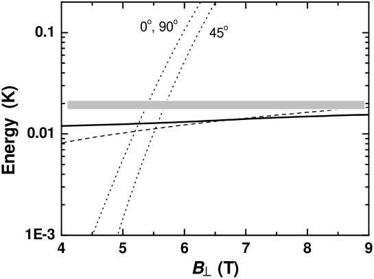
Fig. 4.15 : Perpendicular field dependencies of the Zeeman energies in Mn⁽¹⁾ (solid) and ¹H (dashed), the tunneling splitting (dotted) for the indicated orientations in the $xy$ plane, and the thermal energy (grey shadow).

By increasing $B_{\perp}$ above 7 T, $W(B_{\perp})$ starts to decrease again. As shown in Fig. 4.15, the tunneling splitting is at this point much higher than both the thermal and the nuclear Zeeman energies. Under these conditions, due to depopulation of the upper level of the tunnel-split ground doublet, the electron spin fluctuations should indeed slow down, consistent with the observation of a Schottky anomaly in the field-dependent specific heat $C_{m}(B_{\perp})$ [11, 112] which occurs at the crossing between thermal energy and tunneling splitting. Although the transition rate between the symmetric ground state and the antisymmetric excited state is here measured less directly than in a specific heat experiment, the largely similar field dependencies of $W(B_{\perp})$ and $C_{m}(B_{\perp})$ for 5 T $<B_{\perp}<9$ T points to a common physical origin for the two phenomena. The crossing between Mn⁽¹⁾ and ¹H lines also gives rise to an apparent increase in the NSLR, but this is simply due to the fact that the protons line is itself characterized by a higher NSLR rate, and completely masks the Mn⁽¹⁾ line. On the other hand, as seen in Fig. 4.12, the crossing range should be limited to the $6.5-7$ T range and is therefore definitely not wide enough to justify the whole peak in $W(B_{\perp})$.

We remark that the mentioned possibility to observe the field dependence of the NSLR from time-dependent specific heat experiments has interesting implications. In order to measure the hyperfine contribution to $C_{m}$, the nuclei must be able to absorb heat quickly enough as compared to the experimental time window of the specific heat experiment ($\sim 100$ s). Indeed, this condition was observed to hold only for $B_{\perp}>5$ T [112].

Fig. 4.16 : Perpendicular field dependence of the stretching exponent $\alpha$ for the inversion recovery (4.2), at $T=20$ mK.

Two extra sets of data points have been measured. One set (circles in Fig. 4.14) is taken along line (b) on the high-field side, i.e. where crystallites with $\theta_{B}\simeq 88^{\circ}$ are expected to show up, and shows an apparently opposite behavior compared to line (c), since $W(B_{\perp})$ strongly decreases just where it would go towards a maximum on line (c). The other dataset (triangles) is taken at constant $B_{\perp}=7.25$ T while shifting the frequency towards lower values, i.e. moving from line (b) to line (c). Indeed $W$ grows along that direction. These observations are difficult to understand if we interpret line (c) as the bunching of the signal coming from crystallites oriented at $70^{\circ}-80^{\circ}$ from the field, since with such misalignment in the field range $7-9$ T the two lowest energy levels are separated by at least 10 K, due to the large longitudinal bias. One would then expect the electron spin fluctuations to be totally frozen at $T=20$ mK. As mentioned when discussing Fig. 4.12, it is also possible that line (c) contains (at least for a part of its total intensity) a signal from a growing fraction of molecules that are very well oriented perpendicularly and whose electron spin occupies stably the symmetric ground state. The excitations to the antisymmetric state would then represent tunneling oscillations of the cluster spin, and, given the magnitude of $\Delta$ in this regime, we may even expect such oscillations to be coherent for fairly long times [12]. If we adopt this picture, (c) should be a highly inhomogeneous line, consisting of a mixture of signals from very well oriented ($\theta_{B}=88^{\circ}-90^{\circ}$) and badly misoriented ($\theta_{B}<80^{\circ}$) crystallites. In this case one expects the inhomogeneity of the line to show up in the stretching exponent $\alpha$ of the inversion recovery (§4.1). Fig. 4.16 shows that $\alpha(B_{\perp})$ is indeed a good indicator for the inhomogeneity of the signal: it first decreases smoothly up to $B_{\perp}\sim 6$ T, then shows an abrupt dip where also the protons participate to the signal, finally it keeps decreasing quite steeply along line (c), possibly because of the increasing contribution of nuclei from well aligned molecules in their symmetric ground state.

4.4 Nuclear spin temperature

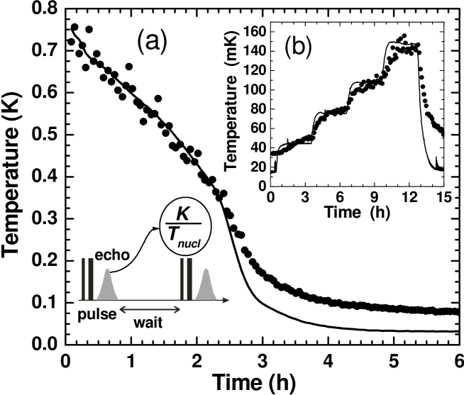
Fig. 4.17 : Comparison between bath temperature $T_{\mathrm{bath}}$(solid lines) and nuclear spin temperature $T_{\mathrm{nucl}}$ (circles), while cooling down the system (a) and while applying step-like heat loads (b). The inset illustrates how $T_{\mathrm{nucl}}$ is obtained from the NMR data. The waiting time between NMR pulses was 60 s in (a) and 180 s in (b). Both datasets are at zero field in ZFC sample.

A crucial issue in the nuclear spin dynamics of single-molecule magnets is to which extent the nuclear spin temperature [113] is able to follow the lattice temperature (as determined by the phonons in the molecular crystal), and what is the mechanism that links the two systems. To our knowledge there is neither experimental nor theoretical work published on this topic so far.

4.4.1 Time-evolution of the nuclear spin temperature

We have investigated this problem by cooling down the refrigerator from 800 mK to 20 mK while monitoring simultaneously the temperature $T_{\mathrm{bath}}$ of the ³He bath in the mixing chamber (just next to the sample) and the NMR signal intensity of the Mn⁽¹⁾ line, checked by an echo pulse sequence every 60 s, in zero external field and on a ZFC sample. The nuclear spin temperature $T_{\mathrm{nucl}}$ is obtained as described in §4.1, and plotted in Fig. 4.17 together with $T_{\mathrm{bath}}$. We find that the nuclear spin temperature indeed strictly follows the bath temperature, with a small deviation below $\sim 200$ mK that we attribute to the heating effects of the NMR pulses. In fact, the pulse rate used in this experiment is ten times higher than in all the measurements shown in §4.2, so it is likely that not all the energy provided to the nuclear spin system can dissipate to the ³He stream at such a rate. We therefore repeated the experiment at the lowest temperatures applying a pulse train every 180 s and step-like heat loads. As shown in the inset of Fig. 4.17, $T_{\mathrm{nucl}}$ indeed follows quite accurately $T_{\mathrm{bath}}$ except for a remaining discrepancy at the lowest $T$, but now much less evident than in the previous experiment with high pulse rate.

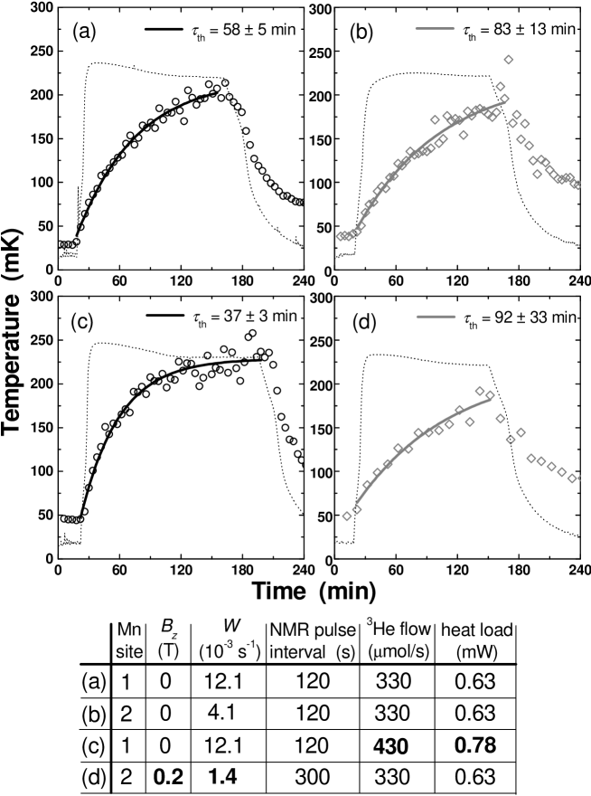
Fig. 4.18 : Time evolution of the nuclear spin temperature (open symbols) and the bath temperature (dotted lines) upon application of a step-like heat load. The solid lines are fits to Eq. (4.7), yielding the thermal time constants $\tau_{\mathrm{th}}$ reported in each panel. All data are for an FC sample, with the Mn site, external magnetic field $B_{z}$, NSLR rate $W$, NMR pulse waiting time, ${}^{3}He$ flow rate and applied heat load as given in the annexed table.

The application of step-like heat loads is a useful method to investigate the effective time constant $\tau_{\mathrm{th}}$ for the thermalization of the nuclear spin system with the helium bath, in particular the relationship between $\tau_{\mathrm{th}}$ and the NSLR rate $W$ as obtained from the inversion recovery technique and discussed in §4.2. This can be done by monitoring $T_{\mathrm{nucl}}$ in different longitudinal fields and different Mn sites, by which we can easily change the NSLR rate. Since also the NMR signal intensity changes under each different condition, we must redefine every time the conversion factor $K$ between signal intensity and $T_{\mathrm{nucl}}$. Moreover the monitoring pulse rate must be adjusted as well, and we found that it is indeed the combination of pulse rate and NSLR rate that determines the discrepancy between the observed lowest spin temperature and the base temperature of the refrigerator. Upon heating up to, say, 200 mK, this effect becomes irrelevant as seen in the inset of Fig. 4.17. It is therefore a natural choice to define $K$ in such a way that the asymptotic value of $T_{\mathrm{nucl}}$ matches the measured $T_{\mathrm{bath}}$ at the end of the heat step. Fig. 4.18 shows four examples of the time evolution of $T_{\mathrm{nucl}}$ under the application of a heat load for $\sim 2$ hours, in Mn⁽¹⁾ and Mn⁽²⁾ sites, with or without an applied field, and with an increased ³He flow rate. We fitted the data to the phenomenological function:

$$T_{\mathrm{nucl}}(t)=T_{\mathrm{nucl}}(0)+[T_{\mathrm{nucl}}(\infty)-T_{\mathrm{nucl}}(0)]\left[1-\exp\left(-\frac{t-t_{0}}{\tau_{\mathrm{th}}}\right)\right],$$ (4.7)

where $T_{\mathrm{nucl}}(\infty)$ is set by definition equal to $T_{\mathrm{bath}}$ at the end of the step, $T_{\mathrm{nucl}}(0)$ follows automatically from the above constraint, and $t_{0}$ is the time when the heat pulse is applied. We find that $\tau_{\mathrm{th}}$ is always much longer than the nuclear relaxation time $T_{1}\sim 1/2W$, and that the dependence on Mn site and applied field is not proportional to the change in $T_{1}$ under different conditions. What really seems to make the difference is the ³He flow rate: within the errors, the ratio of heat transfer from the ³He stream to the nuclear spins is proportional to the ³He flow rate, given the same conditions of nuclear site and external field. This confirms that the thermal contact between nuclear spins and lattice phonons is quite fast, as we demonstrated by the values of the NSLR rate, and that the main bottleneck is at the interface between the crystallites, the embedding epoxy and the ³He stream.

4.4.2 Effect of large magnetic fields and superradiance

To conclude this section we discuss an issue which may be relevant to most of the experiments on quantum tunneling studied by magnetization loops or fast field-sweeps. While sweeping the magnetic field in such a way that many cluster spins are forced to flip, also the hyperfine fields at the nuclear sites are being inverted at an abnormal rate. One may then ask whether the nuclear spin system remains in thermal equilibrium, or the macroscopic inversion of the electron spin polarization leads to a remarkable increase of $T_{\mathrm{nucl}}$. To answer this question we performed a full magnetization loop $0\rightarrow-8.5\rightarrow+8.5\rightarrow 0$ T at a sweep rate $|\mathrm{d}B_{z}/\mathrm{d}t|=0.5$ T/min on a sample with initial positive magnetization and measured $T_{\mathrm{nucl}}$ as soon as the loop was finished, with the field back to zero. Because of the continuous shift of the resonance frequency it would have obviously been impossible to monitor $T_{\mathrm{nucl}}$ during the field sweep. As shown in Fig. 4.19, we find that $T_{\mathrm{nucl}}$ at the end of the field sweep is much higher than $T_{\mathrm{bath}}$. Interestingly, the evolution of $T_{\mathrm{nucl}}$ is characterized by an initially very fast decay, whereas after a few minutes $T_{\mathrm{nucl}}$ relaxes to its equilibrium value with precisely the same time constant $\tau_{\mathrm{th}}\simeq 57$ min as already found in the heat transient experiment in Fig. 4.18(a). By extracting $T_{\mathrm{nucl}}(\infty)$ from the fit to Eq. (4.7) and imposing that it should be the same also for the initial fast decay, we refitted just the very first datapoints obtaining $T_{\mathrm{nucl}}(0)\sim 350$ mK and $\tau_{\mathrm{th}}^{\mathrm{(initial)}}\simeq 300$ s. The latter value is still a bit longer than $T_{1}=(2W)^{-1}\simeq 40$ s in FC sample at $T=20$ mK [see Fig. 4.10(b), open circles] but not incompatible with the idea that the very first part of the relaxation is the real spin-lattice relaxation, whereas afterwards the equilibrated lattice and spins relax to the bath temperature at the usual rate mainly determined by the ³He circulation.

Fig. 4.19 : Time evolution of $T_{\mathrm{nucl}}$ (open symbols) measured with NMR pulse intervals of 180 s on the Mn⁽¹⁾ line just after a magnetic hysteresis loop performed with a field sweep rate $|dB_{z}/dt|=0.5$ T/min. The sample is FC with initial positive magnetization. The dashed and solid lines are fits to Eq. (4.7) for the fast (initial) and slow part of the relaxation, respectively, having imposed $T_{\mathrm{nucl}}(\infty)=49$ mK for both fits. The inset shows $B_{z}$ and $T_{\mathrm{bath}}$ during the field sweep: notice that the time scale in the main panel is the continuation of the one in the inset.

In the inset of Fig. 4.19 we also report $B_{z}$ and $T_{\mathrm{bath}}$ as a function of time during the field sweep. $T_{\mathrm{bath}}$ remains rather stable around 35 mK except at two special points, $-1.9$ T sweeping down and $+1.9$ T sweeping up, where it suddenly jumps to $\sim 100$ mK. We notice that this occurs only when $B_{z}$ is opposite to the instantaneous magnetization, and that in fact $|B_{z}|=1.9$ T is a level crossing field for the electron spins in slow-relaxing molecules, which suggest that the phenomenon may be due to magnetic avalanches. A similar heat emission was already observed by specific heat experiments [114], but at $T\sim 2-3$ K. On the other hand, it is rather surprising to find that the main heat emission takes place already at $B_{z}=\pm 1.9$ T, i.e. the fourth level crossing, whereas it is known[106] that small Mn₁₂-ac crystals at very low $T$ start to appreciably invert their magnetization only at $B_{z}\sim\pm 4$ T. Moreover we know from experience that, because of the large volume of our refrigerator, it is virtually impossible to heat the ³He bath so abruptly as it appears in the inset of Fig. 4.19. In fact, such a sudden temperature increase resembles very much the effect we find when applying a NMR pulse (cf. Fig. 2.5): we first observe a sharp peak in the measured $T$, which is due to the direct heating of the thermometer by the rf-pulse, and only in the subsequent minutes we observe a smooth temperature increase, when the thermometer indeed senses the heating of the ³He bath. In a recent work [115], Tejada et al. report the observation of radiation emitted by a large amount of Mn₁₂-ac crystals when measuring magnetic hysteresis loops. In their experiment the radiation bursts are observed at $B_{z}=\pm 1.4$ T, thus the third level crossing, but the measurements are performed at $T=1.8$ K, much higher than in our case. The proposed explanation is based on the phenomenon of superradiance [116]: when the wavelength of the radiation emitted by each electron spin flip is greater than the size of the sample, large numbers of spins may tunnel simultaneously because they interact with a common radiation field, thereby producing radiation avalanches. A prerequisite for this phenomenon to occur is indeed a population inversion, in this case a total electron spin magnetization opposite to the direction of the applied field, which is precisely what we observe.

In fact, even though the thermometer detects only the radiation bursts produced by large avalanches, we may expect that weak hints of superradiance could occur even at small values of $B_{z}$, provided that the magnetization is opposite to the field. An example is given by the data in Fig. 4.6(b), where we investigated the NSLR rate in a FC sample with “positive” magnetization, and observed indeed that $W(B_{z})$ shows a surprisingly high plateau for $B_{z}<0$. An argument against the attribution of that plateau to weak hints of superradiance could be that we didn’t notice any substantial changes in the sample magnetization while performing those measurements. On the other hand, we are still speaking about relatively low values of $W$, which would not require an extremely high number of tunneling events. A pragmatic solution to this puzzle would be given only by continuously repeating the same nuclear relaxation experiment (e.g. at $B_{z}=-0.5$ T) and checking whether $W$ changes in time, in the same way as the total magnetization.

4.5 Proposal for a unifying theory

We are now at a stage to gather all the experimental results discussed so far and use them as basic elements to build a complete description of the quantum dynamics of the coupled system “cluster spins + nuclei”. The starting framework is the Prokof’ev-Stamp theory (§3.6), but we shall supplement it with some extra assumptions in order to account for the observed intercluster nuclear spin diffusion and the thermal equilibrium between nuclear spins and lattice phonons.

4.5.1 Basic assumptions

The model we are going to set up is based upon the following (experimentally justified) starting points:

(i) the tunneling dynamics takes place only in fast-relaxing molecules, whereas the neighboring slow molecules can be safely considered as frozen during the timescale of interest. For our purpose, the slow molecules serve simply as a “reservoir of nuclear polarization”;

(ii) for the ease of discussion, we assume that every cluster is coupled to $N$ nuclear spins $I=1/2$, and that the hyperfine field $\vec{B}_{\mathrm{hyp}}$ always lies along the $\vec{z}$ axis; upon tunneling, the direction of $\vec{B}_{\mathrm{hyp}}$ is turned by $180^{\circ}$. The latter assumption simulates indeed the real situation for ⁵⁵Mn nuclei in Mn₁₂-ac. We also define a local nuclear polarization for the $i$-th cluster $\Delta N(i)=N_{i}^{\uparrow}-N_{i}^{\downarrow}$ along the $+\vec{z}$ axis, and the associated local hyperfine bias $\xi_{N}(i)=\hbar\gamma_{N}\Delta N(i)\vec{B}_{\mathrm{hyp}}\cdot\vec{z}$. Notice that the sign of $\xi_{N}(i)$ depends on the instantaneous direction of $\vec{B}_{\mathrm{hyp}}$, whereas the sign of $\Delta N(i)$ does not.

(iii) nuclei in neighboring clusters are coupled by dipole-dipole interactions that lead to intercluster nuclear spin diffusion. Experimentally, the spin diffusion rate is quite fast: we may therefore assume that any sudden change in local hyperfine bias is quickly redistributed among all clusters in order to attain the equilibrium within the nuclear spin system.

For all other aspects we rely on the Prokof’ev-Stamp model for the description of the coupling between central spin and nuclei. We assume therefore that the hyperfine interactions split the electron spin levels into a manifold of states, indexed by $\Delta N$ and broadened by intracluster nuclear spin diffusion, spanning a total width $\Xi_{N}=\xi_{N}^{(\mathrm{max})}-\xi_{N}^{(\mathrm{min})}=N\hbar\gamma_{N}B_{\mathrm{hyp}}$. From assumption (ii) it follows that, since $\vec{B}_{\mathrm{hyp}}$ only takes two antiparallel directions ($\Rightarrow\omega_{k}^{\perp}=0$), the hyperfine-split manifolds on either sides of the anisotropy barrier are simply the mirror of each other. In the absence of external bias, to any state with $\Delta N^{(1)}$ on the left side of the barrier corresponds a state with $-\Delta N^{(2)}$ on the right side. Also, $\omega_{k}^{\perp}=0$ implies that the tunneling of the central spin does not produce any coflipping of nuclear spins by the “orthogonality blocking” mechanism (§3.6.1), i.e. $\kappa\simeq 0$. Furthermore, the “topological decoherence” is negligible as well; the typical nuclear Larmor frequencies are $\omega_{N}\sim 10^{9}$ s^-1, whereas the tunneling traversal time (§3.2.3) is $\tau_{\mathrm{tr}}\sim\Omega_{0}^{-1}\sim 10^{-12}$ s. In the PS language, this leads to $\lambda\sim N(\omega_{N}/\Omega_{0})^{2}\simeq 0$. All this means that the only allowed tunneling transitions are those that do not require any coflip of nuclear spins, i.e. $\Delta N=const.$; the relevant tunneling splitting is therefore $\Delta_{0}$. On basis of the assumption (iii) about the internal equilibrium in the nuclear spin system we may write the nuclear spin temperature $T_{\mathrm{nucl}}$ in terms of the populations of nuclear Zeeman levels. For this purpose it is convenient to introduce the populations of the nuclear Zeeman levels relative to the local direction of $B_{\mathrm{hyp}}$, $N_{+}$ and $N_{-}$, where $N_{+}$ is the number of nuclei per cluster that are in the Zeeman ground state, and $N_{-}$ counts the nuclei in the excited state:

$$\frac{\langle N_{-}\rangle}{\langle N_{+}\rangle}=\exp\left(-\frac{\hbar\omega_{N}}{k_{B}T_{\mathrm{nucl}}}\right),$$ (4.8)

where $\langle\ \rangle$ indicates the average over all the clusters in the sample. Calling $n=N_{+}-N_{-}$, $\langle N_{+}\rangle=(N+\langle n\rangle)/2$, $\langle N_{-}\rangle=(N-\langle n\rangle)/2$ and $\langle\xi_{N}\rangle=-\hbar\omega_{N}\langle n\rangle$, (4.8) becomes:

$$\frac{\Xi_{N}+\langle\xi_{N}\rangle}{\Xi_{N}-\langle\xi_{N}\rangle}=\exp\left(-\frac{\hbar\omega_{N}}{k_{B}T_{\mathrm{nucl}}}\right).$$ (4.9)

4.5.2 Tunneling mechanism

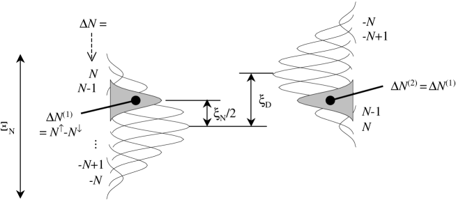
Fig. 4.20 : Sketch of a possible configuration where tunneling may occur in the presence of a dipolar bias $\xi_{D}$. The gray areas represent the nuclear polarization groups on opposite side of the barrier having the same $\Delta N$, such that tunneling does not require any nuclear coflips. In order to populate one of those groups, an initial hyperfine bias $\xi_{N}=\xi_{D}$ must be achieved via intercluster nuclear spin diffusion.

In the absence of an external bias on the cluster electron spin, tunneling would take place only when $\xi_{N}=0$ as well, since the polarization groups with $\Delta N=0$ are the only ones having equal energy and equal nuclear polarization. In the more general case where we include the quasi-static dipolar bias $\xi_{D}$ arising from neighboring clusters, the tunneling transition with $\Delta N=const.$ can still take place, but requires now an initial hyperfine bias $\xi_{N}=\xi_{D}$. After the tunneling, since $\vec{B}_{\mathrm{hyp}}$ is now reversed, the hyperfine bias becomes $-\xi_{D}$; in other words, the effect of tunneling is in fact to convert the hyperfine energy into dipolar energy or vice versa. A sketch of the situation is depicted in Fig. 4.20: starting from a cluster where the electron spin is favorably aligned with respect to the dipolar field produced by the neighbors, a tunneling transition requires “charging” the local nuclei up to polarization group where $\xi_{N}=\xi_{D}$, such that on the opposite side of the barrier there is another polarization group having identical $\Delta N$. After tunneling, the cluster spin is oriented opposite to the local dipolar field, and the required energy has been taken from the nuclear reservoir, which is now in a favorable polarization state with respect to the new direction $\vec{B}_{\mathrm{hyp}}$.

It is clear that intercluster nuclear spin diffusion is an essential ingredient to attain the condition $\xi_{N}=\xi_{D}$ at all. Flip-flop processes between nuclei in different clusters conserve the total energy of the nuclear system, but allow the local hyperfine bias to wander through the whole hyperfine-split manifold until the tunneling resonance is found. A tunneling event like in Fig. 4.20 would have the effect of “locally extracting” an energy $\xi_{D}$ from the nuclear spin system; by the same mechanism of intercluster spin diffusion, this energy can then be redistributed among the neighbors, thereby attaining an effective reduction of the nuclear spin temperature. On the other hand, the tunneling process can work in the opposite direction, reducing the dipolar energy at the expenses of an increase of $T_{\mathrm{nucl}}$.

Let us recall that this picture, in particular as a consequence of assumption (ii), accounts only for nuclei like ⁵⁵Mn in Mn₁₂-ac, i.e. nuclei where the hyperfine fields flips by $180^{\circ}$ when a tunneling event occurs. We have shown in §4.2.3 that actually the most important role in triggering the incoherent tunneling dynamics is played by nuclei such as protons, precisely because they have a large coflipping probability due to the non-antiparallel directions of $\vec{B}_{\mathrm{hyp}}^{(1)}$ and $\vec{B}_{\mathrm{hyp}}^{(2)}$. In that case, the condition $\Delta N=const.$ may be relaxed to $|\Delta N^{(1)}-\Delta N^{(2)}|\leq 2M$, where $M$ is the number of coflipping nuclei. Although such an extension is essential to properly account for the tunneling rate of the electron spin, we shall not include it in our discussion as long as we focus on the tunneling-driven nuclear relaxation of ⁵⁵Mn (which is the main subject of our experiments) rather than the hyperfine-driven tunneling rate of the electron spin.

4.5.3 Coupling with lattice phonons

So far we have not introduced any thermostat to set the temperature to which the equilibrium $T_{\mathrm{nucl}}$ should relax. The only natural way to obtain a certain equilibrium nuclear spin temperature from the tunneling mechanism described above, is to assume detailed balance between the rate $w^{\downarrow}$ of the transitions that reduce $T_{\mathrm{nucl}}$ at the expenses of dipolar energy (like in Fig. 4.20), and the rate $w^{\uparrow}$ for transitions in the opposite direction:

$$\frac{w^{\uparrow}}{w^{\downarrow}}=e^{-\xi_{N}/k_{B}T}.$$ (4.10)

On the other hand, as long as the tunneling rates are derived from the standard Prokof’ev-Stamp expression (3.44), there’s no way to distinguish between $w^{\downarrow}$ and $w^{\uparrow}$.

We propose therefore that, in order to account for the observed equilibrium between nuclear spin and lattice temperatures, the PS theory must be extended to include the possibility of inelastic tunneling events, accompanied by creation or annihilation of lattice phonons. In particular, we argue that an essential role could be played by the time-dependence of the dipolar bias $\xi_{D}$ that arises when the distance between neighboring clusters is modulated by a phonon. Due to the peculiar structure of single-molecule magnets, containing very rigid clusters bound by soft organic ligands, we may expect a clear separation between the intracluster, high-energy phonon modes, and the intercluster low-energy modes, corresponding to the relative displacement of the clusters considered as rigid objects. This approach has been already successfully used to account for the Mössbauer recoil-free fraction in metal cluster molecules [117], which are bound by similarly soft ligands, yielding a Debye temperature $\Theta_{D}\sim 10-20$ K for intercluster phonon modes. In some sense, this idea is a “molecular version” of the well-known Waller mechanism [118] for the spin-lattice relaxation of paramagnetic ions. The problem is that, if used to estimate the nuclear spin-lattice relaxation rate in the standard way, i.e. by calculating the spectral density of the fluctuating dipolar field directly at the nuclear sites [119], the Waller mechanism would lead to extremely long relaxation times. What we suggest is that the Waller mechanism can be regarded as a source of fluctuating bias producing a similar effect as the nuclear spin diffusion in the PS theory (§3.6.1); similar conclusions on the effect of the Waller mechanism could be drawn by using the Landau-Zener formalism (see §3.2.3 and §3.6.3) to calculate the probability of incoherent tunneling while the dipolar bias sweeps through the tunneling resonance. We already remarked in §3.6.3 that the tunneling rate $\tau_{T}^{-1}$ obtained in this way is independent of the bias sweep rate, in this case the frequency of the phonon modulating $\xi_{D}$. $\tau_{T}^{-1}$ does depend on the range of fluctuation $\hbar\Gamma_{\mu}$, whose role would here be taken by the amplitude $\Delta\xi_{D}$ of the change in dipolar bias arising from lattice strain associated with the phonon modes. By inspecting Eq. (3.44) one finds that the prefactor $\propto\Delta^{2}/\Gamma_{\mu}\rightarrow\Delta^{2}/\Delta\xi_{D}$ in $\tau_{T}^{-1}$ is inversely proportional to the amplitude of fluctuation. On the other hand, the extra factor $e^{-|\xi|/\xi_{0}}$ may lead to at least a partial cancellation effect if $\Delta\xi_{D}$ contributes to $\xi_{0}$ as well, which could justify the approximately $T$-independent NSLR rate found below 0.8 K. Since the fluctuation of dipolar bias has to be combined with the fluctuating hyperfine bias, deriving the exact expression for the inelastic tunneling rate constitutes a very challenging but formidable theoretical task, that largely exceeds the scope of this thesis.

4.5.4 Nuclear spin-lattice relaxation rate

Irrespective of the precise expressions for $w^{\uparrow}$ and $w^{\downarrow}$, their deviation from the average value $\tau_{T}^{-1}=(w^{\uparrow}+w^{\downarrow})/2$ will be very small, unless the temperature becomes much lower than the typical range of the dipolar interaction $\xi_{D}\sim 0.1$ K. The reason why the relevant energy scale is $\xi_{D}$ and not $\hbar\omega_{N}$ is that, in our model, the nuclear spin system can change its global polarization only by converting hyperfine energy into dipolar energy ($\xi_{N}=\xi_{D}$). In the extreme case where $\xi_{D}=0$ in all clusters, all tunneling events would take place at $\Delta N=0$, with no effects on the nuclear spins. In fact, it would be very intriguing to find a system where $\hbar\omega_{N}\gg\xi_{D}$ (e.g. by diluting the magnetic clusters) and check if the thermalization of the nuclear spins works as efficiently as we find here.

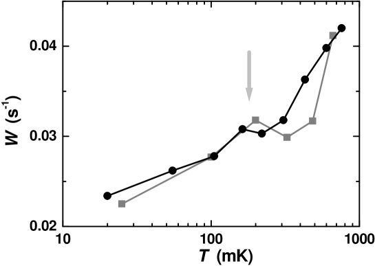
Fig. 4.21 : NSLR rate in the quantum regime, for Mn⁽¹⁾ site in ZFC sample and zero external field. Circles are the same data as in Fig. 4.3, squares are from an experiment carried out in a different run several months before: the arrow indicates the position of the weak maximum in $W(T)$ around 180 mK.

Furthermore, by focusing on the NSLR rate $W(T)$ only in the quantum regime, we have noticed that the “roughly” $T$-independent plateau has not only a slope, but also a slight and broad maximum around $T\simeq 0.18$ K, below which $W(T)$ tends to decrease somewhat more steeply. As shown in Fig. 4.21, by measuring $W(T)$ in the quantum regime in two independent runs, we got the impression that the maximum around 0.18 K is a weak albeit reproducible feature. The value of 0.18 K may not be a coincidence in view of the fact that, as we discuss in chapter V, a system like Mn₆ orders ferromagnetically at $T_{c}=0.16$ K purely by the effect of dipolar interactions. It would be very interesting to see whether a fully developed theoretical description can account for this peak in $W(T)$, and if this is indeed related to the dipolar interaction energy.

An estimate of the NSLR rate in the quantum regime can be obtained by writing a master equation for the populations of the nuclear Zeeman levels relative to the local hyperfine field direction, $N_{+}$ and $N_{-}$ (cf. §4.5.1). For simplicity, since the internal equilibrium is reestablished within a time $T_{2}\ll\tau_{T}$ after each tunneling event, we assume that just before tunneling all clusters have the same values of $N_{+}$ and $N_{-}$, neglecting fluctuations around the mean values. If a fast-relaxing molecule tunnels at time $t$, the polarization of its own nuclei is abruptly inverted. Each time a tunneling transition lowers the energy of the local nuclei, which occurs at a rate $w_{\downarrow}$, then $N_{-}$ nuclei have been added to the total number of nuclei in the Zeeman ground state. After a time $T_{2}$ this decrease in local hyperfine bias has been redistributed over the sample: calling $x$ the fraction of FRMs over the total, then the tunneling event has increased $N_{+}$ to $N_{+}+xN_{-}$. The same reasoning holds for transitions that increase the hyperfine bias. The master equation is therefore:

$$\frac{\mathrm{d}N_{+}}{\mathrm{d}t}=xN_{-}w_{\downarrow}-xN_{+}w_{\uparrow}.$$ (4.11)

From here the NSLR rate can be obtained by standard textbook calculations [120]. Writing $N_{+}=(N+n)/2$ and $N_{-}=(N-n)/2$, (4.11) becomes:

$$\frac{\mathrm{d}n}{\mathrm{d}t}=xN(w_{\downarrow}-w_{\uparrow})-xn(w_{\downarrow}+w_{\uparrow}),$$ (4.12)

which can be rewritten as:

$$\frac{\mathrm{d}n}{\mathrm{d}t}=2W(n_{0}-n),$$ (4.13)

$$n_{0}=N\frac{w_{\downarrow}-w_{\uparrow}}{w_{\downarrow}+w_{\uparrow}},$$ (4.14)

$$W=x\frac{w_{\downarrow}+w_{\uparrow}}{2}=x\tau_{T}^{-1},$$ (4.15)

where $n_{0}$ is the equilibrium nuclear polarization and $W$ is the desired NSLR rate, since the solution of (4.13) is precisely of the form $n(t)=n(0)-[n(0)-n_{0}][1-\exp(-2Wt)]$.

Comparing Eq. (4.15) with the experimental value of $W\simeq 0.03$ s^-1 reported in §4.2.1, one would deduce that, for instance, 1% of FRMs tunneling at a rate $\tau_{T}^{-1}\sim 3$ s^-1 is sufficient to explain the data. Such a tunneling rate is high but not unreasonably high, especially considering the FRMs having two flipped Jahn-Teller axes and a barrier $\sim 15$ K (§3.2.4). We recall that for an easy-axis spin $S\gg 1$, described by a Hamiltonian $\mathcal{H}=-DS_{z}^{2}+ES_{x}^{2}$ with $D\gg E$, the tunneling rate is proportional to $D(E/D)^{S}$ [58]. By simply reducing the height of the barrier by a factor 4, we may already expect an increase of five orders of magnitude in the tunneling rate with respect to a normal molecule! FRMs are also likely to have higher values of $E$, thereby increasing the tunneling rate even further.

Let us remark that the interplay between electron spin (tunneling) fluctuations and nuclear spin diffusion is completely different from the standard picture of relaxation by paramagnetic impurities [121]. In the presence of an impurity spin, the closest nuclei are relaxing very fast because of the strong fluctuations, but the static component of the field produced by the impurity drives them out of resonance with respect to the nuclei that are farther away: one finds that nuclear spin diffusion starts to work only outside a sphere whose radius is determined by the strength of the nuclear dipolar coupling compared with the field produced by the impurity. In this sense, intercluster nuclear spin diffusion in SMMs is a very peculiar phenomenon, since all the nuclei are equivalent and there is no minimum radius for the spin diffusion.

4.6 Conclusions

We now briefly summarize the results presented in this chapter, in order to place them in a complete framework of observations and interpretations, and in particular to make clear what the breakthroughs of our research are.

(i) Incoherent quantum tunneling of the electron spin provides a relaxation channel for the nuclear spin system, and its effects are much more pronounced than expected [14]. This can be deduced from the roughly $T$-independent plateau in the ⁵⁵Mn NSLR rate below 0.8 K, and from the coincidence between maxima in the NSLR rate and tunneling resonances for the electron spins. The observation of the effect of tunneling on the nuclear spins can be done even in zero field and demagnetized sample, thus without any changes in the macroscopic magnetization of the cluster spins. We also suggest that the correct interpretation of the observed NSLR for $T>0.8$ K should include the effect of thermally-assisted tunneling as well.

(ii) The intercluster nuclear spin diffusion is fast on the timescale of the NSLR and of the electron spin tunneling rate. Its existence can be inferred from the $T$-independent value of the TSSR rate below 0.8 K, and from the $\simeq\sqrt{2}$ ratio between the TSSR rates in a fully polarized and a demagnetized sample. This is the first direct experimental observation of such a phenomenon in SMMs. Moreover, the field dependencies of NSLR and TSSR suggest that the fluctuating dipolar field produced by tunneling events may play a role in facilitating the intercluster nuclear spin diffusion.

(iii) The tunneling dynamics in zero external field is ascribed to the fast-relaxing molecules present in any real sample of Mn₁₂-ac. This follows from both a quantitative analysis of the NSLR rate, and from the experimental observation that the macroscopic magnetization of the sample does not change during the measurements. Furthermore, the comparison between NSLR and TSSR in Mn⁴⁺ and Mn³⁺ sites indicates that the intercluster nuclear spin diffusion between FRMs and normal molecules is less efficient between nuclei in Mn³⁺ sites, which are precisely those where the FRMs are different.

(iv) The isotope substitution of ¹H by ²H leads, as expected, to a significant decrease of the incoherent tunneling rate, which manifests itself in a congruent reduction of the NSLR and TSSR rates.

(v) The application of strong perpendicular fields produces a broad peak in the NSLR rate which is consistent with the observed increase of excitations within the tunneling-split ground doublet, as previously observed by field-dependent specific heat experiments [11].

(vi) Even in the regime ($T<0.8$ K) where the nuclear spins are relaxed only by ground state quantum tunneling of the electron spins, the nuclear spin temperature remains in equilibrium with the bath temperature. This is a new and unexpect result, and its implication have never been included in any theoretical discussion. We attempt to account for this observation by a suggesting a model that combines the Prokof’ev-Stamp theory with the effect of modulation of the intercluster dipolar fields (Waller mechanism), in order to elucidate how the cluster spin tunneling can relax the nuclear spins, and why it is necessary to attribute different rates to tunneling transitions that increase rather than decrease the nuclear spin energy.

(vii) Experiments where a longitudinal magnetic field is applied opposite to the direction of the sample magnetization could be interpreted by assuming the presence of magnetization avalanches, which also manifest themselves in the form of electromagnetic radiation [115].

Chapter 5 Long-range dipolar ordering in Mn₆

Few examples of long-range magnetic order induced by purely dipolar interactions are known as yet [122, 123]. Therefore, the possibility to study such phase transitions and the associated long-time relaxation phenomena in detail in high-spin molecular cluster compounds, with varying crystalline packing symmetries and different types of anisotropy, presents an attractive subject [124, 125]. However, for the most extensively studied molecular clusters sofar such as Mn₁₂, Fe₈ and Mn₄ [126, 127, 109, 112] the uniaxial anisotropy experienced by the cluster spins is very strong. Consequently, the electronic spin-lattice relaxation time $T_{1}^{el}$ becomes very long at low temperatures and the cluster spins become frozen at temperatures of the order of 1 K, i.e. much higher than the ordering temperatures $T_{c}\sim 0.1$ K expected on basis of the intercluster dipolar couplings [124, 125, 128]. Although quantum tunneling of these cluster spins has been observed [126, 127, 109, 112], and could in principle provide a relaxation path towards the magnetically ordered equilibrium state [124, 125], the associated rates in zero field are extremely small ($<100$ s^-1). For these systems, tunneling only becomes effective when strong transverse fields $B_{\perp}$ are applied to increase the tunneling rate. Although the tunability of this rate and thus of $T_{1}^{el}$ by $B_{\perp}$ could recently be demonstrated for Mn₁₂, Fe₈ and Mn₄ [112], no ordering has yet been observed.

The obvious way to obtain a dipolar molecular magnet is thus to look for a high-spin molecule having sufficiently weak magnetic anisotropy and negligible inter-cluster super-exchange interactions. Here we report data for
Mn₆O₄Br₄(Et₂dbm)₆, abbreviated as Mn₆ [85], whose net magnetocrystalline anisotropy (cf. §3.2.5) proves to be sufficiently small to enable measurements of its equilibrium magnetic susceptibility and specific heat down to our lowest temperatures ($15$ mK).

In this chapter we report the observation that the magnetic clusters do undergo a transition to a long-range ferromagnetically ordered state at $T_{c}=0.161(2)$ K. The transition can be observed both by ac-susceptibility and by specific heat experiments, thanks to the fact that the magnetic relaxation remains very fast, even at very low temperatures, as compared to the intrinsic experimental times ($0.1-5$ ms for ac-susceptibility and $1-100$ s for specific heat). The magnetic relaxation has been investigated by field-dependent specific heat and ⁵⁵Mn NMR. By combining the two techniques we are able to study the interplay between electron- and nuclear- spin-lattice relaxation.

5.1 Long-range ferromagnetic ordering

5.1.1 ac-susceptibility

The ac-susceptibility data in Fig. 5.1 were taken using the susceptometer described in §2.3, varying the frequency $\nu$ between $230$ to $7700$ Hz and recording the data while slowly cooling down the refrigerator. Additional measurements at $T>1.8$ K were performed in a commercial SQUID susceptometer. For this zero-field experiment, the susceptometer was mounted in the upper Araldite pot of the dilution refrigerator (cf. Fig. 2.1), after having replaced the Kapton tail by a closed plug. This has the advantage of allowing a higher ³He circulation rate, and assuring a the perfect coincidence of the sample and thermometer temperatures even for $T>0.8$ K, when some rather sudden temperature jumps may occur.

The real part $\chi^{\prime}$ shows a sharp maximum at $T_{c}=0.161(2)$ K. We found that $\chi^{\prime}$ at $T_{c}$ is close to the estimated limit for a ferromagnetic powder sample, $1/(\rho N_{s}+\rho_{\mathrm{sam}}N_{c})\simeq 0.14\pm 0.02$ emu/g, where $\rho=1.45$ g/cm³ and $\rho_{\mathrm{sam}}\simeq 0.45$ g/cm³ are respectively the densities of bulk Mn₆ and of the powder sample, $N_{s}=4\pi/3$ is the demagnetizing factor of a crystallite, approximated by a sphere, and $N_{c}\simeq 2.51$ is the demagnetizing factor of the sample holder. This indicates that Mn₆ is ferromagnetically ordered below $T_{c}$.

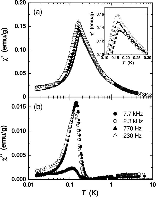
Fig. 5.1 : Real (a) and imaginary (b) parts of the ac-susceptibility at the indicated frequencies. Inset: magnification of $\chi^{\prime}(T)$ to evidence the frequency dependence of the peak.

The temperature $T_{\mathrm{peak}}$ at which the maximum value of $\chi^{\prime}$ is found, as shown in detail in the inset of Fig. 5.1, is seen to vary only weakly with $\nu$, which we attribute to the anisotropy. The total activation energy of Mn₆ amounts to $DS^{2}\simeq 1.5$ K, i.e. about $45$ times smaller than for Mn₁₂. Accordingly, one expects the superparamagnetic blocking of the Mn₆ spins to occur when $T\simeq T_{B}($Mn${}_{12})/45$, that is below $\simeq 0.12$ K. Since this value is close to the actual $T_{c}$, one may expect that for $T\rightarrow T_{c}$ the approach to equilibrium begins to be hindered by the anisotropy of the individual molecular spins. We stress however, that the frequency dependence of $\chi^{\prime}$ observed here is quite different from that of the well known anisotropic superparamagnetic clusters. A way to quantify the frequency dependence of the peak in $\chi^{\prime}$ is by means of the parameter $\Delta T_{\mathrm{peak}}/[T_{\mathrm{peak}}\Delta(\log\nu)]$, which gives the variation of $T_{\mathrm{peak}}$ per decade of frequency. We find here $\Delta T_{\mathrm{peak}}/[T_{\mathrm{peak}}\Delta(\log\nu)]\simeq 0.04$, to be compared with the typical values of $\sim 0.20$ for superparamagnetic blocking. In fact it is closer to the value $\sim 0.06$ found for certain types of spin glasses [129], but the peak found here is much higher and sharper.

Fig. 5.2 : $T$-dependence of the inverse of the real part of the ac-susceptibility. Circles: low-$T$ susceptometer, $\nu=7700$ Hz. Squares: SQUID susceptometer. The inset shows a magnification of the temperature range around $T_{c}$.

Below $T_{c}$, $\chi^{\prime}$ decreases rapidly, as expected for an anisotropic ferromagnet in which the domain-wall motions become progressively pinned. The associated domain-wall losses should then lead to a frequency dependent maximum around $T_{c}$ in the imaginary part, $\chi^{\prime\prime}$, as seen experimentally indeed [cf. Fig. 5.1(b)]. In fact, although the Mn₆ spins can be considered as nearly isotropic at high temperatures, the anisotropy energy is still large compared with the dipolar interaction energy $\mu^{2}/r^{3}\simeq 0.1$ K between nearest neighbor molecules. Thus the ordering should be that of an Ising dipolar ferromagnet.

Susceptibility data $\chi_{i}$ corrected for the demagnetizing field ($\chi_{i}=\chi^{\prime}/[1-(\rho N_{s}+\rho_{\mathrm{sam}}N_{c})\chi^{\prime}]$) follow the Curie-Weiss law $\chi=C/(T-\theta)$ down to approximately $0.3$ K, with $C=0.034(1)$ cm³K/g and $\theta=0.20(3)$ K. The constant $C$ equals, within the experimental errors, the theoretical value for randomly oriented crystals with Ising-like anisotropy $N_{A}g^{2}\mu_{B}^{2}S(S+1)/3k_{B}P_{m}=0.0332$ cm³K/g, where $S=12$, $g=2$, and the molecular weight $P_{m}=2347.06$. The positive $\theta$ confirms the ferromagnetic nature of the ordered phase. From the mean-field equation $\theta=2zJ_{eff}S(S+1)/3k_{B}$, we estimate the effective inter-cluster magnetic interaction $J_{eff}\simeq 1.6\times 10^{-4}$ K, and the associated effective field $H_{eff}=2zJ_{eff}S/g\mu_{B}=3.5\times 10^{2}$ Oe coming from the $z=12$ nearest neighbors.

5.1.2 Specific heat

Additional evidence for the ferromagnetic transition at $T_{c}$ is provided by the electronic specific heat $c_{e}$, shown in Fig. 5.3 [34]. The specific heat of a few milligrams of sample, mixed with Apiezon grease, was measured at low-T in a home-made calorimeter [34, 112] that makes use of the thermal relaxation method. An important advantage of this method is that the characteristic time $\tau_{e}$ of the experiment (typically, $\tau_{e}\simeq 1-100$ seconds at low-T) can be varied by changing the dimensions (and therefore the thermal resistance) of the Au wire that acts as a thermal link between the calorimeter and the mixing chamber of the dilution refrigerator.

The electronic specific heat was obtained by subtracting from the total specific heat the contribution of the lattice, which follows the well-known Debye approximation for low temperatures $c_{\mathrm{lattice}}\propto(T/\Theta_{D})^{3}$, where $\Theta_{D}\simeq 48$ K, as well as the contribution $c_{\mathrm{nucl}}$ arising from the nuclear spins, as discussed in §5.2.1 below. $c_{e}(T)$ reveals a sharp peak at $0.15(2)$ K, indeed very close to the peak in the real part of the ac-susceptibility. Numerical integration of $c_{e}/T$ between $0.08$ K and $4$ K gives a total entropy change of about $3.4k_{B}$ per molecule, which is indeed very close to the value $k_{B}\ln(2S+1)=3.22k_{B}$ for a fully-split $S=12$ spin multiplet. We may therefore attribute the peak to the long-range order of the molecular spins. We note, however, that at $T_{c}$ the entropy amounts to about $1k_{B}$ per spin, showing that only the lowest energy spin states take part in the magnetic ordering.

Fig. 5.3 : $T$-dependence of the electronic specific heat at zero applied field (circles). The dotted line is the Schottky anomaly calculated with $D=0.013$ K. The full line is the Monte Carlo (MC) calculation for an orthorhombic lattice of $1024$ Ising spins with periodic boundary conditions. For each point, $2\times 10^{4}$ MC steps per spin were performed.

5.1.3 Monte-Carlo Simulations

In order to simulate the zero-field specific heat data, Monte-Carlo (MC) calculations were performed by J. F. Fernández (univ. of Zaragoza, Spain) for an $S=12$ Ising model of magnetic dipoles on an orthorhombic lattice with axes $a_{x}=15.7$ Å, $a_{y}=23.33$ Å, and $a_{z}=16.7$ Å, which approximates the crystal structure of Mn₆. The Hamiltonian includes dipolar interaction term as well as the anisotropy term $-DS_{z}^{2}$ given in Eq. (3.15). When dipolar interactions are neglected, the zero field splittings of the $S=12$ multiplet produced by this crystal field term lead to the Schottky anomaly in $c_{e}$ shown by the dotted curve in Fig. 3. The fit in the range above 0.5 K yields $D/k_{B}\simeq 0.013$ K, in good agreement with our above estimates. For $T<0.5$ K the intermolecular dipolar interactions come into play and remove the remaining degeneracy of the lowest-lying $|\pm m\rangle$ spin doublets. The MC simulations show that the ground state is ferromagnetically ordered, as observed, and predict a shape for $c_{e}$ that is in very good agreement with the experiment. In Fig. 5.3, we show $c_{e}$ calculated assuming all molecular easy ($z$) axes to point along $a_{z}$, i.e. one of the two nearly equivalent short axes of the actual lattice. Similar results were obtained for other orientations chosen for the anisotropy ($z$) axis. We note that the Ising simulations give $T_{c}=0.22$ K, which is slightly higher than the experimental $T_{c}=0.161(2)$ K. This difference may be due to the Ising approximation taken for the intercluster dipolar interaction.

Fig. 5.4 : Calculated critical temperature $T_{c}$ as a function of the anisotropy parameter $D$, for classical Heisenberg spins.

In order to pursue this point further, additional MC simulations were performed for the same crystal lattice, but with classical Heisenberg spins replacing the ($S=12$) Ising spins. To investigate the sensitivity to the type of anisotropy, the sign and magnitude of $D$ were varied. These calculations resulted in the phase diagram shown in Fig. 5.4, which we include here since it illustrates the complicated way in which the nature of the actual ground state and the value of $T_{c}$ may depend on the combination of the long-range dipolar interaction and the anisotropy parameter. Although the ground state for this lattice is always ferromagnetic, it can be either “uniaxial”, with strong preference for the $a_{y}$ axis, or “planar”, in the sense that the $a_{x}-a_{z}$ plane becomes an easy plane with a weak preference for a given direction in the plane, as indicated in the figure. Interestingly, the switching point between these orientations is not at $D=0$ but at $D=3$ mK. The reason for this is as follows. Because the crystal lattice under consideration is far from being cubic, the dipolar interaction energy is rather anisotropic. The energy is minimized when the magnetization $\vec{M}$ points in the direction (in the $a_{x}-a_{z}$ plane) shown in the inset, on the left-hand side of Fig. 5.4. Therefore, $\vec{M}$ points along this direction for $D<0$. On the other hand, the energy minimization for $D>0$ is a competing process. Clearly, dipolar interaction must become dominant for sufficiently small values of $D$. The numerical results show that this occurs if $0<D\lesssim 3$ mK. The numerical datapoints in Fig. 5.4 also show that $T_{c}$ varies sharply within the $-0.01<D<0.01$ K range. Because of the discreteness of the MC simulations we can not tell whether $T_{c}$ vanishes at $D\simeq 3$ mK. The lowest numerical value obtained is as small $T_{c}\simeq 0.03$ K at $D\simeq 3$ mK. Outside this narrow range of $D$, $T_{c}$ is already almost equal to the limiting values of $\simeq 0.7$ K and $\simeq 0.3$ K, reached for infinite negative and positive $D$, respectively. Such a variation of $T_{c}$ with anisotropy, as well as the form of the calculated and observed specific heat ordering anomaly, appear to be specific for dipolar interactions. They differ widely from the corresponding behavior known for 3-dimensional (Heisenberg, Ising, XY) ferromagnetic lattices with nearest-neighbor interaction only. For instance, in those models the variation of $T_{c}$ with anisotropy is restricted to about 20% and the $T_{c}$ value is highest for the Ising case.

5.2 Spin-lattice relaxation

The electron- and nuclear- spin-lattice relaxation in Mn₆ is an interesting topic to investigate and compare with the typical behavior of the highly anisotropic SMMs like Mn₁₂-ac. As we shall see, provided that a Zeeman splitting for the electron spin is created by the application of an external field, the nuclear spin dynamics in Mn₆ closely resembles the behavior of the nuclei in Mn₁₂-ac in the thermally activated regime, where the electron spin energy levels are split by crystal-field effects instead.

5.2.1 Field-dependent specific heat

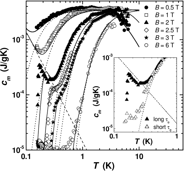
Fig. 5.5 : $T$-dependence of the magnetic specific heat at the specified temperatures. The lines are the calculated electronic (dotted) and nuclear (dashed) contributions. The solid lines are the total (electronic + nuclear) $c_{m}$, calculated accounting for the nuclear $T_{1}$ (see text). Inset: detail of $c_{m}(T)$ at $B=2$ T, for long ($\sim 100$ s) and short ($\sim 1$ s) experimental times.

We begin by discussing the specific heat data obtained in varying magnetic field $B$ [34], plotted in Fig. 5.5. Even for the lowest $B$ value, the ordering anomaly is fully suppressed, as expected for a ferromagnet [130]. Accordingly, we may account for these data with the Hamiltonian (3.15) neglecting dipolar interactions. The Zeeman term splits the otherwise degenerate $|\pm m\rangle$ doublets, and already for $B\sim 0.5$ T the level splittings become predominantly determined by $B$, so that the anisotropy term can also be neglected. As seen in Fig. 5.5, the calculations performed with $D=0$ reproduce the data quite satisfactorily at higher temperatures (dotted curves).

However, when the maxima of the Schottky anomalies are shifted to higher $T$ by increasing $B$, an additional contribution at low $T$ is revealed. It is most clearly visible in the curves for $1$ T$<B<2.5$ T, and varies with temperature as $cT^{2}/R=4\times 10^{-3}$. We attribute this to the high-temperature tail of the specific heat contribution $c_{\mathrm{nucl}}$ arising from the Mn nuclear spins ($I=5/2$), whose energy levels are split by the hyperfine interaction with the Mn³⁺ electronic spins $s$. This interaction can be approximated by $\mathcal{H}_{hf}=A\vec{I}\cdot\vec{s}$, where $A$ is the hyperfine coupling constant (cf. §3.3). At high temperatures (i.e., when $A\,s\ll k_{B}T$) $c_{\mathrm{nucl}}/R\simeq\frac{1}{3}A^{2}s^{2}I(I+1)T^{-2}$ [119]. Taking $A=7.6$ mK as used previously to simulate ESR spectra measured on a Mn₄ cluster [131], we obtain the dashed line shown in 5.5. This contribution was subtracted from the zero-field data shown in Fig. 5.3.

A remarkable feature of the experimental data that is not reproduced by these calculations is that, at the lowest $T$, the nuclear specific heat drops abruptly to about $10^{-5}$ J/gK. The temperature $T_{n}$ where the drop occurs depends on $B$ but also on the characteristic time constant $\tau_{e}$ of our (time-dependent) specific heat experiment: the deviation from the (calculated) equilibrium specific heat is found at a lower $T$ when the system is given more time to relax, as shown in the inset of Fig. 5.5. We conclude that the drop indicates that the ⁵⁵Mn nuclear spins can no longer reach thermal equilibrium within time $\tau_{e}$. We may write:

$$c_{nucl}(\tau_{e})=c_{nucl}^{(\mathrm{eq})}[1-\exp(-\tau_{e}/T_{1})],$$ (5.1)

showing that the transition should occur when the nuclear spin-lattice relaxation time $T_{1}$ becomes of the order of $\tau_{e}$. These transitions to non-equilibrium provide therefore direct information on the temperature and field dependence of $T_{1}$.

As already discussed in §3.5.1, $T_{1}(T,B)$ can be related to the fluctuation of the transverse hyperfine field, as produced by the phonon-induced transitions (at a rate $\tau_{\mathrm{s-ph}}$) between different levels of the electronic spin. In the case of Mn₆ these are simply the Zeeman levels of the $S=12$ cluster spin in the magnetic field $B$, split by an energy $\Delta E=g\mu_{B}B$.

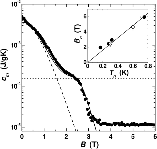
Fig. 5.6 : Field-dependence of the magnetic specific heat at $T=0.3$ K. The dotted line is the calculated electronic specific heat, the dashed line is the equilibrium nuclear specific heat, and the solid line is the calculated total $c_{m}$, accounting for the nuclear $T_{1}$. Inset: $B_{n}(T_{n})$ obtained from $T$-sweeps, as in Fig. 5.5 (full circles), or from $B$-sweeps, as in the present figure (open circles). From the linear fit (solid line) we extract the average $\tau_{0}\simeq 3\times 10^{-4}$ s.

At low $T$ and high $B$, only the ground and the first excited states, $m=+12$ and $m=+11$, need to be considered. We may therefore rewrite Eq. (3.25) as:

$$\frac{1}{T_{1}}=\frac{\gamma_{N}^{2}}{2}\langle\Delta b_{\perp}^{2}\rangle\frac{\tau_{s-ph}}{1+\omega_{N}^{2}\tau_{s-ph}^{2}}\approx\tau_{0}^{-1}\exp\left(-\frac{g\mu_{B}B}{k_{B}T}\right),$$ (5.2)

where $\tau_{0}^{-1}=\langle\Delta b_{\perp}^{2}\rangle/(2B_{\mathrm{tot}}^{2}\tau_{11})$ incorporates the lifetime

$$\tau_{11}=\frac{1-\exp(-g\mu_{B}B/k_{B}T)}{C_{\mathrm{s-ph}}(g\mu_{B}B)^{3}}$$ (5.3)

of the first excited state $m=+11$, and the ratio between the average value of the transverse component of the fluctuating hyperfine field $\Delta b_{\perp}$ and the square of the total field at the nuclei $B_{\mathrm{tot}}$. The approximated expression of (5.2) is valid when $\omega_{N}\tau_{s-ph}\gg 1$, which is practically always the case, except at very low field.

It is easy to see from Eq. (5.2) that the nuclear spins can be taken out of of equilibrium either by decreasing $T$ down to $T_{n}$ at constant field, as in Fig. 5.5), or by increasing $B$ up to a given value $B_{n}$ at constant $T$. This is indeed observed experimentally, as shown in Fig. 5.6. The effect of the field is just to polarize the electron spins, which reduces the fluctuations of the hyperfine field, thus effectively disconnecting nuclear spins from the lattice. It also follows that, for a given $\tau_{e}$, $B_{n}$ is linear in $T_{n}$ as long as the field-dependence of $\tau_{11}$ can be neglected as compared to the exponential dependence of $T_{1}^{-1}$ on $T$ and $B$. The inset of Fig. 5.6 shows $B_{n}(T_{n})$ obtained either from $T$-sweeps at constant $B$ (as in Fig. 5.5) or from $B$-sweeps at constant $T$ (as in Fig. 5.6). The two methods prove to be indeed perfectly consistent with each other. The slope of the linear fit of $B_{n}(T_{n})$ gives an average value of $\tau_{0}\simeq 3\times 10^{-4}$ s in the high-field regime. We observe that at lower fields $B_{n}(T_{n})$ tends to deviate from the linear fit, which we attribute to the decrease of $\tau_{11}$. Using the average value of $\tau_{0}$ we have calculated the time-dependent $c_{\mathrm{nucl}}$ from Eq. (5.1), which has been added to the calculated electronic specific heat to yield the solid lines in Figs. 5.5 and 5.6, and seen to be in good agreement with the experimental data.

5.2.2 ⁵⁵Mn NMR

Fig. 5.7 : Inversion recovery (a) and decay of transverse magnetization (b) for the ⁵⁵Mn nuclei at $T=0.9$ K, $B=5$ T and $\nu=251.5$ MHz. The lines in (a) are fits to Eq. (4.1) (solid), and Eq. (4.2) with $\alpha\simeq 0.5$ (dashed). The solid line in (b) is a fit to Eq. (4.3).

We have now the possibility to compare the NSLR rate as inferred from the specific heat experiments, with direct measurements of this quantity by NMR experiments. The ⁵⁵Mn NSLR and TSSR rates were obtained following the same procedures and analysis as described in §4.1 (Fig. 5.7), but using a standard ³He system instead of the dilution refrigerator. The advantage of the ³He cryostat is that, because of its construction, we do not need to insert a $\lambda$-cable in the NMR resonant circuit (cf. §2.2.2). This increases the quality factor of the resonator and allows to measure large enough signals without need to reach millikelvin temperatures, where the very slow NSLR would make the measurements almost unfeasible. Unfortunately, the useful frequency range becomes accordingly much narrower.

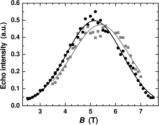
Fig. 5.8 : ⁵⁵Mn NMR spectra at $T=0.9$ K and measuring frequencies $\nu=256.5$ MHz (black circles) and $\nu=261.5$ MHz (gray squares). The gap in the data around $B\simeq 5.8$ T is due to the presence of the ¹H line. The lines are Gaussian fits with total width $2\sigma_{B}\simeq 2.2$ T.

The inversion recoveries [Fig. 5.7(a)] are best fitted by a stretched exponential [Eq. (4.2)] with $\alpha\sim 0.5$, although the choice of the stretching exponent does not strongly influence the extracted value of $W$. The field-sweep NMR spectra in Fig. 5.8 clearly show that it is impossible to determine whether there are inequivalent sites in the molecule, as regards the hyperfine coupling (compare with the case of Mn₁₂-ac in Fig. 3.7). This may be due to the large quadrupolar splitting expected in Mn³⁺ sites, plus the fact that our sample is an unoriented powder. As expected from the internal ferromagnetic structure of the cluster electron spins (cf. §3.2.5), the ⁵⁵Mn spectrum shifts to higher fields by lowering the frequency. The spectra can be fitted by a Gaussian shape with total width $2\sigma_{B}\simeq 2.2$ T; if this width were due to quadrupolar splitting only, it would imply $\Delta\nu_{Q}\sim 7$ MHz, even larger than the highest $\Delta\nu_{Q}\simeq 4.3$ MHz in the Mn⁽²⁾ sites of the less symmetric Mn₁₂-ac cluster. We expect therefore that the random orientation of the crystallites and, eventually, the presence of inequivalent Mn sites as regards the hyperfine coupling, should contribute as well to the observed broadening. Indeed, when decreasing the frequency by 5 MHz the maximum of the spectrum shifts only by 0.24 T, instead of the 0.47 T that would be expected when all the local hyperfine fields are antiparallel to $\vec{B}$. We conclude that the observed spectrum, as well as the NSLR and TSSR data, should be considered as obtained from a mixture of nuclear signals arising from randomly oriented crystallites with largely overlapping and quadrupolar-split NMR lines from all the Mn sites in the cluster. Extrapolating to $B=0$ the field-dependence of the peak of the spectrum, one would obtain $\nu(0)\simeq 360$ MHz $\Rightarrow B_{\mathrm{hyp}}\simeq 34$ T, very similar to the value found in the Mn⁽³⁾ site of Mn₁₂-ac.

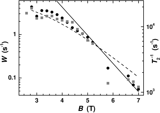
Fig. 5.9 : Field dependencies of the ⁵⁵Mn NSLR (black circles, left scale) and TSSR (grey squares, right scale) at $T=0.9$ K and $\nu=251.5$ MHz. The vertical scales are adjusted to evidence the similar field dependencies. Solid line: calculated $W(B)$ according to Eq. (5.2) with $\tau_{0}=3\times 10^{-4}$ s. Dashed line: fit to Eq. (5.4).

Fig. 5.9 shows the field-dependencies of the NSLR rate $W$ and the TSSR rate $T_{2}^{-1}$, measured at constant frequency $\nu=251.5$ MHz and temperature $T=0.9$ K. From the discussion above it is clear that these data must be interpreted with a certain caution, since shifting $B$ at constant $\nu$ means that we are sampling each time a different portion of the NMR signal, which means different quadrupolar satellites, different orientation of the crystallites, etc. Nevertheless, the agreement with the estimate of $T_{1}$ obtained by specific heat data (inset of Fig. 5.5) is quite satisfactory. We can directly compare the NSLR rate $W(B)$ as obtained by NMR with the estimated $T_{1}$ from specific heat data by plotting the line $W(B)=1/(2T_{1}(B))$ with $T_{1}(B)$ calculated from Eq. 5.2, fixing $\tau_{0}=3\times 10^{-4}$ s and $T=0.9$ K (solid line in Fig. 5.9). The agreement is very good on the high-field side of the data, whereas at low fields the NSLR rate is seen to level off instead of increasing exponentially. This is actually the same phenomenon that we already observed in the low-field part of $B_{n}(T_{n})$ in the inset of Fig. 5.5, due to the fact that $\tau_{0}$ is not constant. We fitted therefore $W(B)$ including the field-dependence of $\tau_{0}$:

$$W(B)\approx\frac{\langle\Delta b_{\perp}^{2}\rangle}{4B_{\mathrm{tot}}^{2}}\times\frac{C_{\mathrm{s-ph}}(g\mu_{B}B)^{3}}{1-\exp(-g\mu_{B}B/k_{B}T)}\exp\left(-\frac{g\mu_{B}B}{k_{B}T}\right).$$ (5.4)

As shown by the dashed line in Fig 5.9, this function indeed fits much better the low-field part of the data.

In Fig. 5.9 we also show the TSSR rate $T_{2}^{-1}(B)$, rescaled in order to evidence the practically identical $B$-dependence as found for the NSLR rate. This is indeed to be expected (cf. §3.5.1 and §3.5.2) if the TSSR is induced by the random change of local hyperfine field when the electron spin makes thermally-assisted transitions between the ground- and the first excited states. Eq. (3.28) can be immediately readapted for Mn₆ by substituting the energy gap $\Delta E=g\mu_{B}B$ and the lifetime of the ground state $\tau_{12}=C_{\mathrm{s-ph}}\Delta E^{3}/[(\Delta E/k_{B}T)-1]$, which yields:

$$T_{2}^{-1}\approx\tau_{12}^{-1}=\frac{C_{\mathrm{s-ph}}(g\mu_{B}B)^{3}}{\exp(g\mu_{B}B/k_{B}T)-1}\approx C_{\mathrm{s-ph}}(g\mu_{B}B)^{3}\exp\left(-\frac{g\mu_{B}B}{k_{B}T}\right),$$ (5.5)

i.e. the same dependence as $W(B)$.

The similarity between NSLR and TSSR rates produced by thermal fluctuations of the electron spin was already observed in the $T$-dependence of $W$ and $T_{2}^{-1}$ in Mn₁₂-ac for $T>0.8$ K (cf. §4.2.1). It is interesting to observe that in Mn₆ we find $T_{2}^{-1}/T_{1}^{-1}\simeq 3800$, i.e. larger than the value $T_{2}^{-1}/T_{1}^{-1}\simeq 1000$ found for the Mn⁴⁺ site of Mn₁₂-ac and much larger that $T_{2}^{-1}/T_{1}^{-1}\sim 200$ for its Mn³⁺ sites [95]. This in fact confirms the hypothesis that a complete description of the NSLR in the thermally-assisted regime of Mn₁₂-ac should include the effect of thermally-assisted tunneling, yielding a contribution to the NSLR which is obviously absent in Mn₆.

5.3 Conclusions

In conclusion, our experiments on Mn₆ demonstrate that dipole-dipole interactions between molecular magnetic clusters may indeed induce long-range magnetic order at low temperatures, provided that the anisotropy is sufficiently small. The spin-lattice relaxation then becomes fast enough to produce equilibrium conditions down to the low temperatures needed. We should add that similar conditions could in principle also be reached in the highly anisotropic cluster systems, for which it was shown that by applying magnetic fields perpendicular to the anisotropy axis, the spin lattice relaxation can be tuned and made similarly fast through the process of magnetic quantum tunneling. However, magnetic ordering phenomena have not been seen in those systems so far. This is most probably due to the fact that, given the magnitude of the fields needed to have a considerable increase of the relaxation rate ($B_{\perp}\gg 1$ T), any longitudinal component of the field would create a Zeeman splitting that is much larger than the energy involved in the magnetic dipolar ordering. We found indeed that in Mn₆ the ordering transition is removed already for relatively small fields ($\sim 0.5$ T).

We have also studied the nuclear spin dynamics of Mn₆, either directly by NMR experiments, or through the hyperfine contribution to the field-dependent specific heat. The agreement between the two techniques is very good, and provides an interesting comparison with the nuclear spin dynamics in the anisotropic SMM Mn₁₂-ac. We find that the splitting of the electron spin levels in Mn₆, as produced by the application of an external field, yields similar features in the nuclear spin dynamics as the crystal field splitting in Mn₁₂-ac. On the other hand, since the quantum tunneling fluctuations are strictly absent in Mn₆, the quantitative comparison of the data confirms that, even in the thermally activated regime, a correct description of the ⁵⁵Mn NSLR of Mn₁₂-ac should include the effects of thermally-assisted tunneling.

Samenvatting

van het proefschrift met de titel:

“Kwantum spin dynamica in Enkel-Molecuul Magneten”

Terwijl de fundamentele wetenschap steeds meer bezig is met onderzoek aan complexe systemen, blijft de industrie investeren in de voortdurende miniaturisering van, bijvoorbeeld, elektronische circuits en geheugens. Deze twee ontwikkelingsrichtingen gaan elkaar ontmoeten op de nanometer-schaal, met gevolg dat de nanowetenschap een zeer belangrijke onderzoeksgebied eordt voor zowel de fundamentele als de toegepaste fysica.

Een van de meest belangwekkende verschijnselen die op de nanometer-schaal kunnen worden bestudeerd is de overgang tussen de klassieke- en de kwantum- fysica. Natuurkundigen zijn gewend aan de toepassing van de kwantummechanica op het atomaire niveau, maar zodra het te beschrijven systeem groter wordt, kunnen sommige aspecten van de kwantummechanica (met name het meet-postulaat) tot paradoxale conclusies leiden (de “Schrödinger kat” paradox). In dit opzicht is de theorie nog niet afgerond, het is dus essentieel om systemen te vinden die geschikt zijn om experimenteel te testen welke factoren van belang zijn voor de overgang tussen kwantum en klassiek gedrag.

Dit proefschrift beschrijft een onderzoek aan het kwantummechanisch gedrag van Enkel-Molecuul Magneten (EMMen). Dit zijn chemische verbindingen die bestaan uit een centrale cluster van magentische ionen, omringd door organische liganden. De magnetische wisselwerking tussen de elektronspins van de ionen in eenzelfde cluster resulteert in een “gigantisch” magnetisch moment (gigantisch t.o.v. de typische waarden voor atomaire momenten) voor de cluster als geheel. De moleculaire magnetische clusters zijn geordend in een kristalstructuur, waarin de moleculaire magnetische momenten (spins) slechts een zwakke onderlinge wisselwerking vertonen, zodat het systeem beschouwd mag worden als een ensemble van identieke nagenoeg onafhakelijke moleculaire spins. Hiermee wordt het mogelijk om de bekende experimentele technieken voor vaste stof fysica toe te passen op de studie van het gedrag van de EMMen. Hoofdstuk II beschrijft de eigenschappen en het ontwerp van de experimentele opstellingen die voor onze onderzoek zijn gebruikt.

Hoofdstuk III is besteed aan de theoretische beschrijving van de fysische eigenschappen van de EMMen. Een essentieel aspect is de magnetische anisotropie, d.v.z. de voorkeur van de cluster spin om zich te orienteren in een van de twee tegenovergestelde richtingen langs een bepaalde voorkeursas. Om de spin om te klappen moet er een bepaalde energie worden toegevoerd, bijvoorbeeld via thermische excitatie. Als het systeem tot een temperatuur veel lager dan de anisotropie energie wordt afgekoeld, dan zijn de cluster spins “bevroren”, wat suggereert dat het mogelijk zou zijn om EMMen te gebruiken als magnetische geheugens, op voorwaarde dat er geen andere mechanisme is dat de richting van de spins kan inverteren.

Dat extra mechanisme bestaat feitelijk wel, als een compleet kwantummechanisch model van de cluster spin wordt toegepast. Omdat twee tegenovergestelde richtingen van de spin dezelfde energie hebben, is er een mogelijkheid voor de spin om te tunnelen door de barrière, d.v.z. zonder dat extra energie wordt toegevoegd. Dit fenomeen bestaat niet in de klassieke fysica, en het is vrij wonderlijk om het te kunnen waarnemen in een zo groot systeem als een EMM. De Prokof’ev-Stamp theorie van het “spin-bad” is een antwoord op de vraag hoe kwantumtunneling in een EMM kan plaatsvinden ondanks zijn koppeling met de omgeving, die normaal gesproken de mogelijkheid voor tunnelen geheel uitsluit. De totale elektronspin van een EMM is magnetisch gekoppeld aan de kernspins in zijn omgeving, maar deze koppeling is sterk beïnvloed door de dynamica van de kernspins. Bovendien, zijn de dipolaire koppeling tussen clusterspins en de invloed van roostertrillingen (fononen) ook van belang voor een nauwkeurige beschrijving van het kwamtumgedrag van EMMen.

Een van de meest aantrekkelijke eigenschappen van de EMMen voor de studie van kwantummechanische verschijnselelen op moleculaire schaal, is dat het mogelijk is om de tunnelwaarschijnlijkheid te veranderen door een extern magnetisch veld aan te leggen, loodrecht op de anisotropie as. Deze “instelbaarheid” is niet alleen handig voor het fundamentele onderzoek, maar geeft ook de hoop om coherente kwantummechanische oscillaties van de cluster spin te kunnen produceren, waardoor de EMMen als basis element voor een kwantumcomputer zouden kunnen worden gebruikt.

We hebben de bovengenoemden aspecten van de interactie tussen EMMen en hun omgeving bestudeerd door middel van experimenten aan de kernspin dynamica van ⁵⁵Mn kernen in de Mn₁₂-ac molecuul, beschreven in hoofdstuk IV. De Mn₁₂-ac moleculen bevatten clusters van 12 mangaan atomen, magnetisch gekoppeld tot een cluster met totale spin $S=10$. Dankzij de hoge anisotropiebarriere, is het bij temperaturen lager dan $T\sim 2$ K mogelijk om kernspinresonantie (NMR) experiementen uit te voeren zonder dat een extern magnetisch veld aangelegd hoeft te worden, d.w.z met behulp van het bijna-statische hyperfijne veld dat door de electronspins geproduceerd is. De metingen van de kern spin-rooster relaxatie duiden dat de magnetische fluctuaties veroorzaakt worden door kwantumtunnelen van de cluster spin, dat zich manifesteert in een temperatuur-onafhakelijk gedrag van de relaxatietijden voor $T<0.8$ K. Als extra bewijs voor de anwezigheid van kwantumtunnel verschijnselen, vinden we dat er een maximum van de kernspinrelaxatie bij veld nul is, wat klopt met de resonantievoorwaarde voor de cluster spin. Verder, bewijzen we dat het mogelijk is om “flip-flop” overgangen tussen kernspins in verschillende clusters te hebben. Dit betekent dat de kernspinpolarisatie via spin-diffusie over het hele sample verdeeld kan worden, wat van belang is voor het interne evenwicht van het kernspinsysteem. In feite, is de gemeten spin-rooster relaxatietijd verrassend snel, in aanmerking nemend hoe klein de kans op tunnelen wel is. We hebben daarom voorgesteld dat het kwantumtunnelen in een kleine fractie zogenaamde “snelle moleculen” plaatsvindt: dat zijn moleculen waar, vanwege een lokale verstoring, de anisotropie barriere veel lager is dan normaal, zodat de cluster spin een veel hogere tunnelwaarschijnlijkheid heeft. De eigen kernspins van de snelle moleculen worden door het kwantumtunnelen gerelaxeerd, waarna de kernspin diffusie zorgt voor de overdracht van energie naar de kernen in de langzame moleculen. Deze interpretatie van het mechanisme van kernspinrelaxatie wordt bevestigd door de vergelijking tussen het gedrag van de kernspins in verschillende niet-equivalente Mn ionen in het molecuul. Anderzijds, zoals voorspeld door Prokof’ev en Stamp, stiumuleert de dynamica van de kernspins het kwantumtunnelen van de cluster spin. We hebben NMR metingen uitgevoerd op een sample waarin de waterstof atomen gedeeltelijk vervangen waren door deuterium atomen, waardooe de kernen een kleiner magnetisch moment hebben. Inderdaad vonden wij daarop een veel langzamere kernspin-rooster en spin-spin relaxatie, waarmee is aangetoond dat de tunnelwaarschijnlijkheid kleiner wordt als de elektron-kern koppelingen worden verzwakt.

Additionele metingen aan de afhankelijkheid van de kern spin-rooster relaxatie van een veld aangelegd loodrecht op de voorkeursrichting bevestigen vroegere resultaten van soortelijke warmte experimenten in onze groep.

Ten slotte hebben we een aspect van de kernspindynamica onderzocht, dat nooit eerder in beschouwing was genomen, namelijk het verband tussen de kernspintemperatuur en de kwantumtunnel fluctuaties van de cluster spins. Het is inderdaad helemaal niet triviaal om te voorspellen wat de evenwichtspolarisatie van het kernspinsysteem zal zijn, als de dynamica gedreven wordt door temperatuur-onafhankelijke kwantum verschijnselen. Wij vonden tot onze verrassing uit onze experimenten dat de kernspintemperatuur in evenwicht blijft met de roostertemperatuur. Dit resultaat vraagt om een uitbreiding van de bestaande theorieën van het gekoppeld systeem “kwantum spin + spin-bad” met een koppeling naar het rooster, en is van groot belang voor een nauwkeurige berekening van de decoherentie snelheid. We sluiten hoodfstuk IV dan ook af met een voorstel voor een model dat al deze observaties in beschouwing neemt.

In hoofdstuk V beschrijven we een aantal experimenten aan een vrij bijzondere EMM, de moleculaire cluster verbinding Mn₆, die clusters bestaande uit 6 mangaan ionen in een zeer symmetrische structuur bevat, zozeer dat de totale anisotropie van de cluster bijna verwaarloosbaar is. Hier verwachten we dus geen kwantummechanisch tunnel verschijnsel, maar wel dat de cluster spins in evenwicht met het rooster blijven tot zeer lage temperaturen. Dit wordt inderdaad bevestigd door onze metingen van de ac-susceptibiliteit en de soortelijke warmte. Dankzij de snelle relaxatie krijgen de cluster spins de mogelijkheid om de thermodynamische evenwichtstoestand te vinden, die bij voldeoende lage temperatuur (beneden 0.16 K) correspondeert met een ferromagnetische lange-afstands-ordening. Het bijzondere van deze lange afstands ordening is dat zij uitsluitend wordt veroorzaakt door dipolaire interacties tussen de cluster spins, zoals bevestigd wordt door numerieke berekeningen m.b.v. Monte-Carlo simulaties. De metingen van de veld-afhankelijkheid van de soortelijke warmte laat zien hoe de kernspins buiten thermsiche evenwicht kunnen worden gebracht als de cluster elektronspins geprolariseerd zijn door een sterke aangelegde veld. We hebben dit verder kunnen bevestigen en onderzoeken door NMR metingen aan de kernspin-rooster relaxatie van ditzelfde systeem.

Samenvattend kunnen we stellen dat het proefschrift een grondig onderzoek beschrijft naar de kwantumdynamica van moleculaire spins, in het bijzonder naar de interactie tussen de kwantumspin en zijn omgeving. Dit is van groot fundamenteel belang voor de kwantummechanische beschrijving van mesoscopische systemen, en zou zelfs essentieel kunnen zijn voor toekomstige toepassingen van de EMMen op het gebied van magnetische geheugens of kwantumcomputers.

List of Publications

1. A. Morello, O.N. Bakharev, H.B. Brom, N.J. Zelders, I.S. Tupitsyn, R. Sessoli, and L.J. de Jongh, Nuclear spin dynamics and quantum tunneling of magnetization in Mn₁₂-ac single-molecule magnets, in preparation.

2. A. Morello, F.L. Mettes, F. Luis, J.F. Fernández, J. Krzystek, G. Aromí, and L.J. de Jongh, Long-range ferromagnetic dipolar ordering and spin-lattice relaxation of the isotropic Mn₆ single-molecule magnets, in preparation.

3. A. Morello, W.G.J. Angenent, G. Frossati, and L.J. de Jongh, An automated and versatile ultra-low temperature SQUID magnetometer, in preparation.

4. A. Morello, O.N. Bakharev, H.B. Brom, R. Sessoli, and L.J. de Jongh, Nuclear spin dynamics in the quantum regime of a single-molecule magnet, submitted to Phys. Rev. Lett.

5. F. Luis, F.L. Mettes, M. Evangelisti, A. Morello, and L.J. de Jongh, Approach of single-molecule magnets to thermal equilibrium, to appear in J. Phys. Chem. Solids.

6. A. Morello, O.N. Bakharev, H.B. Brom, and L.J. de Jongh, Low-temperature NMR study of quantum tunneling of magnetization in the molecular magnet Mn₁₂-ac, to appear in J. Mag. Mag. Mat.

7. A. Morello, O.N. Bakharev, H.B. Brom, and L.J. de Jongh, Quantum tunneling of magnetization in Mn₁₂-ac studied by ⁵⁵Mn NMR, Polyhedron 22, 1745 (2003).

8. A. Morello, F.L. Mettes, F. Luis, J.F. Fernández, J. Krzystek, G. Aromí, G. Christou, and L.J. de Jongh, Long-range ferromagnetic dipolar ordering of high-spin molecular clusters, Phys. Rev. Lett. 90, 017206 (2003).

9. P. Szabó, P. Samuely, J. Kacmarcik, T. Klein, A.G.M. Jansen, A. Morello, and J. Marcus, Vortex glass transition versus irreversibility line in superconducting BKBO, Int. J. Mod. Phys. B 16, 3221 (2002).

10. R.S. Gonnelli, A. Morello, G.A. Ummarino, V.A. Stepanov, G. Behr, G. Graw, S.V. Shulga, and S.-L. Drechsler, Electron-phonon coupling origin of the resistivity in YNi₂B₂C single crystals, Int. J. Mod. Phys. B 14, 2840 (2000).

11. R.S. Gonnelli, V.A. Stepanov, A. Morello, G.A. Ummarino, G. Behr, G. Graw, S.V. Shulga, and S.-L. Drechsler, Resisitivity and electron-phonon coupling in YNi₂B₂C single crystals, Physica C 341-348, 1957 (2000).

12. A. Morello, A.G.M. Jansen, R.S. Gonnelli, and S.I. Vedeneev, 3D-melting features of the irreversibility line in overdoped Bi₂Sr₂CuO₆ at ultra-low temperature and high magnetic field, Physica C 341-348, 1321 (2000).

13. A. Morello, A.G.M. Jansen, R.S. Gonnelli, and S.I. Vedeneev, Irreversibility line of overdoped Bi₂Sr₂CuO₆ at ultralow temperatures and high magnetic fields, Phys. Rev. B 61, 9113 (2000).

Curriculum Vitae

of Andrea Morello, born in Pinerolo (Italy), on June 26, 1972.

In the summer of 1991 I obtained the diploma in Electronics at the Technical High School “VIII I.T.I.S.” in Torino, after which I joined the Faculty of Engineering at the Politecnico di Torino, where I followed the graduation course in Electronics, with specialization in Electromagnetism and Solid State Physics. In 1997 I worked at the High Magnetic Field Laboratory of the Max-Planck Institut fúr Festkörperforschung in Grenoble, under the guidance of dr. A. G. M. Jansen, for a research project on the vortex phase of Bi₂Sr₂CuO₆ and Ba_1-xK_xBiO₃ superconductors at ultra-low temperatures and high magnetic fields. This one-year stage resulted in my graduation thesis. In 1998 I was back in Torino to accomplish the Substitutional Civil Service in an organization for psychiatric patients. At the end of that year I graduated “cum laude” in Electronics Engineering at the Politecnico di Torino.

In 1999 I worked in the group of prof. R. S. Gonnelli at the Physics Department of the Politecnico di Torino, for a research on the transport properties of La_2-xSr_xCuO₄ and YNi₂B₂C superconductors. At the same time, I was collaborating with dr. M. Rajteri at the Metrological Institute “G. Ferraris” in Torino, to set up a low-temperature facility for single-photon counters based on Josephson junctions.

In October 1999 I started a Ph.D. project in the Kamerlingh Onnes Laboratory of the University of Leiden, under the supervision of prof. dr. L. J. de Jongh, as an OIO (Onderzoeker in Opleideing) of the Stichting voor Fundamenteel Onderzoek der Materie (FOM). This research, concerning the low-temperature quantum properties of nanometer-scale molecular magnets, resulted in the work presented in this thesis. In July 2000 I followed the Summer School “Atomic Clusters and Nanoparticles” in Les Houches. During my stay at the University of Leiden, I was Assistant at the Laboratory Training for the second-year students of the Faculty of Physics.

Bibliography

- [1] D. Gatteschi, A. Caneschi, L. Pardi, and R. Sessoli, Science 265, 1054 (1993).
- [2] R. Sessoli, D. Gatteschi, A. Caneschi, and M. A. Novak, Nature 365, 141 (1993).
- [3] C. Joachim, J. K. Gimzewski, and A. Aviram, Nature 408, 541 (2000).
- [4] E. Schrödinger, Naturwissenschaften 23, 807 (1935).
- [5] A. O. Caldeira and A. J. Leggett, Phys. Rev. Lett. 46, 211 (1981).
- [6] E. M. Chudnovsky and L. Gunther, Phys. Rev. Lett. 60, 661 (1988).
- [7] J. R. Friedman, M. P. Sarachik, J. Tejada, and R. Ziolo, Phys. Rev. Lett. 76, 3830 (1996).
- [8] L. Thomas, F. Lionti, R. Ballou, D. Gatteschi, R. Sessoli, B. Barbara, Nature 383, 145 (1996).
- [9] W. Zurek, Physics Today, 36 (oct. 1991).
- [10] A. J. Leggett, J. Phys.: Condens. Matter 14, R415 (2002).
- [11] F. Luis, F. L .Mettes, J. Tejada, D. Gatteschi, and L. J. de Jongh, Phys. Rev. Lett. 85, 4377 (2000).
- [12] P. C. E. Stamp and I. S. Tupitsyn, arXiv:cond-mat/0302015 (2003).
- [13] C. H. Bennett and D. P. DiVincenzo, Nature 404, 247 (2000).
- [14] N. V. Prokof’ev and P. C. E. Stamp, J. Low Temp. Phys. 104, 143 (1996).
- [15] N. V. Prokof’ev and P. C. E. Stamp, Rep. Prog. Phys. 63, 669 (2000).
- [16] W. Wernsdorfer, A. Caneschi, R. Sessoli, D. Gatteschi, A. Cornia, V. Villar, and C. Paulsen, Phys. Rev. Lett. 84, 2965 (2000).
- [17] I. Chiorescu, Y. Nakamura, C. J. P. M. Harmans, and J. E. Mooij, Science 299, 1863 (2003).
- [18] J. Brooke, D. Bitko, T. F. Rosenbaum, and G. Aeppli, Science 284, 779 (1999).
- [19] M. Cavallini, F. Biscarini, J. Gomez-Segura, D. Ruiz, and J. Veciana, Nano Letters 3, 1527 (2003).
- [20] A. Cornia, A. C. Fabretti, M. Pacchioni, L. Zobbi, D. Bonacchi, A. Caneschi, D. Gatteschi, R. Biagi, U. Del Pennino, V. De Renzi, L. Gurevich, and H. S. J. Van der Zant, Angew. Chem. Int. Ed. 42, 1645 (2003).
- [21] F. Pobell, Matter and methods at low temperatures, Springer (Berlin and Heidelberg, 1996).
- [22] E. M. Purcell, H. C. Torrey, and R. V. Pound, Phys. Rev. 69, 37 (1946).
- [23] J. Witteveen, NMR in strongly correlated eletron systems, Ph.D. thesis, Leiden University (January 1998).
- [24] F. C. F. Fritschij, Nano-sized Metal Clusters and Copper Oxides Studied by Nuclear Magnetic Resonance, Ph.D. thesis, Leiden University (February 1998).
- [25] Y. E. Volokitin, J. Sinzig, L. J. de Jongh, G. Schmid, M. N. Vargaftik, and I. I. Moiseev, Nature 384, 621 (1996).
- [26] O. V. Lounasmaa, Experimental Principles and Methods Below 1 K, Academic Press (London, 1974).
- [27] J. C. Gallop, SQUIDs, the Josepshon Effects and Superconducting Electronics, IOP publishing (Bristol, 1991).
- [28] W. Wernsdordfer, Adv. Chem. Phys. 118, 99 (2001).
- [29] J. Mallinson, J. Appl. Phys. 37, 2514 (1966).
- [30] J. H. Claassen, J. Appl. Phys. 46, 2268 (1975).
- [31] M. Meschke, Untersuchung der magnetischen Eigenschaften kubischer Antiferromagnete, Ph.D. thesis, Technical University Berlin (January 2001).
- [32] B. J. Vleeming, The Four-Terminal SQUID, Ph.D. thesis, Leiden University (March 1998).
- [33] W. G. J. Angenent, Calibration and automation of a low- SQUID magnetometer, Master thesis, Leiden University (June 2003).
- [34] F. L. Mettes, Quantum Phenomena in Molecular Nanoclusters, Ph.D. thesis, Leiden University (September 2001).
- [35] M. Willemin, C. Rossel, J. Brugger, M. H. Despont, H. Rothuizen, P. Vettiger, J. Hofer, and H. Keller, J. Appl. Phys. 83, 1163 (1998).
- [36] M. R. Schaapman, P. C. M. Christiansen, J. C. Maan, D. Reuter, and A. D. Wieck, Appl. Phys. Lett. 81, 1041 (2002).
- [37] J. S. Brooks, M. J. Naughton, Y. P. Ma, P. M. Chaikin, and R. V. Chamberlin, Rev. Sci. Instr. 58, 117 (1987).
- [38] M. Qvarford, K. Heeck, J. G. Lensink, R. J. Wijngaarden, and R. Griessen, Rev. Sci. Instr. 63, 5726 (1992).
- [39] C. Rossel, M. Willemin, A. Gasser, H. Bothuizen, G. I. Meijer, and H. Keller, Rev. Sci. Instr. 69, 3199 (1998).
- [40] Y. E. Volokitin, Electron and phonons in nanocluster materials, Ph.D. thesis, Leiden University (March 1997).
- [41] C. Paulsen, chapter in Introduction to Physical Techniques in Molecular Magnetism: Structural and Macroscopic Techniques, Servicio de Publicaciones de la Universidad de Zaragoza (Zaragoza, 2001).
- [42] G. C. Ghirardi, A. Rimini, and T. Weber, Phys. Rev. D 34, 470 (1986).
- [43] P. Pearle, Phys. Rev. A 39, 2277 (1989).
- [44] A. J. Leggett, Supp. Prog. Theor. Phys. 69, 80 (1980).
- [45] Y. Nakamura, Yu. A. Paskin, and J. S. Tsai, Nature 398, 786 (1999).
- [46] M. Arndt, A. Nairz, J. Vos-Andreae, C. Keller, G. van der Zouw, and A. Zeilinger, Naure 401, 680 (1999).
- [47] J. R. Friedman, V. Patel, W. Chen, S. K. Tolpygo, and J. E. Lukens, Nature 406, 43 (2000).
- [48] A. Bencini and D. Gatteschi, EPR of Exchange Coupled Systems, Springer-Verlag (Berlin and Heidelberg, 1990).
- [49] C. P. Bean and J. D. Livingston, Suppl. J. Appl. Phys. 30, 120S (1959).
- [50] A. Caneschi, D. Gatteschi, R. Sessoli, A. L. Barra, L. C. Brunel, and M. Guillot, J. Am. Chem. Soc. 113, 5873 (1991).
- [51] C. Cohen-Tannoudji, B. Diu, F. Laloë, Quantum Mechanics, Wiley-Interscience (New York, 1977).
- [52] C. Zener, Proc. R. Soc. London A 137, 696 (1932).
- [53] W. Wernsdordfer and R. Sessoli, Science 284, 133 (1999).
- [54] W. Wernsdorfer, R. Sessoli, A. Caneschi, D. Gatteschi, A. Cornia, and D. Mailly, J. Appl. Phys. 87, 5481 (2000).
- [55] L. A. MacColl, Phys. Rev. 40, 621 (1932).
- [56] K. Mullen, E. Ben-Jacob, Y. Gefen, and Z. Schuss, Phys. Rev. Lett 62, 2543 (1989).
- [57] E. H. Hauge and J. A. Støvneng, Rev. Mod. Phys. 61, 917 (1989).
- [58] E. M. Chudnovsky and J. Tejada, Macroscopic Quantum Tunneling of the Magnetic Moment, Cambridge University Press (Cambridge, 1998).
- [59] M. Enz and R. Schilling, J. Phys. C: Solid State Phys. 19, L711 (1986).
- [60] J. L. van Hemmen and A. Suto, Physica B 141, 37 (1986).
- [61] I. Ya. Korenblit and E. F. Shender, Sov. Phys. JETP 48, 937 (1978).
- [62] D. A. Garanin, J. Phys. A: Math. Gen 24, L61 (1991).
- [63] F. Hartmann-Boutron, P. Politi, and J. Villain, Int. J. Mod. Phys. B 10, 2577 (1996).
- [64] F. Luis, J. Bartolomé, J. F. Fernández, J. Tejada, J. M. Hernández, X. X. Zhang, and R. Ziolo, Phys. Rev. B 55, 11448 (1997).
- [65] D. A. Garanin and E. M. Chudnovsky, Phys. Rev. B 56, 11102 (1997).
- [66] A. Fort, A. Rettori, J. Villain, D. Gatteschi, and R. Sessoli, Phys. Rev. Lett. 80, 612 (1998).
- [67] M. N. Leuenberger and D. Loss, Phys. Rev. B 61, 1286 (2000).
- [68] P. C. E. Stamp and I. S. Tupitsyn, Chem. Phys. 296, 281 (2004).
- [69] T. Lis, Acta Cryst. B69, 2042 (1980).
- [70] R. Sessoli, H.-L. Tsai, A. R. Schake, S. Wang, J. B. Vincent, K. Folting, D. Gatteschi, G. Christou, and D. N. Hendrickson, J. Am. Chem. Soc. 115, 1804 (1993).
- [71] C. Raghu, I. Rudra, D. Sen, and S. Ramasesha, Phys. Rev. B 64, 064419 (2001).
- [72] S. Yamamoto and T. Nakanishi, Phys. Rev. Lett. 89, 157603 (2002).
- [73] M. Hennion, L. Pardi, I. Mirebeau, E. Suard, R. Sessoli, and A. Caneschi, Phys. Rev. B 56, 8819 (1997).
- [74] I. Mirebeau, M. Hennion, H. Casalta, H. Andres, H. U. Güdel, A. V. Irodova, and A. Caneschi, Phys. Rev. Lett 83, 628 (1999).
- [75] A. L. Barra, D. Gatteschi, and R. Sessoli, Phys. Rev. B 56, 8192 (1997).
- [76] S. Hill, J. A. A. J. Perenboom, N. S. Dalal, T. Hathaway, T. Stalcup, and J. S. Brooks, Phys. Rev. Lett. 80, 2453 (1998).
- [77] S. Hill, R. S. Edwards, S. I. Jones, N. S. Dalal, and J. M. North, Phys. Rev. Lett. 90, 217204 (2003); .
- [78] E. del Barco, A. D. Kent, E. M. Rumberger, D. N. Hendrickson, and G. Christou, Phys. Rev. Lett. 91, 047203 (2003).
- [79] A. Cornia, R. Sessoli, L. Sorace, D. Gatteschi, A. L. Barra, and C. Daiguebonne, Phys. Rev. Lett. 89, 257201 (2002).
- [80] S. M. J. Aubin, Z. Sun, I. A. Guzei, A. L. Rheingold, G. Christou, and D. N. Hendrickson, Chem. Comm. 2239 (1997).
- [81] M. Evangelisti, J. Bartolomé, and F. Luis, Solid State Comm. 112, 687 (1999).
- [82] W. Wernsdordfer, R. Sessoli and D. Gatteschi, Europhys. Lett. 47, 254 (1999).
- [83] Z. Sun, D. Ruiz, N. R. Dilley, M. Soler, J. Ribas, K. Folting, M. B. Maple, G. Christou, and D. N. Hendrickson, Chem. Comm. 1973 (1999).
- [84] W. Wernsdordfer (unpublished).
- [85] G. Aromí, M. J. Knapp. J.-P. Claude, J. C. Huffman, D. N. Hendrickson, and G. Christou, J. Am. Chem. Soc. 121, 5489 (1999).
- [86] A. Morello, F. L. Mettes, F. Luis, J. F. Fernández, J. Krzystek, G. Aromí, G. Christou, and L. J. de Jongh, Phys. Rev. Lett. 90, 017206 (2003).
- [87] T. Kubo, T. Goto, T. Koshiba, K. Takeda, and K. Awaga, Phys. Rev. B 65, 224425 (2002).
- [88] T. Goto, T. Kubo, T. Koshiba, Y. Fujii, A. Oyamada, J. Arai, K. Takeda, and K. Awaga, Physica B 284-288, 1227 (2000).
- [89] Y. Furukawa, K. Watanabe, K. Kumagai, F. Borsa, and D. Gatteschi, Phys. Rev. B 64, 104401 (2001).
- [90] Y. Furukawa, K. Watanabe, K. Kumagai, F. Borsa, T. Sasaki, N. Kobayashi, and D. Gatteschi, Phys. Rev. B 67, 064426 (2003).
- [91] A. Abragam, The Principles of Nuclear Magnetism, Oxford University Press (London, 1961).
- [92] A. Lascialfari, Z. H. Jang, F. Borsa, P. Carretta, and D. Gatteschi, Phys. Rev. Lett. 81, 3773 (1998).
- [93] Y. Furukawa, K. Kumagai, A. Lascialfari, S. Aldrovandi, F. Borsa, R. Sessoli, and D. Gatteschi, Phys. Rev. B 64, 104401 (2001).
- [94] M. Ueda, S. Maegawa, S. Kitagawa, Phys. Rev. B 66, 073309 (2002).
- [95] T. Goto, T. Koshiba, T. Kubo, and K. Awaga, Phys. Rev. B 67, 104408 (2003).
- [96] A. Morello, O. N. Bakharev, H. B. Brom, and L. J. de Jongh, Polyhedron 22, 1745 (2003).
- [97] N. V. Prokof’ev and P. C. E. Stamp, arXiv:cond-mat/9511011 (1995).
- [98] A. J. Leggett, S. Chakravarty, A. T. Dorsey, M. P. A. Fisher, A. Garg, and W. Zwerger, Rev. Mod. Phys. 59, 1 (1987).
- [99] N. V. Prokof’ev and P. C. E. Stamp, Phys. Rev. Lett. 80, 5794 (1998).
- [100] D. Loss, D. P. DiVincenzo, and G. Grinstein, Phys. Rev. Lett. 69, 3232 (1992).
- [101] A. Garg, Europhys. Lett. 22, 205 (1993).
- [102] A. Garg, Phys. Rev. Lett. 74, 1458 (1995).
- [103] H. Suhl, Phys. Rev. 109, 606 (1958).
- [104] P. C. E. Stamp and I. S. Tupitsyn, arXiv:cond-mat/0211413 (2002); see also J. J. Alonso and J. F. Fernández, arXiv:cond-mat/0302338 (2003).
- [105] A. Suter, M. Mali, J. Roos and D. Brinkmann, J. Phys.: Condens. Matter 10, 5997 (1998).
- [106] I. Chiorescu, R. Giraud, A. G. M. Jansen, A. Caneschi and B. Barbara, Phys. Rev. Lett 85, 4807 (2000).
- [107] L. Bokacheva, A. D. Kent, M. A. Walters, Phys. Rev. Lett 85, 4803 (2000).
- [108] D. A. Garanin, X. Martínez Hidalgo, and E. M. Chudnovsky, Phys. Rev. B 57, 13639 (1998).
- [109] L. Thomas, A. Caneschi, and B. Barbara, Phys. Rev. Lett. 83, 2398 (1999).
- [110] Z. H. Jang, A. Lascialfari, F. Borsa, and D. Gatteschi, Phys. Rev. Lett. 84, 2977 (2000).
- [111] A. Morello, O. N. Bakharev, H. B. Brom, and L. J. de Jongh, to appear in J. Mag. Mag. Mat.
- [112] F. L. Mettes, F. Luis, and L. J. de Jongh, Phys. Rev. B 64, 174411 (2001).
- [113] M. Goldman, Spin Temperature and Nuclear Magnetic Resonance in Solids, Oxford University Press (London, 1970).
- [114] F. Fominaya, J. Villain, P. Gandit, J. Chaussy, and A. Caneschi, Phys. Rev. Lett. 79, 1126 (1997).
- [115] J. Tejada, E. M. Chudnovsky, J.M. Hernandez, and R. Amigo, arXiv:cond-mat/0310385 (2003).
- [116] R. H. Dicke, Phys. Rev. 93, 99 (1954).
- [117] P. M. Paulus, A. Goossens, R. C. Thiel, A. M. van der Kraan, G. Schmid, and L. J. de Jongh, Phys. Rev. B 64, 205418 (2001).
- [118] I. Waller, Z. Phys. 79, 370 (1932).
- [119] A. Abragam and B. Bleaney, Electron Paramagnetic Resonance of transition ions, Oxford University Press (London, 1970).
- [120] C. P. Slichter, Priciples of Magnetic Resonance, Springer-Verlag (Berlin and Heidelberg, 1990).
- [121] I. J. Lowe and D. Tse, Phys. Rev. 166, 279 (1968).
- [122] S. J. White, M. R. Roser, J. Xu, J. T. van Noordaa, and L. R. Corruccini, Phys. Rev. Lett. 71, 3553 (1993).
- [123] D. Bitko, T. F. Rosenbaum, and G. Aeppli, Phys. Rev. Lett. 77, 940 (1996).
- [124] J. F. Fernández and J. J. Alonso, Phys. Rev. B 62, 53 (2000).
- [125] J. F. Fernández, Phys. Rev. B 66, 064423 (2002).
- [126] C. Sangregorio, T. Ohm, C. Paulsen, R. Sessoli, and D. Gatteschi, Phys. Rev. Lett. 78, 4645 (1997).
- [127] S. M. Aubin, N. R. Dilley, L. Pardi, J. Krzystek, M. W. Wemple, L.-C. Brunel, M. B. Maple, G. Christou, and D. N. Hendrickson, J. Am. Chem. Soc. 120, 4991 (1998).
- [128] X. Martínez-Hidalgo, E. M. Chudnovsky and A. Aharony, Europhys. Lett. 55, 273 (2001).
- [129] J. A. Mydosh, Spin glasses: an experimental introduction, Taylor and Francis (London, 1993).
- [130] L. J. de Jongh and A. R. Miedema, Adv. Phys. 50, 947 (2001).
- [131] M. Zheng and G. C. Dismukes, Inorg. Chemistry 35, 3307 (1996).