Local scale-invariance in ageing phenomena

Abstract

Many materials quenched into their ordered phase undergo ageing and there show dynamical scaling. For any given dynamical exponent $z$, this can be extended to a new form of local scale-invariance which acts as a dynamical symmetry. The scaling functions of the two-time correlation and response functions of ferromagnets with a non-conserved order parameter are determined. These results are in agreement with analytical and numerical studies of various models, especially the kinetic Glauber-Ising model in 2 and 3 dimensions.

PACS: 05.70.Ln, 74.40.Gb, 64.60.Ht

Ageing in its most general sense refers to the change of material properties as a function of time. In particular, physical ageing occurs when the underlying microscopic processes are reversible while on the other hand, biological systems age because of irreversible chemical reactions going on within them. Historically, ageing phenomena were first observed in glassy systems, see Stru78 , but it is of interest to study them in systems without disorder. These should be conceptually simpler and therefore allow for a better understanding. Insights gained this way may become useful for a later study of glassy systems.

1 Phenomenology of ageing

In describing the phenomenology of ageing system, we shall refer throughout to simple ferromagnets, see Bray94 ; Bouc00 ; Godr02 ; Cugl02 for reviews. We consider systems which undergo a second-order equilibrium phase transition at a critical temperature $T_{c}>0$ and we shall assume throughout that the dynamics admits no macroscopic conservation law. Initially, the system is prepared in some initial state (typically one considers an initial temperature $T_{\rm ini}=\infty$). The system is brought out of equilibrium by quenching it to a final temperature $T\leq T_{c}$. Then $T$ is fixed and the system’s temporal evolution is studied. It turns out that the relaxation back to global equilibrium is very slow (e.g. algebraic in time) with a formally infinite relaxation time for all $T\leq T_{c}$.

Let $\phi(t,\vec{r})$ denote the time- and space-dependent order parameter and consider the two-time correlation and (linear) response functions

$$C(t,s;\vec{r})=\langle\phi(t,\vec{r})\phi(s,\vec{0})\rangle\;\;,\;\;R(t,s;\vec{r})=\left.\frac{\delta\langle\phi(t,\vec{r})\rangle}{\delta h(s,\vec{0})}\right|_{h=0}$$ (1)

where $h$ is the magnetic field conjugate to $\phi$ and space-translation invariance was already implicitly assumed. The autocorrelation and autoreponse functions are given by $C(t,s)=C(t,s;\vec{0})$ and $R(t,s)=R(t,s;\vec{0})$ where $t$ is referred to as observation time and $s$ is called the waiting time.

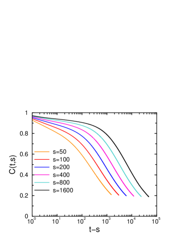
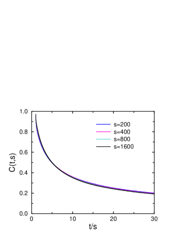
Figure 1: Two-time autocorrelator in the $2D$ Glauber-Ising model, with temperature $T=1.5=0.66T_{c}$ on a $600^{2}$ lattice and a disordered initial state.

In figure 1 we show the autocorrelator $C(t,s)$ of the $2D$ kinetic Ising model with Glauber dynamics after a quench to the final temperature $T=1.5$. In the left panel, the dependence of $C(t,s)$ on the time difference $\tau=t-s$ is shown. Clearly, the autocorrelator depends on both $t$ and $s$. For large values of $s$ and $\tau\lesssim s$, the values of $C(t,s)$ reach a quasistationary value $C_{\rm qs}(\tau)\simeq M_{\rm eq}^{2}$, where $M_{\rm eq}$ is the equilibrium magnetization. In the regime $\tau\gtrsim s$ one observes an algebraic decay of $C(t,s)$. Qualitatively similar behaviour is known from glassy systems and the simultaneous dependence of $C(t,s)$ and/or $R(t,s)$ on both $t$ and $s$ is the formal definition of ageing behaviour. The strong dependence of $C(t,s)$ on the waiting time (which expresses the sensibility of the system’s properties on its entire history) seems at first sight to lead to irreproducible data and hence to prevent a theoretical understanding of the ageing phenomenon. Remarkably, Struik Stru78 observed in polymeric glasses submitted to mechanical stress that the linear responses of quite distinct materials could be mapped onto a single and universal master curve. We illustrate this here in the ferromagnetic Glauber-Ising model through the data collapse in the right panel of figure 1. Remarkably, a dynamical scaling holds although the equilibrium state need not be scale-invariant.

On a more microscopic level, correlated domains of a linear size $L(t)$ form. These are ordered if $T<T_{c}$ but do contain internal long-range fluctuations at criticality. In the first case, the system undergoes phase-ordering kinetics and in the second non-equilibrium critical dynamics. For sufficiently large times, the domain size scales with time as

$$L(t)\sim t^{1/z}$$ (2)

where $z$ is the dynamical exponent. The slow relaxation to global equilibrium (although local equilibrium is rapidly achieved) comes about since for $T<T_{c}$ there are at least two distinct and competing equilibrium states. These states merge at $T=T_{c}$. On each site $\vec{r}$ the local environment selects the local equilibrium state.

As suggested from figure 1, one expects a scaling regime to occur when

$$t\gg\tau_{\rm micro}\;\;,\;\;s\gg\tau_{\rm micro}\;\;,\;\;t-s\gg\tau_{\rm micro}$$ (3)

where $\tau_{\rm micro}$ is some ‘microscopic’ time scale. We shall see later how important the third condition in (3) is. If the conditions (3) hold, one expects Bray94 ; Godr02

$$\halign to=433.62pt{\@eqnsel\hskip\@centering$\displaystyle{#}$&\global\@eqcnt\@ne\hskip 2\arraycolsep\hfil${#}$\hfil&\global\@eqcnt\tw@\hskip 2\arraycolsep$\displaystyle{#}$\hfil&\llap{#}\cr 0.0pt plus 1000.0pt$\displaystyle{C(t,s) &10.0pt\hfil${=&10.0pt$\displaystyle{s^{-b} f_{C}(t/s) \;\;\;\;\;\;, \;\; f_{C}(y)\sim y^{-\lambda_{C}/z} \;\; ; \;\; y\to\infty {}&\hbox to0.0pt{\hss{\rm(0.4a)}\cr\penalty 100\vskip 3.0pt\vskip 0.0pt\cr 0.0pt plus 1000.0pt$\displaystyle{R(t,s) &10.0pt\hfil${=&10.0pt$\displaystyle{s^{-1-a} f_{R}(t/s) \;\; , \;\; f_{R}(y)\sim y^{-\lambda_{R}/z} \;\; ; \;\; y\to\infty &\hbox to0.0pt{\hss{\rm(0.4b)}\cr}}}}}}}}}$$

These scaling forms should hold for both $T<T_{c}$ and $T=T_{c}$ although the values of the exponents will in general be different in these two cases. Here $\lambda_{C}$ and $\lambda_{R}$ are the autocorrelation Fish88 and autoresponse Pico02 exponents, respectively. They are independent of the equilibrium exponents and of $z$ Jans89 . It was taken for granted since a long time that $\lambda_{C}=\lambda_{R}$ but examples to the contrary have recently been found for spatial long-range correlations in the initial data Pico02 and in the random-phase sine-Gordon model Sche03 . If $T_{\rm ini}=\infty$, the inequality $\lambda_{C}=\lambda_{R}\geq d/2$ holds Yeun96 .

Table 1: Values of the non-equilibrium exponents $a$, $b$ and $z$ for non-conserved ferromagnets with $T_{c}>0$. The non-trivial critical-point value $z_{c}$ is model-dependent.

	$a$	$b$	$z$	Class
$T=T_{c}$	$(d-2+\eta)/z$	$(d-2+\eta)/z$	$z_{c}$	L
$T<T_{c}$	$(d-2+\eta)/z$	0	2	L
	$1/z$	0	2	S

The values of the non-equilibrium exponents $a$ and $b$ apparently depend on properties of the equilibrium system as follows Henk02a and are listed in table 1, together with those of $z$. We restrict to non-conserved ferromagnetic systems with $T_{c}>0$. If the equilibrium order parameter correlator $C_{\rm eq}(\vec{r})\sim\exp(-|\vec{r}|/\xi)$ with a finite $\xi$, the system is said to be of class S and if $C_{\rm eq}(\vec{r})\sim|\vec{r}|^{-(d-2+\eta)}$, it is said to be of class L. At criticality, a system is always in class L, but if $T<T_{c}$, systems such as the Glauber-Ising model are in class S, whereas the kinetic spherical model is in class L. For class S, the value of $a$ comes from the well-accepted idea Bert99 ; Bouc00 that the time-dependence of macroscopic averages comes from the motion of the domain walls. For class L, it follows from a hyperscaling argument Henk03e .

Having fixed the values of the critical exponents, we can state our main question: what can be said on the form of the universal scaling functions $f_{C}(y),f_{R}(y)$ in a general, model-independent way ?

2 Local scale-invariance

Our starting point is the rich evidence, accumulated through many decades and reviewed in Bray94 , in favour of dynamical scale-invariance in ageing phenomena. The order parameter field $\phi=\phi(t,\vec{r})$ scales

$$\phi(t,\vec{r})=\mathfrak{b}^{-x_{\phi}}\phi(\mathfrak{b}^{-z}t,\mathfrak{b}^{-1}\vec{r})$$ (5)

where $\mathfrak{b}$ is a constant rescaling factor. We now ask whether eq. (5) can be sensibly generalized to general space-time dependent rescalings $\mathfrak{b}=\mathfrak{b}(t,\vec{r})$ Henk94 ; Henk97 ; Henk02 . This ansatz can be motivated as follows.

Example 1. Consider an equilibrium critical point in $(1+1)$-dimensional space-time. Then $z=1$ and let $w=t+{\rm i}r$ and $\bar{w}=t-{\rm i}r$. Any angle-perserving space-time transformation is conformal and is given by the analytic transformations $w\mapsto f(w),\bar{w}\mapsto\bar{f}(\bar{w})$. A well-known result from field theory states Card96 that for short-ranged interactions, there is a Ward identity such that invariance under space- and time-translations, rotations and dilatations implies conformal invariance. Furthermore, basic quantities as the order parameter are primary under the conformal group and transform as $\phi(w,\bar{w})\mapsto(f^{\prime}(w)\bar{f}^{\prime}(\bar{w}))^{x_{\phi}/2}\phi(f(w)\bar{f}(\bar{w}))$ Bela84 . Hence $n$-point correlation functions and the values of the exponents $x_{\phi}$ can be found exactly from conformal symmetry, see e.g. Card96 ; Henk99 for introductions. Here we merely need the projective conformal transformations $f(w)=(\alpha w+\beta)/(\gamma w+\delta)$ with $\alpha\delta-\beta\gamma=1$. Fields which transform covariantly under those are called quasiprimary Bela84 . The associated infinitesimal transformations are $\ell_{n}=-w^{n+1}\partial_{w}$, $n\in\{\pm 1,0\}$, and satisfy the Lie algebra $[\ell_{n},\ell_{n^{\prime}}]=(n-n^{\prime})\ell_{n+n^{\prime}}$.

Example 2. Let $z=2$ and consider $d$ space dimensions. The Schrödinger group Sch($d$) is defined by Nied72

$$t\mapsto\frac{\alpha t+\beta}{\gamma t+\delta}\;\;,\;\;\vec{r}\mapsto\frac{{\cal R}\vec{r}+\vec{v}t+\vec{a}}{\gamma t+\delta}\;\;;\;\;\alpha\delta-\beta\gamma=1$$ (6)

where ${\cal R}\in SO(d)$, $\vec{a},\vec{v}\in\mathbb{R}^{d}$ and $\alpha,\beta,\gamma,\delta\in\mathbb{R}$. It is well-known that Sch($d$) is the maximal kinematic group of the free Schrödinger equation ${\cal S}\psi=0$ with ${\cal S}=2m{\rm i}\partial_{t}-\partial_{\vec{r}}^{2}$ Nied72 (that is, it maps any solution of ${\cal S}\psi=0$ to another solution). There are many Schrödinger-invariant systems, e.g. non-relativistic free fields Hage72 or the Euler equations of fluid dynamics ORai01 . As in the conformal case, for local theories there is a Ward identity such that Henk03

$$\left.\begin{array}[]{l}\mbox{\rm space translation invariance}\\ \mbox{\rm scale invariance with $z=2$}\\ \mbox{\rm Galilei invariance}\end{array}\right\}\Longrightarrow\mbox{\rm Schr\"{o}dinger invariance}$$ (7)

We point out that Galilei invariance has to be required and for applications to ageing we note that time-translation invariance is not needed. Indeed, a non-trivial Galilei-invariance is only possible for a complex wave function $\psi$. In applications to ageing, we shall identify below the ‘complex conjugate’ of the order parameter $\phi^{*}=\widetilde{\phi}$ with the response field of non-equilibrium field theory Henk03 . We denote the Lie algebra of Sch($d$) by $\mathfrak{sch}_{d}$. Specifically, $\mathfrak{sch}_{1}=\overline{\{X_{\pm 1,0},Y_{\pm 1/2},M_{0}\}}$ with the non-vanishing commutation relations

$$\left[X_{n},X_{n^{\prime}}\right] = (n-n^{\prime})X_{n+n^{\prime}}\;\;,\;\;\left[X_{n},Y_{m}\right]=\left(\frac{n}{2}-m\right)Y_{n+m}\;\;,\;\;$$ (8)

$$\left[Y_{1/2},Y_{-1/2}\right] = M_{0}$$ (9)

where $n,n^{\prime}\in\{\pm 1,0\}$ and $m\in\{\pm 1/2\}$.

Example 3. For a dynamical exponent $z\neq 2$, we construct infinitesimal generators of local scale transformations from the following requirements Henk02 (for simplicity, set $d=1$): (a) Transformations in time are $t\mapsto(\alpha t+\beta)/(\gamma t+\delta)$ with $\alpha\delta-\beta\gamma=1$. (b) The generator for time-translations is $X_{-1}=-\partial_{t}$ and for dilatations $X_{0}=-t\partial_{t}-z^{-1}r\partial_{r}-x/z$, where $x$ is the scaling dimension of the fields $\phi,\widetilde{\phi}$ on which the generators act. (c) Space-translation invariance is required, with generator $-\partial_{r}$. Starting from these conditions, we can show by explicit construction that there exist generators $X_{n}$, $n\in\{\pm 1,0\}$, and $Y_{m}$, $m=-1/z,1-1/z,\ldots$ such that

$$\left[X_{n},X_{n^{\prime}}\right]=(n-n^{\prime})X_{n+n^{\prime}}\;\;,\;\;\left[X_{n},Y_{m}\right]=\left(\frac{n}{z}-m\right)Y_{n+m}$$ (10)

For generic values of $z$, it is sufficient to specify the ‘special’ generator Henk02

$$X_{1}=-t^{2}\partial_{t}-Ntr\partial_{r}-Nxt-\widetilde{\alpha}r^{2}\partial_{t}^{N-1}-\widetilde{\beta}r^{2}\partial_{r}^{2(N-1)/N}-\widetilde{\gamma}\partial_{r}^{2(N-1)/N}r^{2}$$ (11)

from which all other generators can be recovered and where we wrote $z=2/N$ and $\widetilde{\alpha},\widetilde{\beta},\widetilde{\gamma}$ are free constants (further non-generic solutions exist for $N=1$ and $N=2$). For $z=2$ we recover the Schrödinger Lie algebra $\mathfrak{sch}_{1}$. Now, the condition $[X_{1},Y_{N/2}]=0$ is only satisfied if either (I) $\widetilde{\beta}=\widetilde{\gamma}=0$ which we call type I or else (II) $\widetilde{\alpha}=0$ which we call type II Henk02 .

Definition: If a system is invariant under the generators of either type I or type II it is said to be locally scale-invariant of type I or type II, respectively.

Local scale-invariance of type I can be used to describe strongly anisotropic equilibrium critical points. The application to Lifshitz points in $3D$ magnets with competing interactions is discussed in Plei01 ; Henk02 . The generators of type II are suitable for applications to ageing phenomena and will be studied here. First, we note that the generators $X_{n},Y_{m}$ form a kinematic symmetry of the linear differential equation ${\cal S}\psi=0$ where ${\cal S}=-z^{2}(\widetilde{\beta}+\widetilde{\gamma})\partial_{t}+\partial_{r}^{z}$ Henk02 . Recently, systems of non-linear equations invariant under these generators with $\widetilde{\alpha}=\widetilde{\beta}=\widetilde{\gamma}=0$ but extended to an infinite-dimensional symmetry $t\mapsto f(t)$ have been found Cher04 . Second, we consider the consequences for the scaling form of the response function $R(t,s;\vec{r})$. To do this, we recall that in the context of Martin-Siggia-Rose theory (see Jans92 ) a response function $R(t,s)=\langle\phi(t)\widetilde{\phi}(s)\rangle$ may be viewed as a correlator. If both $\phi$ and $\widetilde{\phi}$ transform as quasiprimaries, the hypothesis of covariance of the autoresponse function leads to the two conditions $X_{0}R=X_{1}R=0$. Of course, ageing systems cannot be invariant under time-translations. From the explicit form of the generators given above these equations are easily solved and the result can be compared with the expected asymptotic behaviour (1). This leads to the general result Henk01 ; Henk02

$$R(t,s)=r_{0}\Theta(t-s)\left(\frac{t}{s}\right)^{1+a-\lambda_{R}/z}\left(t-s\right)^{-1-a}$$ (12)

where $r_{0}$ is a normalization constant and the causality condition $t>s$ is explicitly included. Furthermore, the space-time response is given by $R(t,s;\vec{r})=R(t,s)\Phi\left(r(t-s)^{-1/z}\right)$ where $\Phi(u)$ solves the equation Henk02

$$\left[\partial_{u}+z\left(\widetilde{\beta}+\widetilde{\gamma}\right)u\partial_{u}^{2-z}+2z(2-z)\widetilde{\gamma}\partial_{u}^{1-z}\right]\Phi(u)=0$$ (13)

In the special case $z=2$, this reduces to Henk94

$$R(t,s;\vec{r})=R(t,s)\exp\left(-\frac{\cal M}{2}\frac{\vec{r}^{2}}{t-s}\right)$$ (14)

where ${\cal M}=\widetilde{\beta}+\widetilde{\gamma}$ is constant.

We point out that the derivation of the space-time response needs the assumption of Galilei-invariance (suitably generalized if $z\neq 2$). In turn, the confirmation of the form (14) is a given system undergoing ageing provides evidence in favour of Galilei-invariance in that system. We shall next describe tests of (12,14) in the Glauber-Ising model in $d\geq 2$ dimensions before we return to a fuller discussion of the physical origins of local scale-invariance.

3 Numerical test in the Glauber-Ising model

We wish to test the predictions (12,14) of local scale-invariance in the kinetic Glauber-Ising model, defined by the Hamiltonian ${\cal H}=-\sum_{(\vec{i},\vec{j})}\sigma_{\vec{i}}\sigma_{\vec{j}}$ where $\sigma_{\vec{i}}=\pm 1$. Based on a master equation, we use the heat-bath stochastic rule

$$\sigma_{\vec{i}}(t+1)=\pm 1\mbox{\rm~{}~{}with probability~{}}\frac{1}{2}\left[1\pm\tanh(h_{\vec{i}}(t)/T)\right]$$ (15)

with the local field $h_{\vec{i}}(t)=\sum_{\vec{n}(\vec{i})}\sigma_{\vec{n}}(t)$ and $\vec{n}(\vec{i})$ runs over the nearest neighbours of the site $\vec{i}$.

The response function is too noisy to be measured directly, therefore following Barr98 one may add a quenched spatially random magnetic field $\pm h_{(0)}$ between the times $t_{1}$ and $t_{2}$ and measure the integrated response $M(t,t_{1},t_{2}):=h_{(0)}\int_{t_{1}}^{t_{2}}\!\mathrm{d}u\,R(t,u)$. Two schemes a widely used, namely the ‘zero-field-cooling’ (ZFC) scheme, where $t_{1}=s$ and $t_{2}=t$ and the ‘thermoremanent’ (TRM) scheme, where $t_{1}=0$ and $t_{2}=s$. However, in both schemes it is not possible to naïvely use the scaling form (1) and integrate in order to obtain $M$. This comes about since in both cases some of the conditions (3) for the validity of this scaling form are violated. Taking this fact into account leads to the following results Henk02a ; Henk03e : (a) the thermoremanent magnetization

$$\rho(t,s) := \int_{0}^{s}\!\mathrm{d}u\,R(t,u)=r_{0}s^{-a}f_{M}(t/s)+r_{1}s^{-\lambda_{R}/z}g_{M}(t/s)$$ (16)

$$f_{M}(y) = y^{-\lambda_{R}/z}{{}_{2}F_{1}}\left(1+a,\frac{\lambda_{R}}{z}-a;\frac{\lambda_{R}}{z}-a+1;\frac{1}{y}\right)\;,\;\;g_{M}(y)\simeq y^{-\lambda_{R}/z}$$ (17)

where $r_{0,1}$ are normalization constants. The first term is as expected from naïve scaling. In practice, $a$ and $\lambda_{R}/z$ are often quite close and the size of the correction term may well be notable for $T<T_{c}$ (at $T=T_{c}$, $a$ and $\lambda_{R}/z$ are usually quite distinct); (b) the zero-field-cooled susceptibility

$$\chi(t,s):=\int_{s}^{t}\!\mathrm{d}u\,R(t,u)=\chi_{0}+s^{-A}g(t/s)+{\rm O}\left(s^{-a}\right)$$ (18)

with a constant $\chi_{0}$ and some scaling function $g$. For systems of class S, we have $A=a-\kappa$, where $\kappa$ measures the width $w(t)\sim t^{\kappa}$ of the domain walls Henk03e . In the Glauber-Ising model, one has $\kappa=1/4$ in $2D$ and $w(t)\sim\sqrt{\ln t\,}$ in $3D$ Abra89 , while $\kappa=0$ for $d>3$. Consequently, the term of order $s^{-a}$ coming from naïve scaling is not even the dominant one in the long-time limit $s\to\infty$ and a simple phenomenological analysis of data of $\chi(t,s)$ is likely to produce misleading results. For systems of class L, $A=0$.

Indeed, based on high-quality numerical MC data for $\chi(t,s)$ in the $2D$ Glauber-Ising model and performing a straightforward scaling analysis according to $\chi(t,s)\sim s^{-a}$ but without taking the third condition (3) for the validity of scaling into account, it had been claimed that $a=1/4$ in that model Corb03 . However, that analysis is based on the identification $A\stackrel{{\scriptstyle?}}{{=}}a$ which cannot be maintained. Rather, for the $2D$ Glauber-Ising model, one has $a=1/2$ and $\kappa=1/4$, reproducing $A=1/4$ in agreement with the MC data.

Table 2: Values of the autoresponse exponent $\lambda_{R}$ and of the parameters $r_{0}$, $r_{1}$ and $\cal M$ in the Glauber-Ising model for an infinite-temperature initial state.

$d$	$T$	$\lambda_{R}$	$r_{0}$	$r_{1}$	$\cal M$
2	1.5	1.26	$~{}~{}~{}1.76\pm 0.03$	$-1.84\pm 0.03$	$4.08\pm 0.04$
3	3	1.60	$~{}~{}~{}0.10\pm 0.01$	$~{}~{}\,0.20\pm 0.01$	$4.22\pm 0.05$

After these preparations, we can now present numerical Monte Carlo (MC) data and compare them with the predictions (12,14). We consider the thermoremanent magnetization $\rho(t,s)$ and subtract off the leading finite-time correction according to (16). For $T<T_{c}$ this leads to the parameter values collected in table 2, see Henk03b for details. Then the MC data both at $T=T_{c}$ and for $T<T_{c}$ for $\rho(t,s)$ are in full agreement with (16) Henk01 ; Henk03b , in both $2D$ and $3D$. Here we present a direct test of Galiliei-invariance by considering the space-time integrated response

$$\frac{\mathrm{d}\rho(t,s;\mu)}{\mathrm{d}\Omega}=T\int_{0}^{s}\!\mathrm{d}u\int_{0}^{\sqrt{\mu s\,}}\!\mathrm{d}r\,r^{d-1}R(t,u;\vec{r})=r_{0}s^{d/2-a}\rho^{(2)}(t/s,\mu)$$ (19)

with an explicitly known expression for $\rho^{(2)}$ following from (14) and the leading finite-time correction is already subtracted off Henk03b . Since all non-universal parameters were determined before and are listed in table 2, this comparison between simulation and local scale-invariance is parameter-free. The result in shown in figure 2 in $2D$ and we find a perfect agreement. A similar results holds in $3D$ Henk03b .

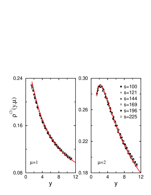
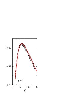
Figure 2: Integrated space-time response of the $2D$ Glauber-Ising model. After Henk03b .

This direct evidence in favour of Galilei-invariance in the phase-ordering kinetics of the Glauber-Ising model is all the more remarkable since the zero-temperature time-dependent Ginzburg-Landau equation (TDGL), which is usually thought to describe the same system (e.g. Bray94 ), does not have this symmetry. Indeed a recent second-order result for $R(t,s)$ does not agree with (12) Maze04 (similar corrections also arise at $T=T_{c}$ Cala03 ). On the other hand, $\lambda_{C}=1$ from the exact solution of the $1D$ Glauber-Ising model at $T=0$ Godr02 , while $\lambda_{C}\simeq 0.6006\ldots$ in the $1D$ TDGL Bray95 , implying that these two models belong to distinct universality classes.

Confirmations of (12,14) in exactly solvable models are reviewed in Henk02 .

4 Influence of noise

We now wish to review the present state of theoretical arguments Henk03 ; Pico04 in order to understand from where the recent numerical evidence in favour of a larger dynamical symmetry than mere scale-invariance in ageing phenomena might come from. We shall do this here for phase-ordering kinetics. Then $z=2$ and we have to consider the Schrödinger group and Schrödinger-invariant systems. For simplicity, we often set $d=1$. From the following discussion, the importance of Galilei-invariance will become clear, see also (7).

A) Consider the free Schrödinger equation $(2{\cal M}\partial_{t}-\partial_{r}^{2})\phi=0$ where ${\cal M}={\rm i}m$ is fixed. While an element of the Schrödinger group acts projectively (i.e. up to a known companion function Nied72 ) on the wave function $\phi$, we can go over to a true representation by treating $\cal M$ as an additional variable. Following Giul96 , we define a new coordinate $\zeta$ and a new wave function $\psi$ by

$$\phi(t,r)=\frac{1}{\sqrt{2\pi}}\int_{\mathbb{R}}\!{\rm d}\zeta\,e^{-{\rm i}{\cal M}\zeta}\psi(\zeta,t,r)$$ (20)

We denote time $t$ as the zeroth coordinate and $\zeta$ as coordinate number $-1$.

We inquire about the maximal kinematic group in this case Henk03 . Now, the projective phase factors can be absorbed into certain translations of the variable $\zeta$ Henk03 . Furthermore, the free Schrödinger equation becomes

$$\left(2{\rm i}\partial_{\zeta}\partial_{t}+\partial_{r}^{2}\right)\psi(\zeta,t,r)=0$$ (21)

In order to find the maximal kinematic symmetry of this equation, we recall that the three-dimensional Klein-Gordon equation $\sum_{\mu=-1}^{1}\partial_{\mu}\partial^{\mu}\Psi(\vec{\xi})=0$ has the $3D$ conformal algebra $\mathfrak{conf}_{3}\cong so(4,1)$ as maximal kinematic symmetry. By making the following change of variables

$$\zeta=\left(\xi_{0}+{\rm i}\xi_{-1}\right)/2\;\;,\;\;t=\left(-\xi_{0}+{\rm i}\xi_{-1}\right)/2\;\;,\;\;r=\xi_{1}\sqrt{{\rm i}/2}$$ (22)

and setting $\psi(\zeta,t,r)=\Psi(\vec{\xi})$, the $3D$ Klein-Gordon equation reduces to (21). Therefore, for variable masses $\cal M$, the maximal kinematic symmetry algebra of the free Schrödinger equation in $d$ dimensions is isomorphic to the conformal algebra $\mathfrak{conf}_{d+2}$ and we have the inclusion of the complexified Lie algebras $(\mathfrak{sch}_{d})_{\mathbb{C}}\subset(\mathfrak{conf}_{d+2})_{\mathbb{C}}$ Henk03 ; Burd73 .

B) The Galilei-invariance of the free Schrödinger equation requires the existence of a formal ‘complex conjugate’ $\phi^{*}$ of the order parameter $\phi$. On the other hand, a common starting point in the description of ageing phenomena is a Langevin equation which may be turned into a field theory using the Martin-Siggia-Rose (MSR) formalism Jans92 ; Card96 and which involves besides $\phi$ the response field $\widetilde{\phi}$. If we identify $\phi^{*}=\widetilde{\phi}$ and use (20) together with the assumption that $\psi$ is real to define the complex conjugate, then the causality condition that

$$R(t,s;\vec{r})=\langle\phi(t,\vec{r})\widetilde{\phi}(s,\vec{0})\rangle=\langle\phi(t,\vec{r})\phi^{*}(s,\vec{0})\rangle$$ (23)

vanishes for $t<s$, follows naturally (and similarly for three-point response functions) Henk03 . Therefore, the calculation of response and of correlation functions from a dynamical symmetry should be done in the same way.

C) So far, we have concentrated exclusively in applications of local scale-invariance to finding the form of response functions while the determination of correlation functions was not yet adressed. We shall do so now and consider the Langevin equation (with $D^{-1}=2{\cal M}$) Pico04

$$\partial_{t}\phi=-D\frac{\delta{\cal H}}{\delta\phi}-Dv(t)\phi+\eta$$ (24)

where $\cal H$ is the usual Ginzburg-Landau functional, $v(t)$ is a time-dependent Lagrange multiplier which will be chosen to produce the constraint $C(t,t)=1$ and $\eta$ is an uncorrelated gaussian noise describing the coupling to a heat bath such that $\langle\eta\rangle=0$ and $\langle\eta(t,\vec{r})\eta(t^{\prime},\vec{r}^{\prime})\rangle=2DT\delta(t-t^{\prime})\delta(\vec{r}-\vec{r}^{\prime})$. Another source of noise comes from the initial conditions and we shall always use an uncorrelated initial state such that

$$C(0,0;\vec{r})=\langle\phi(0,\vec{r})\phi(0,\vec{0})\rangle=a_{0}\delta(\vec{r})$$ (25)

where $a_{0}$ is a constant.

The MSR action of (24) reads $S[\phi,\widetilde{\phi}]=S_{0}[\phi,\widetilde{\phi}]+S_{b}[\phi,\widetilde{\phi}]$ where

$$\halign to=433.62pt{\@eqnsel\hskip\@centering$\displaystyle{#}$&\global\@eqcnt\@ne\hskip 2\arraycolsep\hfil${#}$\hfil&\global\@eqcnt\tw@\hskip 2\arraycolsep$\displaystyle{#}$\hfil&\llap{#}\cr 0.0pt plus 1000.0pt$\displaystyle{S_{0}[\phi,\widetilde{\phi}] &10.0pt\hfil${=&10.0pt$\displaystyle{\int\!\mathrm{d}t \mathrm{d}\vec{r}\> \widetilde{\phi} \left( \frac{\partial\phi}{\partial t} +D\frac{\delta{\cal H}}{\delta\phi} + Dv(t)\phi\right) {}&\hbox to0.0pt{\hss{\rm(0.26a)}\cr\penalty 100\vskip 3.0pt\vskip 0.0pt\cr 0.0pt plus 1000.0pt$\displaystyle{S_{b}[\phi,\widetilde{\phi}] &10.0pt\hfil${=&10.0pt$\displaystyle{-DT\int\!\mathrm{d}t \mathrm{d}\vec{r}\> \widetilde{\phi}(t,\vec{r})^{2} - \frac{a_{0}}{2} \int\!\mathrm{d}\vec{r}\> \widetilde{\phi}(0,\vec{r})^{2} &\hbox to0.0pt{\hss{\rm(0.26b)}\cr}}}}}}}}}$$

and we used (25), see Maze04 . Here $S_{0}$ describes the noiseless part of the action while the thermal and the initial noise are contained in $S_{b}$. Finally, the potential $v(t)$ can be absorbed into a gauge transformation; for example if $\phi^{(0)}$ is a solution of the free Schrödinger equation, then $\phi=\phi^{(0)}k(t)$ solves the Schrödinger equation with the potential $v(t)$ and where

$$k(t):=\exp\left(-D\int^{t}\!\mathrm{d}u\>v(u)\right)$$ (27)

The realization of the Schrödinger algebra with $v(t)\neq 0$ is easily found Pico04 .

We now assume in addition to dynamical scaling that $\cal H$ is such that at temperature $T=0$, the theory is Galilei-invariant Pico04 . This looks physically reasonable and we now explore some consequences of this hypothesis. We denote by $\langle\cdot\rangle_{0}$ an average carried out using only the noiseless part $S_{0}$ of the action. The Bargman superselection rules state that $\langle\underbrace{\phi\cdots\phi}_{n}\underbrace{\widetilde{\phi}\cdots\widetilde{\phi}}_{m}\rangle_{0}=0$ if $n\neq m$. First, the response function is

$$R(t,s;\vec{r}) = \left\langle\phi(t,\vec{r})\widetilde{\phi}(s,\vec{0})\right\rangle=\left\langle\phi(t,\vec{r})\widetilde{\phi}(s,\vec{0})\exp\left(-S_{b}[\phi,\widetilde{\phi}]\right)\right\rangle_{0}$$ (28)

$$= \left\langle\phi(t,\vec{r})\widetilde{\phi}(s,\vec{0})\right\rangle_{0}=:R_{0}(t,s;\vec{r})$$ (29)

where in the last line the exponential was expanded and the Bargman superselection rule was used. Here $R_{0}$ is the noiseless response and the form (12,14) of Schrödinger-invariance is recovered if $v(t)=(2{\cal M})(1+a-\lambda_{R}/2)t^{-1}$ Pico04 . In other words, under the stated hypothesis, the response function is independent of the noises. This is certainly in agreement with the explicit model calculations reviewed in section 3.

Second, we now obtain the autocorrelation function. As before Pico04

$$C(t,s) = \left\langle\phi(t,\vec{r})\phi(s,\vec{r})\exp\left(-S_{b}[\phi,\widetilde{\phi}]\right)\right\rangle_{0}$$ (30)

$$= DT\int\!\mathrm{d}u\mathrm{d}\vec{R}\,R_{0}^{(3)}(t,s,u;\vec{R})+\frac{a_{0}}{2}\int\!\mathrm{d}\vec{R}\,R_{0}^{(3)}(t,s,0;\vec{R})$$ (31)

where $R_{0}^{(3)}(t,s,u;\vec{R})=\langle\phi(t,\vec{y})\phi(s,\vec{y})\widetilde{\phi}(u,\vec{R}+\vec{y})^{2}\rangle_{0}$. In contrast with the response function, the autocorrelation function contains only noisy terms and in fact vanishes in the absence of noise. By hypothesis, Schrödinger-invariance holds for the noiseless theory and the three-point function $R_{0}^{(3)}$ is fixed up to a scaling function of a single variable Henk94 ; Pico04 .

Working out the asymptotic behaviour of $C(t,s)$ for $y=t/s\to\infty$ according to (1) and comparing with the response function (29), we find that for any coarsening system with a disordered initial state (25) and whose noiseless part is Schrödinger-invariant, the relation $\lambda_{C}=\lambda_{R}$ holds true Pico04 . For the first time a general sufficient criterion for this exponent relation is found.

The autocorrelator scaling function becomes for phase-ordering

$$f_{C}(y)=\frac{a_{0}}{2}y^{\lambda_{C}/2}(y-1)^{-\lambda_{C}}\Phi\left(\frac{y+1}{y-1}\right)$$ (32)

but the scaling function $\Phi(w)$ is left undetermined by Schrödinger-invariance. If in addition we require that $C(t,s)$ should be non-singular at $t=s$, the asymptotic behaviour $\Phi(w)\sim w^{-\lambda_{C}}$ for $w\to\infty$ follows. Provided that form should hold true for all values of $w$, we would obtain approximately

$$f_{C}(y)\approx f_{0}\left(\frac{(y+1)^{2}}{4y}\right)^{-\lambda_{C}/2}$$ (33)

Indeed, this is found to be satisfied for several ageing spin systems with an underlying free-field theory Pico04 . On the other hand, (33) does not hold true in the Glauber-Ising model. Work is presently being carried out in order to describe $f_{C}(y)$ in this model and will be reported elsewhere Henk04 .

It is a pleasure to thank M. Pleimling, A. Picone and J. Unterberger for the fruitful collaborations which led to the results reviewed here. This work was supported by CINES Montpellier (projet pmn2095) and by the Bayerisch-Französisches Hochschulzentrum (BFHZ).

References

- (1) L.C.E. Struik: Physical ageing in amorphous polymers and other materials (Elsevier, Amsterdam 1978).
- (2) A.J. Bray: Adv. Phys. 43, 357 (1994).
- (3) J.P. Bouchaud in M.E. Cates, M.R. Evans (eds) Soft and fragile matter (IOP Press, Bristol 2000).
- (4) C. Godrèche, J.M. Luck: J. Phys. Cond. Matt. 14, 1589 (2002).
- (5) L.F. Cugliandolo: in Slow Relaxation and non equilibrium dynamics in condensed matter, Les Houches Session 77 July 2002, J-L Barrat, J Dalibard, J Kurchan, M V Feigel’man eds (Springer, Heidelberg 2003)
- (6) D.S. Fisher, D.A. Huse: Phys. Rev. B38, 373 (1988).
- (7) A. Picone, M. Henkel: J. Phys. A35, 5575 (2002).
- (8) H.K. Janssen, B. Schaub, B. Schmittmann: Z. Phys. B73, 539 (1989).
- (9) G. Schehr, P. Le Doussal: Phys. Rev. E68, 046101 (2003).
- (10) C. Yeung, M. Rao, R.C. Desai: Phys. Rev. E53, 3073 (1996).
- (11) M. Henkel, M. Paeßens, M. Pleimling: Europhys. Lett. 62, 644 (2003)
- (12) L. Berthier, J.L. Barrat, and J. Kurchan: Eur. Phys. J. B11, 635 (1999).
- (13) M. Henkel, M. Paeßens, M. Pleimling: cond-mat/0310761.
- (14) M. Henkel: J. Stat. Phys. 75, 1023 (1994).
- (15) M. Henkel: Phys. Rev. Lett. 78, 1940 (1997).
- (16) M. Henkel: Nucl. Phys. B641, 405 (2002).
- (17) J.L. Cardy: Scaling and Renormalization in Statistical Mechanics (Cambridge University Press, Cambridge 1996).
- (18) A.A. Belavin, A.M. Polyakov, A.B. Zamolodchikov: Nucl. Phys. B241, 333 (1984).
- (19) M. Henkel: Phase Transitions and Conformal Invariance (Springer, Heidelberg 1999).
- (20) U. Niederer: Helv. Phys. Acta 45, 802 (1972).
- (21) C.R. Hagen: Phys. Rev. D5, 377 (1972).
- (22) L. O’Raifeartaigh and V.V. Sreedhar: Ann. of Phys. 293, 215 (2001).
- (23) M. Henkel, J. Unterberger: Nucl. Phys. B660, 407 (2003).
- (24) M. Pleimling, M. Henkel: Phys. Rev. Lett. 87, 125702 (2001).
- (25) R. Cherniha, M. Henkel: math-ph/0402059.
- (26) H.K. Janssen: in G. Györgyi et al. (eds) From Phase transitions to Chaos, World Scientific (Singapour 1992), p. 68
- (27) M. Henkel, M. Pleimling, C. Godrèche, J.-M. Luck: Phys. Rev. Lett. 87, 265701 (2001).
- (28) A. Barrat: Phys. Rev. E57, 3629 (1998).
- (29) D.B. Abraham and P.J. Upton, Phys. Rev. B39, 736 (1989).
- (30) F. Corberi, E. Lippiello, M. Zannetti: Phys. Rev. E68, 046131 (2003).
- (31) M. Henkel, M. Pleimling: Phys. Rev. E68, 065101(R) (2003).
- (32) G.F. Mazenko: Phys. Rev. E69, 016114 (2004).
- (33) P. Calabrese, A. Gambassi: Phys. Rev. E67, 036111 (2003).
- (34) A.J. Bray, B. Derrida: Phys. Rev. E51, R1633 (1995).
- (35) A. Picone, M. Henkel: cond-mat/0402196.
- (36) D. Giulini: Ann. of Phys. 249, 222 (1996).
- (37) G. Burdet, M. Perrin, P. Sorba: Comm. Math. Phys. 34, 85 (1973).
- (38) M Henkel, A. Picone, M. Pleimling: to be published.