On universality in ageing ferromagnets

Abstract

This work is a contribution to the study of universality in out-of-equilibrium lattice models undergoing a second-order phase transition at equilibrium. The experimental protocol that we have chosen is the following: the system is prepared in its high-temperature phase and then quenched at the critical temperature $T_{c}$. We investigated by mean of Monte Carlo simulations two quantities that are believed to take universal values: the exponent $\lambda/z$ obtained from the decay of autocorrelation functions and the asymptotic value $X_{\infty}$ of the fluctuation-dissipation ratio $X(t,s)$. This protocol was applied to the Ising model, the 3-state clock model and the 4-state Potts model on square, triangular and honeycomb lattices and to the Ashkin-Teller model at the point belonging at equilibrium to the 3-state Potts model universality class and to a multispin Ising model and the Baxter-Wu model both belonging to the 4-state Potts model universality class at equilibrium.

1 Introduction

Universality is an extremely fruitful concept in statistical physics and has been widely studied in the context of systems undergoing a second order phase transition. At thermodynamic equilibrium, the length scale $\xi$ of spatial correlation functions of the local order parameter diverges as a power-law with a critical exponent $\nu$ as the temperature approaches the critical temperature. Other observables (energy, magnetisation, $\ldots$) display such a power-law dependence as well but with different critical exponents. It turns out that many microscopic details of the Hamiltonian do not change the value of these critical exponents. The big success of the renormalisation group has been to explain that a few number of these critical exponents are independent and that different models have the same set of critical exponents if they differ only by irrelevant operators. Consequently, the usual models of statistical physics can be classified into universality classes according to the value of their critical exponents. The space and order parameter dimensions, the Hamiltonian symmetries, the presence of long-range interactions, of randomness $\ldots$ determine the universality class. Not only critical exponents but also ratios of critical amplitudes turn out to be universal.

The question of universality in out-of-equilibrium processes has been addressed in the context of dynamical transitions undergone by reaction-diffusion systems [1]. A set of exponents can be defined, for instance using the algebraic decay with time of the density of active sites.

In the following, we will restrict ourselves to another important set of out-of-equilibrium processes provided by systems that undergo a second-order phase transition at equilibrium and that are quenched from their high-temperature phase to their critical point or their low-temperature phase. Because of the competition of domains in different equilibrium states, such systems never reach equilibrium in the thermodynamic limit [2]. The hypothesis was made that systems belonging to the same universality class at equilibrium share universal quantities if their time-evolution is governed by dynamics satisfying the same conservation laws and if order parameter and conserved quantities are related in the same way [3]. In the following, we will consider systems belonging to the same universality class at equilibrium and whose dynamics has no conserved quantity (model A). In this context new exponents have been defined: the dynamical exponent $z$ related to the growth of the domain length scale $L(t)$ with time by [3]

$$L(t)\sim t^{1/z}$$ (1)

and the autocorrelation exponent $\lambda$ related to the decay of two-time autocorrelation functions of the local order parameter [4, 5] by

$$C(t,s)\sim t^{-\lambda/z}.$$ (2)

These two new exponents $z$ and $\lambda$ take different values whether the system is quenched at its critical temperature $T_{c}$ or below. They are believed to be universal. Numerical calculations for the Ising model on square, triangular and honeycomb lattices [6] or for three different models belonging to the Ising equilibrium universality class [7] support this conjecture for the exponent $z$ at $T=T_{c}$. Simulations for other models, for instance the 3-state Potts model [8], give estimate for $z$ sufficiently close to give support to the conjecture of a dynamic universality.

The decay of persistence, i.e. the probability that the total order parameter has not changed sign at time $t$, defines a third new non-trivial exponent $\theta^{\prime}$. In the rather unusual case where the dynamics of the total order parameter is Markovian, it is related to the two previously-defined ones by $z\theta^{\prime}=\lambda-d+1-\eta/2$ [9].

Renormalisation-group study of the $O(n)$ model in $d=4-\epsilon$ dimension shows that if the system is quenched at the critical temperature from an initial state with a small non-vanishing magnetisation, the latter first grows as $t^{\theta}$ before decaying asymptotically as $\xi^{-\beta/\nu}\sim L(t)^{-\beta/\nu}\sim t^{-\beta/\nu z}$ [10]. The initial-slip critical exponent $\theta$ is related to the autocorrelation exponent by

$$\lambda=d-z\theta$$ (3)

where $d$ is the dimension of the space. This behaviour of the magnetisation has been exploited in the so-called short-time dynamics Monte Carlo method [11]. The question of universality has been addressed by several authors in this context. The Ashkin-Teller model has been studied by short-time dynamics for several points of its exactly-known critical line [12]. Unfortunately, the point belonging to the 3-state Potts model universality class, i.e. $y=3/4$ where $\nu={2-y\over 3-2y}$, has not been considered. Noting that the estimates of $\theta$ given by the authors vary roughly linearly with the parameter $y$, one can estimate the exponent $\theta$ at the point $y=3/4$ to be $\theta\simeq 0.111$. This result is not compatible with that obtained for the 3-state Potts model [8]: $\theta\simeq 0.0815(27)$. Moreover, numerical estimates of this exponent $\theta$ for the Baxter-Wu [13] and a multispin Ising model [14] both belonging to the 4-state Potts model equilibrium universality class are incompatible with estimates for the latter while the dynamical exponent $z$ seems to be the same [13].

Apart from exponents, ratios of amplitudes have also been conjectured to be universal, as for example the fluctuation-dissipation ratio $X(t,s)$ in the asymptotic limit $t,s\rightarrow+\infty$. The response function $R(t,s)$ to an infinitesimal field $h(s)$ coupled to the local order parameter is expected to decay algebraically with time with the same exponent $\lambda/z$ as autocorrelation functions provided the initial state does not display spatial correlations. Note that autocorrelation and response functions are related at equilibrium by the fluctuation-dissipation theorem (FDT):

$$k_{B}T\ \!R(t,s)={\partial\over\partial s}C(t,s).$$ (4)

On the basis of a mean-field study of a spin-glass-like model, it was conjectured that the fluctuation-dissipation theorem may be generalised by adding to Eq. 4 a multiplicative factor depending on time only through autocorrelation functions [15]:

$$k_{B}T\ \!R(t,s)\sim X\big{[}C(t,s)\big{]}{\partial\over\partial s}C(t,s),\quad(t\sim s\gg 1).$$ (5)

However, numerical simulations for the Ising model [16] and renormalisation-group calculations for the $O(n)$ model [17] suggest that the fluctuation-dissipation ratio is not a function of $C(t,s)$ only but of $t/s$. Scaling arguments constrain the autocorrelation and response function to the following asymptotic behaviour [18] at $T_{c}$:

$$C(t,s)\sim s^{-{2\beta\over\nu z}}f_{C}\left({t\over s}\right),\quad k_{B}T_{c}\ \!R(t,s)\sim s^{-1-{2\beta\over\nu z}}f_{R}\left({t\over s}\right)\quad(t\sim s\gg 1)$$ (6)

where both $f_{C}(x)$ and $f_{R}(x)$ are scaling functions whose asymptotic behaviour is given by

$$f_{C/R}(x)\sim A_{C/R}\ \!x^{-\lambda/z},\quad x\rightarrow+\infty.$$ (7)

Inserting Eq. 6 and 7 into Eq. 5 leads to the asymptotic value of the fluctuation-dissipation ratio:

$$X_{\infty}=\lim_{t,s\rightarrow+\infty}X(t,s)={A_{R}\over A_{C}}\left[{\lambda\over z}-{2\beta\over\nu z}\right]^{-1}$$ (8)

which turns out to depend only on exponents which are believed to be universal and on the ratio of autocorrelation and response amplitudes. The latter has been conjectured to be universal [18]. This conjecture applies thus to $X_{\infty}$ as well. Renormalisation-group calculations [17] of the $O(1)$ model gives indeed an estimate of $X_{\infty}$ compatible with numerical values for the Ising model [19, 16, 21]. Moreover, a recent numerical calculation of the integrated response function to an exchange coupling perturbation gave an estimate of $X_{\infty}$ in full agreement with theses values [19]. The Ising model may be peculiar since a one-loop renormalisation-group calculation of the $O(1)$ model gives the same value of $X_{\infty}$ whether the order parameter is coupled to a conserved quantity (model C) or not (model A) [20]. Let us mention that calculations for the Ising-Glauber chain indicates that $X_{\infty}$ takes a non-vanishing value only with a well defined protocol : a quench at the critical temperature from an initial state with an infinite number of domain walls, i.e. from an initial disordered state [22].

The plan of this paper is the following: in the first section, the expressions of the Hamiltonians of the different models we studied are given. The Glauber dynamics is then defined and we review the method we used to calculate the fluctuation-dissipation ratio without resorting to the Cugliandolo conjecture (Eq 5). The second section is devoted to the characterisation of the three universality classes under consideration. The question of the influence of the lattice on the quantities that are supposed to be universal is addressed in the third section. The fourth section is devoted to the comparison of these universal quantities for different models belonging to the same universality class at equilibrium.

2 Dynamics and Models

2.1 Definition of the models

We have considered two-dimensional lattice models belonging at equilibrium to three different universality classes. The first of them is the Ising model [23] defined by the Hamiltonian:

$${\cal H}_{\rm Ising}=-J\sum_{(i,j)}\sigma_{i}\sigma_{j}-\sum_{i}h_{i}\sigma_{i},\quad\sigma_{i}=\pm 1$$ (9)

where the first sum extends to nearest neighbours on the lattice. A local magnetic field coupled to the local order parameter $m_{i}=\sigma_{i}$ has been added to allow for the definition of a response function. For vanishing magnetic field, the model undergoes a second-order phase transition associated to the breaking of a $Z(2)$-symmetry. Duality relation leads to the critical point on the square lattice $\beta_{c}J={1\over 2}\ln(1+\sqrt{2})$ where $\beta_{c}=1/k_{B}T_{c}$ [24]. Although triangular and honeycomb lattices are not self-dual but dual of each other, the exact determination of the critical temperature is nevertheless possible [25] and gives $\beta_{c}J\simeq 0.2746$ on a triangular lattice and $\beta_{c}J\simeq 0.6585$ on the honeycomb lattice.

The second universality class we have considered is that of the 3-state Potts model [26] whose Hamiltonian is

$${\cal H}_{\rm Potts}=-J\sum_{(i,j)}\delta_{\sigma_{i},\sigma_{j}}-\sum_{i}h_{i}\delta_{\sigma_{i},0},\quad\sigma_{i}=0,\ldots q-1$$ (10)

where the number of state $q$ is set to $q=3$. For vanishing magnetic field, the model undergoes a second-order phase transition associated to the breaking of a $Z(3)$-symmetry. Self-duality relation allows for the exact determination of the critical point: $\beta_{c}J=\ln(1+\sqrt{q})$ at zero-magnetic field on the square lattice. Critical points can also be obtained for the triangular and honeycomb lattices [25]. In order to achieve better numerical stability, we used an equivalent formulation of this model, known as the clock model, whose order parameter is vanishing at the critical temperature without resorting to any additional normalisation:

$${\cal H}_{\rm Clock}= - J\sum_{(i,j)}\cos\left({2\pi\over q}(\sigma_{i}-\sigma_{j})\right)$$ (11)

$$- \sum_{i}\left[h_{i}^{x}\cos\left({2\pi\over q}\sigma_{i}\right)+h_{i}^{y}\sin\left({2\pi\over q}\sigma_{i}\right)\right]\quad\sigma_{i}=0,\ldots q-1.$$

The critical temperature is readily obtained to be two-third of that of the equivalent $q$-state Potts model. As a prototype of model belonging to this universality class, we have chosen the Ashkin-Teller model [27] defined by the Hamiltonian

$${\cal H}_{\rm AT}=-J\sum_{(i,j)}\sigma_{i}\sigma_{j}-J^{\prime}\sum_{(i,j)}\tau_{i}\tau_{j}-K\sum_{(i,j)}\sigma_{i}\sigma_{j}\tau_{i}\tau_{j}-\sum_{i}h_{i}\sigma_{i},\quad\sigma_{i},\tau_{i}=\pm 1.$$ (12)

Indeed, in the isotropic case $J=J^{\prime}$ the universality class changes from that of the Ising model to that of the 4-state Potts model along an exactly-known critical line. The point belonging to the 3-state Potts model is defined by the critical couplings: $\beta_{c}J=\beta_{c}J^{\prime}\simeq 0.34763$ and $\beta_{c}K\simeq 0.14209$ [28].

The third universality class we have considered is that of the 4-state Potts model. For vanishing magnetic field, the model undergoes a second-order phase transition associated to the breaking of a $Z(4)$-symmetry. Duality relations allows for the determination of the critical point on the square, triangular and honeycomb lattices [25]. Apart from the 4-state Potts model, we have made calculations for two other models belonging to this universality class: the Baxter-Wu model [29] defined by the Hamiltonian

$${\cal H}_{\rm BW}=-J\sum_{(i,j,k)}\sigma_{i}\sigma_{j}\sigma_{k}-\sum_{i}h_{i}\sigma_{i},\quad\sigma_{i}=\pm 1$$ (13)

where the sum extend over all triangles of a triangular lattice and a multispin Ising model [30] defined on a square lattice by the Hamiltonian

$${\cal H}_{\rm DT}=-J\sum_{(i,j)}^{\prime}\sigma_{i}\sigma_{j}-K\sum_{(i,j,k)}^{\prime\prime}\sigma_{i}\sigma_{j}\sigma_{k}-\sum_{i}h_{i}\sigma_{i},\quad\sigma_{i}=\pm 1$$ (14)

where the first sum extends over couples of neighbour spins along the horizontal direction and the second over triplets of spins aligned along the vertical direction. For the Baxter-Wu model, the ground states correspond to spin configurations where triangle vertices are decorated with spins $\{+,+,+\}$, $\{+,-,-\}$, $\{-,+,-\}$ or $\{-,-,+\}$. In the case of the multispin Ising model, the ground-states correspond to rows decorated with the sequence of spins: $\{+,+,+\}$, $\{+,-,-\}$, $\{-,+,-\}$ or $\{-,-,+\}$. Duality relations lead for the Baxter-Wu model to the critical point $\beta_{c}J\simeq{1\over 2}\ln(1+\sqrt{2})$ and for the multispin Ising model to the same critical line in the $J-K$ plane than the anisotropic Ising model [30] from which we have chosen the point $\beta_{c}J=1$, $\beta_{c}K\simeq 0.1362$.

2.2 Glauber dynamics and observables

The time evolution of all these models is governed by the same discrete-time Glauber dynamics. Let us denote by $\wp(\{\sigma\},t)$ the probability of the spin configuration $\{\sigma\}$ at time $t$. The dynamics is defined by the usual master equation for Monte Carlo simulations:

$$\wp(\{\sigma\},t+1)=\sum_{\{\sigma^{\prime}\}}W(\{\sigma^{\prime}\}\rightarrow\{\sigma\},t)\wp(\{\sigma^{\prime}\},t)$$ (15)

where $W(\{\sigma\}\rightarrow\{\sigma^{\prime}\},t)$ is the transition rate per time step from the state $\{\sigma\}$ to the state $\{\sigma^{\prime}\}$ at time $t$. The conditional probability $\wp(\{\sigma\},t|\{\sigma^{\prime}\},s)$ for the system to be in the state $\{\sigma\}$ at time $t$ knowing that it was in the state $\{\sigma^{\prime}\}$ at time $s$ satisfies the master equation too. The condition of stationarity ${\partial\over\partial t}\wp_{\rm eq}(\{\sigma\})=0$ of the equilibrium Boltzmann probability $\wp_{\rm eq}(\{\sigma\})$ is ensured by the so-called detailed balance condition

$$\wp_{\rm eq}(\{\sigma^{\prime}\})W(\{\sigma^{\prime}\}\rightarrow\{\sigma\},t)=\wp_{\rm eq}(\{\sigma\})W(\{\sigma\}\rightarrow\{\sigma^{\prime}\},t).$$ (16)

This last unnecessary but sufficient condition is fulfilled by the single-spin flip dynamics defined for the single-spin flip $\sigma_{i}\rightarrow\tilde{\sigma}_{i}\neq\sigma_{i}$, where $\tilde{\sigma}_{i}$ is a randomly chosen spin, whose transition rates are

$$W(\{\sigma\}\rightarrow\{\sigma^{\prime}\},t)=\Big{[}\prod_{j\neq i}\delta_{\sigma_{j},\sigma_{j}^{\prime}}\Big{]}{\delta_{\sigma_{i}^{\prime},\sigma_{i}}+\delta_{\sigma_{i}^{\prime},\tilde{\sigma}_{i}}e^{-\beta\Delta E}\over 1+e^{-\beta\Delta E}}$$ (17)

where $\tilde{\sigma}_{i}$ is a trial state for the spin $\sigma_{i}$ and $\Delta E={\cal H}(\sigma_{1},\ldots\tilde{\sigma}_{i},\ldots\sigma_{N})-{\cal H}(\sigma_{1},\ldots\sigma_{i},\ldots\sigma_{N})$ is the energy difference when replacing $\sigma_{i}$ by $\tilde{\sigma}_{i}$. The Markov chain has to be averaged over all possible spin-flips to recover Glauber dynamics [31]. This is the usual way Monte Carlo simulations proceed. In the simulations to be presented in the following, the sites on which spin flips are applied are randomly chosen. Let us mention that another definition of the transition rates may be given

$$W(\{\sigma\}\rightarrow\{\sigma^{\prime}\},t)=\Big{[}\prod_{j\neq i}\delta_{\sigma_{j},\sigma_{j}^{\prime}}\Big{]}{e^{-\beta{\cal H}(\{\sigma^{\prime}\})}\over\sum_{\tilde{\sigma}_{i}}e^{-\beta{\cal H}(\sigma_{1},\ldots\tilde{\sigma}_{i},\ldots\sigma_{N})}}$$ (18)

which corresponds to the Heat-Bath algorithm in Monte Carlo simulations.

Autocorrelation functions of the local order parameter $m_{i}$ have been defined as usual as

$$C_{ij}(t,s) = \langle m_{i}(t)m_{j}(s)\rangle$$

$$= \sum_{\{\sigma\},\{\sigma^{\prime}\}}m_{i}(\{\sigma\})\wp(\{\sigma\},t|\{\sigma^{\prime}\},s)m_{j}(\{\sigma^{\prime}\})\wp(\{\sigma^{\prime}\},s)$$

Since periodic boundary conditions are used, autocorrelation functions are expected to be invariant under space translations. In the following, we will consider averaged autocorrelation functions over the lattice: $C(t,s)={1\over N}\sum_{i=1}^{N}C_{ii}(t,s)$. The response to an infinitesimal field $h_{i}$ coupled to the local order parameter $m_{i}$ has been computed using a recently proposed method for the Ising-Glauber model [16]. We shall derive this result for a more general spin lattice model. The coupling of the infinitesimal field to the local order parameter is performed by modifying the transition rate Eq. 17 in the following way:

$$W(\{\sigma\}\rightarrow\{\sigma^{\prime}\},t)=\Big{[}\prod_{j\neq i}\delta_{\sigma_{j},\sigma_{j}^{\prime}}\Big{]}{\delta_{\sigma_{i}^{\prime},\sigma_{i}}e^{\beta h_{i}m_{i}(\{\sigma\})}+\delta_{\sigma_{i}^{\prime},\tilde{\sigma}_{i}}e^{-\beta\Delta E+\beta h_{i}m_{i}(\{\tilde{\sigma}\})}\over e^{\beta h_{i}m_{i}(\{\sigma\})}+e^{-\beta\Delta E+\beta h_{i}m_{i}(\{\tilde{\sigma}\})}}.$$ (20)

This modification corresponds to the addition of the Zeeman Hamiltonian $-h_{i}m_{i}$ to the Boltzmann weight of the equilibrium probability distribution in Eq. 16. The average order parameter at time $t$ can be expanded as:

$$\langle m_{j}(t)\rangle = \sum_{\{\sigma\}}m_{j}(\{\sigma\})\ \!\wp(\{\sigma\},t)$$

$$= \sum_{\{\sigma\},\{\sigma^{\prime}\}}m_{j}(\{\sigma\})\ \!\wp(\{\sigma\},t|\{\sigma^{\prime}\},s+1)\wp(\{\sigma^{\prime}\},s+1)$$

$$= \sum_{\{\sigma\},\{\sigma^{\prime}\},\atop\{\sigma^{\prime\prime}\}}m_{j}(\{\sigma\})\ \!\wp(\{\sigma\},t|\{\sigma^{\prime}\},s+1)W(\{\sigma^{\prime\prime}\}\rightarrow\{\sigma^{\prime}\},s)\wp(\{\sigma^{\prime\prime}\},s).$$

The magnetic field being branched only during the time step $s$, the transition rate $W(\{\sigma^{\prime\prime}\}\rightarrow\{\sigma^{\prime}\},s)$ is the only quantity depending on $h_{i}$ provided that the spin-flip occurring at time $s$ affects the spin branched to the magnetic field. The derivative of the transition rate being

$$\left(\partial W\over\partial h_{i}(s)\right)_{h=0}\!\!\!\!(\{\sigma^{\prime\prime}\}\rightarrow\{\sigma^{\prime}\},s)$$ (22)

$$\hskip 56.9055pt=\beta\left[m_{i}(\{\sigma^{\prime}\})-{m_{i}(\{\sigma\})+m_{i}(\{\tilde{\sigma}\})e^{-\beta\Delta E}\over 1+e^{-\beta\Delta E}}\right]\epsilon_{i}(s)W(\{\sigma^{\prime\prime}\}\rightarrow\{\sigma^{\prime}\},s)$$

where $\epsilon_{i}(s)$ is equal to 1 if the transition rate involves a spin-flip on the spin $\sigma_{i}$ at time $s$ and 0 otherwise, the response to the perturbation follows

$$R_{ji}(t,s)=\left(\partial\langle m_{j}(t)\rangle\over\partial h_{i}(s)\right)_{h=0} = \sum_{\{\sigma\},\{\sigma^{\prime}\}}m_{j}(\{\sigma\})\ \!\wp(\{\sigma\},t|\{\sigma^{\prime}\},s+1)$$ (23)

$$\hskip 28.45274pt\times\left(\partial W\over\partial h_{i}(s)\right)_{h=0}(\{\sigma^{\prime\prime}\}\rightarrow\{\sigma^{\prime}\},s)\epsilon_{i}(s)\wp(\{\sigma^{\prime\prime}\},s)$$

$$= \beta\langle m_{j}(t)\left[m_{i}(s+1)-m_{i}^{\rm W}(s)\right]\epsilon_{i}(s)\rangle$$

where $m_{i}^{\rm W}(s)$ is the average local order parameter over $\sigma_{i}(s)$ and the trial value $\tilde{\sigma}_{i}$ that appeared in Eq. 2.2. The response is zero if the transition rate at time $s$ involved any other spin than $\sigma_{i}$. This procedure is easily implemented in Monte Carlo simulations. Since periodic boundary conditions are to be used, we will consider only averaged response functions over the lattice: $R(t,s)={1\over N}\sum_{i=1}^{N}R_{ii}(t,s)$. Using the discrete-time master equation Eq 15 and the Boltzmann equilibrium probability distribution, the FDT can be shown to be $k_{B}TR(t,s)=C(t,s+1)-C(t,s)$ at equilibrium for the above-define discrete-time process [16]. The ratio measuring the violation of the FDT out-of-equilibrium is readily obtained to be:

$$X(t,s)={k_{B}TR(t,s)\over C(t,s+1)-C(t,s)}={\sum_{i}\langle m_{i}(t)\left[m_{i}(s+1)-m_{i}^{\rm W}(s)\right]\epsilon_{i}(s)\rangle\over\sum_{i}\langle m_{i}(t)\left[m_{i}(s+1)-m_{i}(s)\right]\rangle}.$$ (24)

This method allows for the calculation of $X(t,s)$ for all values of both $s$ and $t$ during the same Monte Carlo simulation without resorting to Cugliandolo conjecture Eq. 5 and without applying any finite magnetic field that could induce non-linear response. This method has been applied to the calculation of the integrated response function [32], the study of the XY-model [33] and of the Ising model with Kawasaki dynamics [34]. It turned out to require smaller values of $s$ and $t$ than measurements of the integrated response function to give an accurate estimation of $X_{\infty}$ but on the other hand, an average over a larger number of histories is needed to give a stable estimate of $X_{\infty}$.

3 Ising and Potts universality classes

We first present the study of the Ising model, the 3-state clock model and the 4-state Potts model which belong to different universality classes at equilibrium. The system is first prepared at infinite-temperature and then quenched at its critical temperature $T_{c}$ at $t=0$. Three lattices sizes were investigated: $L=128$, $192$ and $256$ in order to check the possibility of finite-size effects. Because of the particular structure of their ground-state, the multispin Ising model and the Baxter-Wu model were simulated on lattices of size $L=258$, a multiple of $3$. The data have been averaged over $10,000$ initial configurations for $L=128$, $20,000$ for $L=192$ and $50,000$ for $L=256$ and $L=258$. These parameters are the same for all simulations presented in this paper. We measured the autocorrelation functions $C(t,s)$ and the fluctuation-dissipation ratio $X(t,s)$ for $t\leq 1500$ and $s=10$, $20$, $40$, $80$ and $160$. For all observables, errors bars on the averages over the initial configurations have been estimated as the standard deviation. In principle, the response functions could be used to estimate the exponent $\lambda/z$ too but they turn out to be smaller and thus noisier than autocorrelation functions making the numerical estimates of exponents much less accurate.

Figure 1: Top: effective critical exponent $\lambda/z$ calculated by power-law interpolation of $C(t,s)$ over the range $t\in[t_{\rm min};1500]$ versus $s/t_{\rm min}$ for the Ising model, the 3-state clock and the 4-state Potts model (from bottom to top). Bottom: fluctuation-dissipation ratio $X(t,s)$ versus $s/t$ for the same models (from bottom to top). The different symbols correspond to $s=10$ (circle), $s=20$ (square), $s=40$ (diamond), $s=80$ (triangle up) and $s=160$ (triangle left). The lattice size is $L=256$.

Data for the autocorrelation function $C(t,s)$ have been grouped into bins of twenty points (forty for the 4-state Potts model whose fluctuations are much larger than other models). For each bin, an effective exponent $\lambda/z$ was measured by power-law interpolation over the points inside the bin. We took into account error bars by weighting each point with the inverse of its square error in the fit. The effective exponent can be considered local because values of $t/s$ remain very close for points inside the same bin. The effective exponent is plotted on Figure 1 (on the left) versus the inverse mean position $s/t$ of the bin. A fairly good collapse of curves corresponding to different values of $s$ is observed for small values of $t/s$. The main difficulty in the determination of the asymptotic behaviour is that the effective exponent decreases down to a plateau before slowly increasing as $s/t$ is going to zero. Moreover, autocorrelation functions are getting smaller and thus noisier when $s/t$ is going to zero, adding to the difficulty. Our final estimate for $\lambda/z$ is the intercept given by a linear fit over points in the range $s/t\in[0;0.05]$, corresponding to any value of $s$ and with a weight corresponding to the inverse square error. The bold line on Figure 1 corresponds to this fit. The drawback of this method is that the points with the smallest error bars, i.e. giving the largest contribution to the fit, correspond to the smallest values of $s$. As a consequence, problems may be caused by corrections to scaling depending on $s$ only. However, as can be seen on Figure 1, the good collapse of curves corresponding to different values of $s$ suggests that these corrections are weak. The data having been produced by Markov chains, the effective exponents, measured at different values of $t$ or even $s$, are correlated. As a consequence, the linear fit underestimates the true error. The assumption of an exponential decay of the autocorrelations $G\left({t\over s},{t^{\prime}\over s^{\prime}}\right)=\left[{\lambda\over z}\big{(}t/s\big{)}-b-a{s\over t}\right]\left[{\lambda\over z}\big{(}t^{\prime}/s^{\prime}\big{)}-b-a{s^{\prime}\over t^{\prime}}\right]$ where $a$ and $b$ are the parameters given by a linear fit allows for the estimation of the correlation length $\ell$ by summing the autocorrelations: $\ell=\sum_{t^{\prime},s^{\prime},t,s}G\left({t\over s},{t^{\prime}\over s^{\prime}}\right)/\sum_{t,s}G\left({t\over s},{t\over s}\right)$ in the range $s/t\in[0;0.05]$. The standard deviation on the intercept $b$ as given by the linear fit is valid only in case of uncorrelated data for which it decays as $1/\sqrt{N}$ where $N$ is the number of degrees of freedom of the fit. To take into account the fact that only one point out of $\ell$ is statistically independent, we multiplied the error on $X_{\infty}$ by $\sqrt{\ell}$. The correction is quite large since in the case of the Ising model for instance, the error is $3.10^{-3}$ when neglecting correlations and $2.10^{-2}$ when taking them into account. On Figure 1, our final estimate of the exponent $\lambda/z$ is given by the intercept of the bold line with the $y$-axis and its error bars are plotted along the $y$-axis. The values are collected in Table 1. They are compatible within error bars with the values found in the literature : $\lambda/z\simeq 0.731(3)$ [35] or $0.732$ [36] using $z=2.1667(5)$ [7] for the Ising model, $0.828(2)$ [8] for the 3-state Potts model and $0.919$ assuming $z=2.294$ [13] for the 4-state Potts model.

The scaling behaviour of $C(t,s)$ and $R(t,s)$, as given by Eq. 6, leads to a fluctuation-dissipation ratio $X(t,s)$ depending only on $t/s$ :

$$X(t,s)={k_{B}TR(t,s)\over{\partial\over\partial s}C(t,s)}\sim{f_{R}\left({t\over s}\right)\over{2\beta\over\nu z}f_{C}\left({t\over s}\right)+{t\over s}f^{\prime}_{C}\left({t\over s}\right)}.$$ (25)

Renormalisation-group calculations for the $O(n)$ model confirm that hypothesis [17]. Our numerical estimates of $X(t,s)$ indeed collapse when plotted versus $t/s$. The asymptotic value $X_{\infty}=\lim_{s\rightarrow+\infty}\lim_{t\rightarrow+\infty}X(t,s)$ may thus be obtained as $\lim_{t/s\rightarrow+\infty}X(t,s)$. Note however that some exactly-solvable models display a cross-over when $t$ becomes large so that the appropriate regime to take into account might not be $s/t$ going to zero [19]. In our case, no significant dependence on the value of $s$ is observed: the curves corresponding to different values of $s$ can not be distinguished within statistical fluctuations and the fluctuation-dissipation ratio $X(t,s)$ displays a nice linear behaviour over a large range of times as can be seen on Figure 1 (on the right). To lighten the figures, averages over twenty points have been plotted. On the other hand, all data have been used in the fitting procedure. The asymptotic value $X_{\infty}$ of the fluctuation-dissipation ratio is obtained by a linear fit of $X(t,s)$ with respect to $s/t$ in the range $s/t\in[0;0.15]$. Again, the data being correlated, standard error on the coefficients of the fit underestimates the true error. Taking into account autocorrelations of the estimates of $X(t,s)$ leads to an important correction to the standard deviation on coefficients given by the linear fit : in the case of the Ising model, the linear fit gives an error on $X_{\infty}$ of $4.6.10^{-4}$ while taking into account correlations, it is estimated to be $1.5.10^{-3}$. The interpolated line is the bold line on Figure 1 and the error bar of our final estimate of $X_{\infty}$ has been put along the $y$-axis. Our final estimates of $X_{\infty}$ are collected in Table 1. In the case of the 4-state Potts model, the fluctuation-dissipation ratio $X(t,s)$ is very noisy. However, a rather precise estimation of $X_{\infty}$ is obtained because not all points have large error bars so that the main contribution to the fit is due to points with smaller error bars, in practice points corresponding to small values of $s$. Again, the procedure may be problematic if corrections depending on $s$ are important. This seems not to be the case at regard of the good collapse of curves corresponding to different values of $s$. More problematic is the fact that Figure 1 seems to indicate a downward curvature at small values of $s/t$. The linear interpolation lies outside the error bars for the points with the smallest values $s/t$. Reducing the range of the fit leads indeed to smaller and smaller values of $X_{\infty}$ : $0.459(8)$ for $s\in[0;0.15]$, $0.455(8)$ for $s\in[0;0.1]$ and $0.36(13)$ for $s\in[0;0.05]$. Note that equilibrium quantities display logarithmic corrections that may also be present for out-of-equilibrium ones. On the other hand, the data being correlated, this curvature may not be a general trend but a fluctuation. Since all this is highly hypothetic, we will adopt the safer attitude and consider the linear fit inappropriate in this case.

Models	$\lambda/z$	$X_{\infty}$
Ising model	0.738(21)	0.328(1)
3-state clock model	0.844(19)	0.406(1)
4-state Potts model	0.99(12)	$0.459(8)^{\dagger}$

Table 1: Exponent $\lambda/z$ and fluctuation-dissipation ratio $X_{\infty}$ for the Ising model, the 3-state clock model and the 4-state Potts model. ^† The value of $X_{\infty}$ given for the 4-state Potts model has to be considered carefully since a deviation from a purely linear behaviour is observed.

4 Universality for different lattices

The procedure detailed in the previous section for the Ising model, the 3-state clock model and the 4-state Potts model on square lattices was extended to triangular and honeycomb lattices. Note that we only considered regular periodic lattices since aperiodic or random lattices may change the universality class at equilibrium. The results are presented on Figure 2 for the Ising model, Figure 3 for the 3-state clock model and Figure 4 for the 4-state Potts model. The effective exponents $\lambda/z$ and the fluctuation-dissipation ratios $X_{\infty}$ are collected in Table 2. Exponents $\lambda/z$ appear to be lattice-independent. This statement is in agreement with measurements of the dynamical exponent $z$ for the Ising model at $T=T_{c}$ on square, triangular and honeycomb lattices [6]. Apart that of the Ising model on triangular lattice, our estimates of the fluctuation-dissipation ratios for different lattices are compatible within error bars.

The data for the 4-state Potts model are unfortunately too noisy for the estimates of $\lambda/z$ to be really useful. The downward curvature of $X(t,s)$ at small values of $s/t$ observed on square lattice for this model is also present on triangular lattice but not on honeycomb lattice where on the other hand a small upward curvature is observed. Despite of these curvatures, all extrapolated values of $X_{\infty}$ are compatible within error bars.

		$\lambda/z$			$X_{\infty}$
Models	Square	Triang.	Honeyc.	Square	Triang.	Honeyc.
Ising	0.738(21)	0.739(22)	0.731(17)	0.328(1)	0.323(1)	0.328(1)
3-state clock	0.844(18)	0.845(20)	0.844(16)	0.406(1)	0.402(3)	0.404(1)
4-state Potts	0.99(12)	0.99(17)	0.97(8)	$0.459(8)^{\dagger}$	$0.460(4)^{\dagger}$	$0.467(21)^{\dagger}$

Table 2: Exponent $\lambda/z$ and fluctuation-dissipation ratio $X_{\infty}$ for the Ising model, the 3-state clock model and the 4-state Potts model on square, triangular and honeycomb lattices. ^† The value of $X_{\infty}$ given for the 4-state Potts model have to be considered carefully since in both cases a deviation from a purely linear behaviour is observed.

Figure 2: Top: effective critical exponent $\lambda/z$ calculated by power-law interpolation of $C(t,s)$ over the range $t\in[t_{\rm min};1500]$ versus $s/t_{\rm min}$ for the Ising model on the square, triangular and honeycomb lattices (from bottom to top). Bottom: fluctuation-dissipation ratio $X(t,s)$ versus $s/t$ for the same models (from left to right). The different symbols correspond to $s=10$ (circle), $s=20$ (square), $s=40$ (diamond), $s=80$ (triangle up) and $s=160$ (triangle left). The lattice size is $L=256$.

Figure 3: Top: effective critical exponent $\lambda/z$ calculated by power-law interpolation of $C(t,s)$ over the range $t\in[t_{\rm min};1500]$ versus $s/t_{\rm min}$ for the 3-state clock model on the square, triangular and honeycomb lattices (from left to right). Bottom: fluctuation-dissipation ratio $X(t,s)$ versus $s/t$ for the same models (from left to right). The different symbols correspond to $s=10$ (circle), $s=20$ (square), $s=40$ (diamond), $s=80$ (triangle up) and $s=160$ (triangle left). The lattice size is $L=256$.

Figure 4: Top: effective critical exponent $\lambda/z$ calculated by power-law interpolation of $C(t,s)$ over the range $t\in[t_{\rm min};1500]$ versus $s/t_{\rm min}$ for the 4-state Potts model on the square, triangular and honeycomb lattices (from left to right). Bottom: fluctuation-dissipation ratio $X(t,s)$ versus $s/t$ for the same models (from left to right). The different symbols correspond to $s=10$ (circle), $s=20$ (square), $s=40$ (diamond), $s=80$ (triangle up) and $s=160$ (triangle left). The lattice size is $L=256$.

5 Universality for different models

The procedure was also applied to different models belonging to the same universality class at equilibrium. We first studied the Ashkin-Teller model at the point of its exactly-known critical line where the model belongs to the 3-state Potts model universality class. The effective exponent $\lambda/z$ and the fluctuation-dissipation ratio $X_{\infty}$ that we numerically obtained are plotted on Figure 5 and our final estimates are collected in Table 3. Our estimates of the exponent $\lambda/z$ are incompatible for the 3-state clock model and the Ashkin-Teller model. Both are compatible within error bars with the estimates found in the literature : $0.828(2)$ for the 3-state clock model [8] and $0.798$ for the Ashkin-Teller when fitting the data given by [12] along the critical line and assuming a dynamical exponent equal to that of the 3-state Potts model [8]. While these models belong to the same universality class at equilibrium, it seems thus not to be anymore the case out-of-equilibrium. Surprisingly, the fluctuation-dissipation ratios $X_{\infty}$ are compatible within error bars for the two models, although a small downward curvature may be observed for the Ashkin-Teller model.

Models	$\lambda/z$	$X_{\infty}$
3-state clock model	0.844(18)	0.406(1)
Ashkin-Teller model	0.802(20)	0.403(8)
4-state Potts model	0.99(12)	$0.459(8)^{\dagger}$
Baxter-Wu model	1.13(6)	$0.548(15)^{\dagger}$
Multispin Ising model	0.977(25)	0.466(3)

Table 3: Exponent $\lambda/z$ and fluctuation-dissipation ratio $X_{\infty}$ for different models belonging either to the 3-state Potts model at equilibrium or the 4-state Potts model. ^† The value of $X_{\infty}$ given for the 4-state Potts model and the Baxter-Wu model have to be considered carefully since in both cases a deviation from a purely linear behaviour is observed.

Figure 5: Top: effective critical exponent $\lambda/z$ calculated by power-law interpolation of $C(t,s)$ over the range $t\in[t_{\rm min};1500]$ versus $s/t_{\rm min}$ for the 3-state clock model and Ashkin-Teller at the self-dual point $y=3/4$ (from bottom to top). Bottom: fluctuation-dissipation ratio $X(t,s)$ versus $s/t$ for the same models (from left to right). The different symbols correspond to $s=10$ (circle), $s=20$ (square), $s=40$ (diamond), $s=80$ (triangle up) and $s=160$ (triangle left). The lattice size is $L=256$.

We then turned to the study of a multispin Ising model and of the Baxter-Wu model both belonging to the 4-state Potts model universality class at equilibrium. The effective exponent $\lambda/z$ and the fluctuation-dissipation ratio $X_{\infty}$ that we numerically obtained are plotted on Figure 6 and our final estimates are collected in Table 3. Our estimates of $\lambda/z$ for the 4-state Potts model and the Baxter-Wu model are compatible within error bars but the latter are very large. On the other hand, estimates of $\lambda/z$ for the multispin Ising model and the the Baxter-Wu model are fully incompatible. Our values are compatible, although at the boundary of error bars, with the estimates found in the literature for the 4-state Potts model [13] : $0.919$ assuming $z=2.294$ and the Baxter-Wu model [13] : $1.058(4)$ but not for the multispin Ising model [14] : $0.902(10)$ assuming the same value for $z$ ($0.870(11)$ with $z=2.380(4)$). Note that these values were calculated from the estimates of $\theta$ and $z$ obtained by short-time dynamics Monte Carlo simulations. The value of $\lambda/z$ that we give is very sensitive to the accuracy of the dynamical exponent $z$. Note as well that we would have obtained smaller estimates of $\lambda/z$ if we would have done shorter simulations or restricted our calculations to smaller values of $t/s$. The fluctuation-dissipation ratio $X_{\infty}$ reproduces the same tendency as can be seen on Table 3. The estimates for the 4-state Potts model and the multispin Ising model are in agreement while that of the Baxter-Wu model is clearly not. However, the data for both the 4-state Potts model and the Baxter-Wu model show a downward curvature as can be seen on Figure 6. The final estimates of $X_{\infty}$ have to be taken carefully for these models.

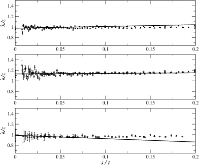
Figure 6: Top: effective critical exponent $\lambda/z$ calculated by power-law interpolation of $C(t,s)$ over the range $t\in[t_{\rm min};1500]$ versus $s/t_{\rm min}$ for the 4-state Potts model, the Baxter-Wu model and a multispin Ising model (from bottom to top). Bottom: fluctuation-dissipation ratio $X(t,s)$ versus $s/t$ for the same models (from left to right). The different symbols correspond to $s=10$ (circle), $s=20$ (square), $s=40$ (diamond), $s=80$ (triangle up) and $s=160$ (triangle left). The lattice size is $L=256$ for the 4-state Potts model and $L=258$ for the others.

6 Conclusions

We have addressed the question of universality for ageing ferromagnets, focusing on the study of the autocorrelation decay exponent $\lambda/z$ and the fluctuation-dissipation ratio $X_{\infty}$. It turns out that, apart from $X_{\infty}$ for the Ising model on triangular lattice, both $\lambda/z$ and $X_{\infty}$ do not depend on the particular lattice on which the models lives. This supports the idea of an extension of equilibrium universality classes to out-of-equilibrium processes. On the other hand, the Baxter-Wu model and a multispin Ising model, both belonging to the 4-state Potts model universality class at equilibrium, do not share the same exponent $\lambda/z$. Moreover, the 3-state Potts model and the Ashkin-Teller model, both belonging to the same universality class at equilibrium, have different exponents $\lambda/z$ but the same fluctuation-dissipation ratio $X_{\infty}$. This raises the question of the relevant quantities sufficient to characterise the universality class. Let us recall that we have not studied the influence of the dynamics itself on the universal quantities. It would be interesting for example to check whether the transition rates Eq. 17 and 18 lead to the same exponents and fluctuation-dissipation ratios or not.

References

References

- [1] Odor G, 2002 cond-mat/0205644 (to be published in Rev. Mod. Phys.).
- [2] Bray A J, 1994 Adv. Phys. 43, 357.
- [3] Hohenberg P C and Halperin B I (1977), Rev. Mod. Phys. 49, 435.
- [4] Fisher D S and Huse D, 1988 Phys. Rev. B 38, 373.
- [5] Huse D, 1989 Phys. Rev. B 40, 304.
- [6] Wang F-G and Hu C-K, 1997 Phys. Rev. E 56, 2310.
- [7] Nightingale M P and Blöte H W J, 2000 Phys. Rev. B 62, 1089.
- [8] Schuelke L and Zheng B, 1995 Phys. Lett. A 204 295.
- [9] Majumdar S N, Bray A J, Cornell S J and Sire C, 1996 Phys. Rev. Lett. 77, 3704.
- [10] Janssen H K, Schaub B and Schmittmann B, 1989 Z. Phys. B 73, 539.
- [11] Li Z B, Schülke L and Zheng B, 1995, Phys. Rev. Lett. 74, 3396.
- [12] Li Z B, Liu X W, Schülke L and Zheng B, 1997 Physica A 245, 485.
- [13] Arashiro E and Drugowich de Felício J R, 2003 Phys. Rev. E 67, 046123.
- [14] Simes C S and Drugowich de Felício J R, 2001 Mod. Phys. Lett. B 15, 487.
- [15] Cugliandolo L F and Kurchan K, 1994 J. Phys. A 27, 5749.
- [16] Chatelain C, 2003 J.Phys. A 36, 10739.
- [17] Calabrese P and Gambassi A, 2002 Phys. Rev. E 66, 066101.
- [18] Godrèche C and J-M. Luck J-M, 2000 J.Phys. A 33, 9141.
- [19] Mayer P, Berthier L, Garrahan J P and Sollich P (2003), Phys. Rev. E 68, 016116.
- [20] Calabrese P and Gambassi A, 2003 Phys. Rev. E 67, 036111.
- [21] Sastre F, Dornic Y and Chaté H, 2002 Phys. Rev. Lett. 91, 267205.
- [22] Henkel M and Schütz G M, 2004 J. Phys. A 37, 591.
- [23] Ising E, 1925 Zeits. f. Physik 31, 253.
- [24] Kramers H A and Wannier G H, 1941 Phys. Rev. 60, 252.
- [25] Kim D and Joseph R I, 1974 J. Phys. C 7, L167.
- [26] Potts R B, 1952 Proc. Camb. Philos. Soc. 48, 106.
- [27] Ashkin J and Teller E, 1943 Phys. Rev. 64, 178.
- [28] Fan C, 1972 Phys. Rev. B 6, 902.
- [29] Baxter R J and Wu F Y, 1973 Phys. Rev. Lett. 71, 1294.
- [30] Turban T, 1982 J. Physique 43, L259.
- [31] Glauber R J, 1963 J. Math. Phys 4, 294.
- [32] Ricci-Tersenghi F, 2003 Phys. Rev. E 68, 065104
- [33] Abriet S and Karevski D, 2003 cond-mat/0309342.
- [34] Godrèche C, Krzakala F and Ricci-Tersenghi F, 2004 J. Stat. Mech. : Theor. Exp. P04007
- [35] Grassberger P, 1995 Physica A 214, 547.
- [36] Okano K, Schülke L and Zheng B, 1997 Nucl. Phys. B 485, 727.