Controlling many-body effects in the midinfrared gain and THz absorption of quantum cascade laser structures

Abstract

A many-body theory based on nonequilibrium Green functions, in which transport and optics are treated on a microscopic quantum mechanical basis, is used to compute gain and absorption in the optical and THz regimes in quantum cascade laser structures. The relative importance of Coulomb interactions for different intersubband transitions depends strongly on the spatial overlap of the wavefunctions and the specific nonequilibrium populations within the subbands. The magnitude of the Coulomb effects can be controlled by changing the operation bias.

I Introduction

The quantum cascade laser (QCL) has evolved, since its first experimental realization FAI94a , into an important device for infrared applications. Recently, lasing in the THz regime has been demonstrated, thus opening further perspectives KOE02 . The operation of these semiconductor heterostructure devices is based on optical intersubband transitions within the conduction band, which are the focus of this work. The importance of many-body effects on interband transitions is a well established fact Zim . The intersubband case has also been studied both experimentally and theoretically Helm:99 and is a topic of current research Li:03 ; Ines:03 . Typically, idealised cases of isolated quantum wells with equilibrium distributions for the carriers are considered in a two subband scenario, to facilitate the computational challenges. Assuming that only one level is occupied, exchange and depolarisation effects were found to be very relevant for both gain and absorption NIKO97 . Recent work has demonstrated the importance of fully solving the integral equation for the optical susceptibility for quantum wells Li:03 ; Ines:03 ; Ning:02 ; Gumbs:95 ; Faleev:02 . While standard semiconductor lasers based on interband transitions can be modelled by equilibrium distributions for electrons and holes with different quasi-Fermi levels PER98 , this is not appropriate for QCLs where a full kinetic theory is necessary to correctly determine the nonequilibrium populations of the multiple level system.

The main issues of our paper are: (i) the question how these many-body effects are affected by the inherent nonequilibrium distribution in a QCL, where the interplay of a large number of different levels is crucial for the operation of the device; (ii) to what extent many-particle corrections can be modified in a given structure out of equilibrium and in a complex wavefunction scenario.

We show that a characteristic QCL design provides rather small overall Coulomb corrections to the gain transitions in the infrared, while significant level shifts occur in the THz absorption region. The latter depend strongly on the bias applied to the structure, which opens a possibility for a systematic variation of Coulomb effects in an experimental study of a complex nonequilibrium system. Here a wider variation of parameters is possible compared with previous experimental studies in quantum wells by either applying a bias Tsu:00 ; Luin:01 or optically pumping a laser Liu:00 .

Our findings thus give evidence of the need of our more advanced approach to model complex nonequilibrium studies. The study of simple structures in ref. NIKO97 would suggest similar strengths of Coulomb corrections in both gain and absorption regimes. Although those results are qualitatively correct for the cases previously studied, they can not be used for more complex structures of current interest, as demonstrated in our analysis, since the Coulomb matrix elements and occupation functions are extremely different for gain and absorption transitions. That large discrepancy is explained here for the first time to the best of our knowledge.

II Main Equations

Our calculations are based on the stationary state under operating conditions which is obtained by a self-consistent solution of the quantum kinetic equations LEE02a . Here scattering with phonons and impurities are included via the respective self-energies in the Dyson equations, and electron-electron interaction is treated in mean field approximation. The lattice temperature only enters via the phonon bath at 77 K, which is assumed to be in thermal equilibrium, neglecting hot phonon effects COM02 . For each subband, the nonequilibrium occupation functions, $f_{\nu}(k)$ are calculated from the diagonal terms in the carrier Green functions $G^{<}_{\nu\nu}({\bf k},\omega)$ which are expanded in terms of eigenstates $\phi_{\nu}(z)$ of the single particle Hamiltonian including the mean field. (These states will be referred to as levels in the following.) The calculated dephasing $2\Gamma_{\nu}$ is the FWHM of the spectral function, ${\Im}\{G^{\rm ret}_{\nu\nu}({\bf k=0},\omega)\}$ and $E_{\nu}({\bf 0})$ the corresponding location of the peak of the spectral function so that the electronic states are well defined quasi-particles, whose properties are evaluated on a microscopic basis. The optical absorption $\alpha$ at a given photon energy $\hbar\omega$ can be calculated from the imaginary part of the optical susceptibility,

$$\alpha(\omega)=\frac{4\pi\omega}{cn_{b}}{\Im}\{\chi(\omega)\},\;\;\chi(\omega)=2\sum_{\mu\neq\nu,\vec{k}}\,\wp_{\mu\nu}\,\chi_{\nu,\mu}(k,\omega).$$ (1)

Here $n_{b}$ denotes the background refractive index, $c$ is the speed of light, $\wp_{\nu\mu}$ is the transition dipole moment between the subbands $\nu$ and $\mu$, which are labelled $\nu=1,2,\ldots$ with increasing energy. In our calculation we select the 9 lowest subbands per period. The definition of a period (and thus the choice of level 1) is of course arbitrary in such structures and we must also take into account transitions between neighbouring periods. Numbering the levels in the next period to the left by 10–18, we consider all transitions $(1,\ldots 9)\leftrightarrow(1,\ldots 18)$ in the computations. We evaluate the susceptibility function, $\chi_{\nu\mu}(k,\omega)$, by the carriers’ Keldysh Green’s function, $G$, whose time evolution is described by a Dyson equation, with Coulomb interactions as well as other scattering mechanisms included in self-energies, $\Sigma$ PER98 . The general theory includes carrier-carrier scattering, diagonal and non-diagonal dephasing. In the numerical results presented here, we keep only the subband shift, depolarisation and exchange terms in the electron-electron interaction (Hartree-Fock). Similarly to the interband case, PER98 but with additional terms due to depolarisation as well as full consideration of a Hartree (mean field) term in the quasi-free particle term $E_{\nu}(\bf k)$, the resulting integral equation for the susceptibility function reads,

$$\left[\hbar\omega-e_{\nu\mu}({\bf k})+i\left(\Gamma_{\mu}+\Gamma_{\nu}\right)\right]\chi_{\nu\mu}({\bf k},\omega)+\left(f_{\nu}({\bf k})-f_{\mu}({\bf k})\right)\;2\;V\left({\nu\;\mu\;\mu\;\nu\atop 0}\right)\;\sum_{{\bf k}^{\prime}}\chi_{\nu\mu}({\bf k}^{\prime},\omega)\\ -\left(f_{\nu}({\bf k})-f_{\mu}({\bf k})\right)\;\sum_{{\bf k}^{\prime}\neq{\bf k}}\chi_{\nu\mu}({\bf k}^{\prime},\omega)\;V\left({\nu\;\nu\;\mu\;\mu\atop{\bf k}-{\bf k}^{\prime}}\right)=\wp_{\nu\mu}\left(f_{\nu}({\bf k})-f_{\mu}({\bf k})\right)\,.$$ (2)

Terms with more then two different indices vanish identically in the limit of isolated wells with infinite confinement barriers and remain small in the more complex structure studied here. The bare Coulomb interaction is given by

$$V\left({\mu\;\nu\;\lambda\;\beta\atop{\bf k}-{\bf k}^{\prime}}\right)=\int dz\,dz^{\prime}\,\phi^{\ast}_{\mu}(z)\phi_{\nu}(z)\frac{2\pi e^{2}\,\exp{\left(-|{\bf k}-{\bf k}^{\prime}||z-z^{\prime}|\right)}}{\epsilon_{0}A|{\bf k}-{\bf k}^{\prime}|}\,\phi^{\ast}_{\lambda}(z^{\prime})\phi_{\beta}(z^{\prime}),$$ (3)

where we have introduced the normalisation area $A$, and the background dielectric constant $\epsilon_{0}$. The explicit expressions actually programmed here are given in the Appendix.

$$\begin{split}e_{\nu\mu}({\bf k})=&E_{\nu}({\bf k})-E_{\mu}({\bf k})-\sum_{{\bf k}^{\prime}}f_{\nu}({\bf k}^{\prime})\;V\left({\nu\;\nu\;\nu\;\nu\atop{\bf k}-{\bf k}^{\prime}}\right)+\sum_{{\bf k}^{\prime}}f_{\mu}({\bf k}^{\prime})\;V\left({\mu\;\mu\;\mu\;\mu\atop{\bf k}-{\bf k}^{\prime}}\right)\\ &+\sum_{{\bf k}^{\prime}}[f_{\nu}({\bf k}^{\prime})-f_{\mu}({\bf k}^{\prime})]\;V\left({\nu\;\mu\;\mu\;\nu\atop{\bf k}-{\bf k}^{\prime}}\right)\,,\end{split}$$ (4)

is the energy difference between the levels renormalised by the exchange interaction, which we refer to as subband shift in the following. The second term on the left-hand side of Eq. (2) gives rise to the depolarisation shift, while the last term (exchange contribution) is analogous to the excitonic coupling term in interband transitions PER98 . The equations above reduce to those of Ref. CHU92 in the two-band limit at equilibrium. Note that by running over all subband indices $\nu\neq\mu$ in Eqs. (1,2), we do not apply the rotating wave approximation.

III Numerical Results and Discussion

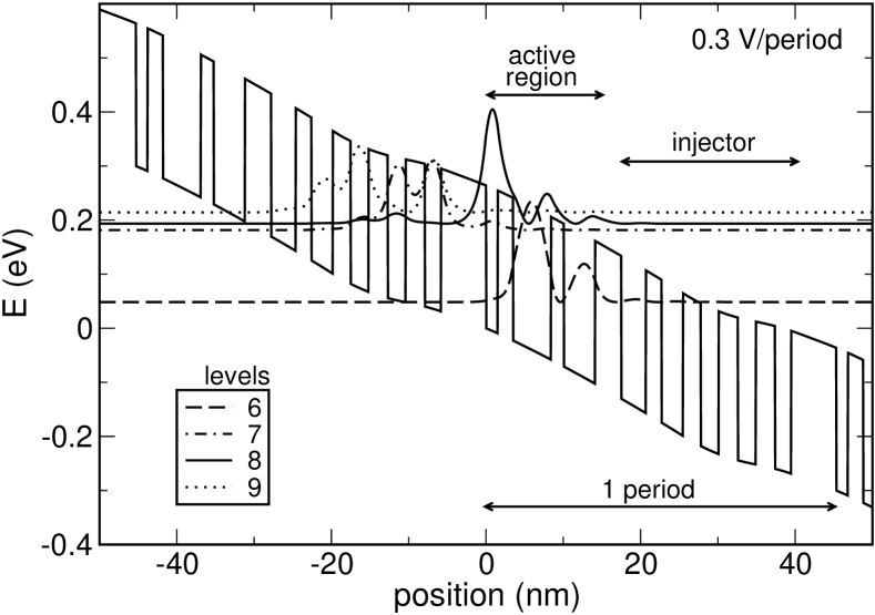
Figure 1: Section of the quantum cascade laser structure and a few relevant levels within a period, including mean field effects due to the ionised dopants in the structure, and for a bias V=0.3 V/period. Level 7 is an injector level. Levels 6 and 8 yield the main contribution for the midinfrared gain spectrum, while levels 7 and 9 are responsible for the main THz absorption feature.

For numerical applications of the theory, we choose the very successful prototype introduced by Sirtori et al. SIR98 , see Fig. 1. From a systematic study of doping dependence GIE03 it was found that the performance is best for a doping around $6.4\times 10^{11}/\textrm{cm}^{2}$ which is used throughout this work together with a lattice temperature of 77 K unless stated otherwise.

In Fig. 2 we compare the absorption spectra evaluated with and without Coulomb effects for different biases. We find that gain sets in around 0.2 V/period at energies $\hbar\omega\approx 130$ meV (infrared region) in good agreement with the experimental findings GIE03 . In addition there is a pronounced absorption around 30 meV (THz-region). While the Coulomb effects are hardly visible in the gain region, significant shifts of peak height and position occur in the THz absorption lines, in particular at low bias.

In the following we present a systematic study of the Coulomb terms in Eq. (2), which crucially depend on the Coulomb matrix elements and the occupation differences, which are displayed in Table 1 for the dominant transitions. A glance at the values $n_{\nu}-n_{\mu}$ [which roughly scale with $f_{\nu}({\bf k})-f_{\mu}({\bf k})$] shows that the structure is out of equilibrium, as necessary for laser operation. In order to quantify changes in Coulomb effects, we express the matrix element for the depolarisation term as $L^{dep}_{\nu\mu}=\frac{9\pi\epsilon_{0}A}{20e^{2}}\,V^{\nu\mu\mu\nu}_{0}$, so that it reduces to the well width in the limiting case of a quantum well with infinite confinement barriers for transitions between the two lowest subbands. This reflects the common knowledge that the depolarisation shift increases with well width, i.e. increasing spatial extension of the wave functions. For a QCL the scenario is much more involved, as the spatial overlap of the wave functions essentially contributes to the Coulomb effects as well. Similar quantities can also be defined for the exchange and subband shift, namely $L^{ex}_{\nu\mu}$, and $L^{bg}_{\nu\nu}$. Explicit expressions are derived in the Appendix and numerical values are given in Table 1. In contrast to $L^{dep}$, both $L^{ex}$, and $L^{bg}$ are inversely proportional to the corresponding Coulomb matrix elements. We can then expect that relatively large $L^{dep}$ and small $L^{ex}$ should correspond to large dipole moments, or in other words, to strong overlap between the wavefunctions of the levels involved in the transition. Only the wavefunction for level $\nu$ appears in $L^{bg}_{\nu\nu}$. Thus, its value remains within the same order of magnitude irrespective of the transition. Note that the significant difference between the values of $L^{dep},L^{ex}$, and $L^{bg}$ as well as for the different transitions further demonstrates that results from a simplified two-level system in a quantum well, where these lengths are identical by definition, cannot be easily generalised to more complex scenarios, like the real QCL structure discussed here.

In the THz region, $L^{dep}_{\nu\mu}$ and the dipole moment $\wp_{\nu\mu}$ tend to decrease with increasing bias, due to the changes in the wave function overlap. Furthermore the population decreases in the injector. This explains the general trend that the Coulomb effects become weaker with increasing bias. At 0.2 V/period, the concentration of the population in the lowest injector level 7 leads to a very strong absorption feature in the THz region although $L^{dep}_{\nu\mu}$ is smaller than at 0.12 V/period. In the infrared region, the larger bias increases the occupation of the subbands which are responsible for laser action. Furthermore both $L^{dep}_{\nu\mu}$ and $\wp_{\nu\mu}$ increase with bias as the injector levels leak into the active region. Nevertheless $L^{dep}_{\nu\mu}$ is much smaller than in the THz absorption region, and furthermore the compensation between the different many-particle effects (see below) in the dominating gain transitions leads to very small resulting shifts in Fig. 2. The contrast between the interesting Coulomb shifts in the low energy side and the almost vanishing shift in the high energy gain side is dramatic. This is the reason why gain calculations without Coulomb corrections LEE02a could explain experimental gain spectra in this structure reasonably well, but will fail in the absorption region. The main contributions to the absorption in the THz region are in fact transitions involving the two lowest injector levels at each bias. In other words, levels 6 and 7 for 0.12 V/period, levels 7 and 8 for 0.2 V/period and levels 7 and 9 for 0.3 V/period.

The interplay between the different Coulomb corrections in the THz region is analysed in more detail in Fig. 3. We select the dominant transitions for each bias to highlight the different contributions more clearly. The general tendency is that the exchange contribution imparts a red-shift while subband shift and depolarisation terms lead to blue-shifts. The depolarisation shift decreases with bias (in accordance with the discussion above), while the tendency of the exchange contribution and the subband shift is less clear. These two terms almost cancel each other, so that the blue-shift due to depolarisation dominates the behaviour. Because the subband shift slightly overcompensates the exchange contribution, the full Hartree-Fock curve exhibits a small additional blue-shift, in particular for 0.2 V/period.

Figure 4 shows details for the two dominating gain transitions at 0.3 V/period. We notice first that all many-particle effects reverse sign for gain transitions. This is due to the sign change in the occupation differences entering Eqs. (2,4) NIKO97 . Both transitions exhibit a red-shift due to all the Hartree-Fock corrections. The shift is stronger for the (6,7) transition although the depolarisation length is much smaller compared to the (6,8) transition, see Table 1. For gain transitions a significant part of the upper laser level is located in the injector, resulting in a weaker spatial overlap of the wave functions $\phi_{\mu}$ and $\phi_{\nu}$. Thus the Coulomb matrix elements entering exchange and depolarisation corrections (such as $L^{dep}_{\nu\mu}$) are reduced compared to the THz absorption within the injector region. In contrast Coulomb matrix elements of the type $V(\mu,\mu,\mu,\mu)$ enter the subband shift (4), which therefore dominates the behaviour in the gain region. Indeed, a lookup at Table 1 shows that $L^{dep}$ is small, $L^{ex}$ is large, consistently with the small dipole transition moment, while $L^{bg}$ is relatively small, leading to the scenario depicted in Fig. 4.

The spectra of typical QCLs are found to result from a delicate interplay of different transitions with strongly varying transition parameters. Standard approaches for idealised quantum wells cannot describe this situation, where the full nonequilibrium distribution obtained from quantum transport LEE02a , or possibly semi-classical Monte-Carlo IOT01a simulations, must be combined with the correct wavefunctions for a consistent description and understanding of the detailed spectra. Table 1 shows that $L^{dep}_{\nu\mu}$ and $\wp_{\nu\mu}$ can be easily modified within the same structure by changing the bias. This allows for a systematic experimental study of the magnitude of Coulomb effects as a function of transition parameters. Thus QCLs constitute promising structures to investigate the influence of Coulomb effects on intersubband transitions. A central issue of such experimental studies as well as future theoretical work will be the importance of higher order Coulomb corrections together with a more stringent treatment of screening compared to our Hartree-Fock approach. Recent work indicates that compensations between diagonal and nondiagonal terms Ines:03 may strongly reduce the importance of higher-order electron-electron scattering terms in simple model structures. This indicates that neglecting scattering in our Hartree-Fock approach may be a reasonable approximation, although this requires further detailed investigation.

Furthermore we illustrate the importance of many body effects as compared to the free carrier model as a function of both doping densities and temperatures. In order to keep our discussion as close as possible to experimental realizations, we chose densities and temperatures compatible with the samples described in Refs. SIR98 ; GIE03 .

Figure 5 shows the absorption spectra with and without Hartree-Fock Coulomb corrections for different doping densities. Our free carrier model includes the mean field of the ionised dopants and as the density increases, they shift the peak of the main absorption transition to the blue. The many-body effects impart a further intersubband blue shift and increase in oscillator strength of the main transitions. Although both the subband shift and overall oscillator strength increase with carrier density, the impact of the Coulomb corrections is similar for all densities and follows our detailed analysis of the N=6.4 $\times$ $10^{11}$/cm² case given above.

The density dependence study is complemented with Fig. 6 that depicts the evolution of gain (-absorption) spectra with density. Maximum gain is reached around N=4.6 $\times$ $10^{11}$/cm². The lower panels show that Coulomb corrections are larger for the larger density and the inset depicts the evolution of peak gain position with doping. Although the corrections are small it is interesting to note that Coulomb corrections lead to smaller increase in peak gain position on the high density, making the results slightly closer, qualitatively, to the experimental findings of Ref. GIE03 . However, Coulomb effects only are not enough to explain their results and a more detailed analysis is required.

We close our analysis with Fig. 7 where we show the influence of temperature on the calculated curves with (solid) and without (dot-dashed) many-body effects. The top and lower panels are respectively for phonon bath temperatures T=77 and 180 K. In both panels, the bias is V=0.2 V/period and the carrier density N= 6.4 $\times$ $10^{11}$/cm².

The rise in temperature increases the spectral broadening and promotes a redistribution of population difference, favouring the gain transitions As a consequence, the resulting subband shift is not so pronounced in the low energy side in comparison to T=77K. However, since different transitions have different Coulomb corrections, the inclusion of Coulomb effects at T=180 K affects the qualitative shape of the spectrum more strongly at higher temperatures. Structures that appear on the low energy side can not be seen with a free carrier model.

This manifests a further example of the complicated interplay between the different levels in the QCL structure, which is not present in simple two-level systems.

Another interesting remark is that, for larger dephasing, the counter-rotating terms, usually very small and ignored Li:03 , start to be relevant. The Coulomb shifts have opposite directions for counter rotating terms than for rotating wave contributions, and they should yield interesting effects in structures specifically constructed to study their relevance.

IV Summary

In summary, our nonequilibrium many-body theory yields a surprising contrast between the importance of Coulomb effects at the absorption and gain region in quantum cascade structures. While these effects are small in the gain region for the structure considered, strong features appear at THz absorption.

The many-body effects are influenced by both nonequilibrium occupation functions and Coulomb matrix elements, which depend on wavefunction overlap. Those two factors can be modified by means of an external bias which ultimately allows us to control the overall strength of Coulomb corrections in the structure.

Appendix A Interpolation Formula for Coulomb Matrix Elements

The Coulomb matrix elements in Eq. 3 can be difficult to evaluate numerically, and we give here tractable expressions for the relevant terms. In general, the Coulomb matrix elements are given by

$$V\left({\mu\;\nu\;\lambda\;\beta\atop q}\right) = V^{2d}_{q}\;F\left({\mu\;\nu\;\lambda\;\beta\atop q}\right),$$ (5)

$$F\left({\mu\;\nu\;\lambda\;\beta\atop q}\right) = \int dz\,dz^{\prime}\,\phi^{\ast}_{\mu}(z)\phi_{\nu}(z)\exp{\left(-q|z-z^{\prime}|\right)}\,\phi^{\ast}_{\lambda}(z^{\prime})\phi_{\beta}(z^{\prime}),$$

$$V^{2d}_{q}=\frac{2\pi e^{2}}{\epsilon_{0}Aq}.$$

As pointed out in the text, $V^{\nu\mu\mu\nu}_{0}$ matrix elements can be expressed exactly as a depolarisation length in the small wavenumber limit,

$$L^{dep}_{\nu\mu}=\frac{9\pi\epsilon_{0}A}{20e^{2}}\,V^{\nu\mu\mu\nu}_{0}.$$ (6)

The large wavenumber limit reads

$$V\left({\nu\;\mu\;\mu\;\nu\atop q\rightarrow\infty}\right) = V^{2d}_{q}\;\frac{1}{q\,b_{\mu\nu}},$$ (7)

$$\frac{1}{b_{\mu\nu}} = 2\int dz\,|\phi_{\mu}(z)|^{2}\,|\phi_{\nu}(z)|^{2}.$$

Inspection of the two extremes, suggests an interpolation formula for the depolarisation-like terms,

$$V\left({\nu\;\mu\;\mu\;\nu\atop q}\right) = V^{2d}_{q}\;\frac{q}{\frac{9\pi^{2}}{10L^{dep}_{\nu\mu}}+b_{\mu\nu}q^{2}}.$$ (8)

Similar considerations yield an analogous interpolation formula for the subband shift and exchange matrix elements,

$$V\left({\nu\;\nu\;\nu\;\nu\atop q}\right) = V^{2d}_{q}\;\frac{1}{1+\frac{L^{bg}_{\nu\nu}}{3}q},$$ (9)

$$V\left({\nu\;\nu\;\mu\;\mu\atop q}\right) = V^{2d}_{q}\;\frac{1}{1+\frac{L^{ex}_{\nu\mu}}{2}q},$$

where

$$L^{bg}_{\nu\nu} = \frac{3/2}{\int dz\,|\phi_{\nu}(z)|^{4}},$$ (10)

$$L^{ex}_{\nu\mu} = \frac{1}{\int dz\,|\phi_{\mu}(z)|^{2}\,|\phi_{\nu}(z)|^{2}}.$$

The lengths, $L^{dep}_{\nu\mu}$, $L^{ex}_{\nu\mu}$, $L^{bg}_{\nu\nu}$ have been defined so that they reduce to the quantum well width if the wavefunctions used are the eigenstates of an infinite potential well.

Bias	($\nu$,$\mu$)	$L^{dep}_{\nu\mu}$	$\wp_{\nu\mu}$	$n_{\nu}-n_{\mu}$	$E_{\mu}-E_{\nu}$	$\Gamma_{\nu\mu}$	$L^{ex}_{\nu\mu}$	$L^{bg}_{\nu\nu}$	$L^{bg}_{\mu\mu}$
0.12	(6,7)	25.8	4.99	2.44	13.3	5.3	14.9	25.0	30.3
0.12	(7,10)	20.5	4.56	1.33	24.2	9.1	16.5	30.3	27.6
0.2	(7,8)	19.3	4.23	3.19	23.9	3.1	17.2	20.4	27.4
0.2	(8,10)	18.5	3.96	0.87	25.3	9.0	14.0	27.4	31.6
0.2	(4,9)	3.2	1.38	-0.36	129.5	23.6	33.0	21.1	13.9
0.3	(7,9)	12.3	2.50	2.08	32.8	6.2	12.8	18.5	22.2
0.3	(8,11)	11.7	2.92	1.07	73.9	14.4	12.2	14.2	33.7
0.3	(6,7)	0.28	0.43	-2.60	129.5	15.5	371.4	13.0	18.5
0.3	(6,8)	4.5	1.68	-1.08	139.2	19.3	20.6	13.0	14.2

Table 1: Absorption/gain transition parameters. The first column is in Volts/period. ($\nu$,$\mu$) denotes the lower and higher subbands in a transition, $n_{\nu}-n_{\mu}$ is the difference in subband population in units $10^{11}/\mathrm{cm}^{2}$. $L^{dep}_{\nu\mu}$ $L^{ex}_{\nu\mu}$ , $L^{bg}_{\nu\nu}$, and $L^{bg}_{\mu\mu}$ are in nm and $\wp_{\nu\mu}$ in $e\times$nm. $E_{\mu}-E_{\nu}$ is the energy difference in meV at k=0 of Eq. (4), i.e. including the static mean field corrections, but no further Coulomb effects. $\Gamma_{\nu\mu}$ = $\Gamma_{\nu}+\Gamma_{\mu}$ is the dephasing in meV.

Figure 2: Influence of bias on absorption/gain spectra. From top to bottom the bias is V=0.3, 0.2 and 0.12 V/period. In all panels, the dot-dashed lines are for free carriers, while the solid curves have full Hartree-Fock Coulomb corrections.

Figure 3: Details of THz absorption including mean field effects in the dominant transition of each bias. From bottom to top, the bias is V= 0.12, 0.2 and 0.3 V/period, and the corresponding transitions are between levels (6,7), (7,8) and (7,9) as discussed in the text. In all panels, the solid, dotted, short-dashed, long-dashed and dot-dashed curves are respectively for Full Hartree-Fock, sub-band shift only, depolarisation only, exchange only, and free carriers.

Figure 4: Details of the main transitions that contribute to the gain spectra including mean field effects for a bias V= 0.3 V/period. The lower and top panels are respectively for (6,8) and (6,7) transitions. In both panels, the solid, dotted, shot-dashed, long-dashed and dot-dashed curves are respectively for Full Hartree-Fock, sub-band shift only, depolarisation only, exchange only, and free carriers.

Figure 5: Comparison of absorption spectra with (solid) and without (dot-dashed) Hartree-Fock Coulomb corrections. In all panels the bias is V=0.2 V/period. The carrier densities are given respectively by N=3.5, 4.6, 5.25, and 7 $\times$ $10^{11}$/cm².

Figure 6: Gain spectra as a function of doping. All curves in the top panel have full Hartree-Fock corrections. The solid, dotted, long-dashed and dot-dashed curves correspond, respectively to N=3.5, 4.6, 6.4 and 7 $\times$ $10^{11}$ /cm². The inset depicts the spectral position of peak gain (in meV) as a function of doping in $10^{11}$ /cm². The open squares are for full Hartree-Fock while the circles are for free carriers. The symbols are connected by solid and dot-dashed lines respectively to guide the eye. In the central and bottom panels, the dopings are, respectively, N=3.5 and 7 $\times$ $10^{11}$ /cm². The solid and dot-dashed curves are respectively for full Hartree-Fock and free-carrier calculations.

Figure 7: Comparison of absorption spectra with (solid) and without (dot-dashed) Hartree-Fock Coulomb corrections for a bias of 0.2 V/period . The top and lower panels are respectively for phonon bath temperatures T=77 and 180 K.

References

- (1) Present Address: Department of Physics, University of Lund, Box 118, 22100 Lund, Sweden.
- (2) J. Faist, F. Capasso, D. L. Sivco, C. Sirtori, A. L. Hutchinson, and A. Y. Cho ,Science 264, 553 (1994).
- (3) R. Kohler, A. Tredicucci, F. Beltram, H. E. Beere, E. H. Linfield, A. G. Davies, D. A. Ritchie, R. C. Iotti and F. Rossi, Nature, 417, 156 (2002).
- (4) R. Zimmermann, Many Particle Theory of Highly Excited Semiconductors (Teubner, Leipzig, 1987).
- (5) M. Helm, in Intersubband Transitions in Quantum Wells: Physics and Device Applications, edited by E. R. Weber and R. K. Willardson (Academic Press), 62, 1 (1999).
- (6) J. Li and C. -Z. Ning, Phys. Rev. Lett. 91, 097401 (2003).
- (7) I. Waldmüller, M. Woerner, Jens Förstner, and A. Knorr Phys. stat. sol. b 238, 474 (2003).
- (8) D. E. Nikonov, A. Imamoglu, L. V. Butov, and H. Schmidt, Phys. Rev. Lett. 79 4633 (1997).
- (9) J. Li, C. Z. Ning, D. C. Larraber, G. A. Khodaparast, J. Kono, K. Ueda, Y. Nakajima, S. Sasa, and M. Inoue, in Progress in Semiconductors II edited by B.D. Weaver, (Proceedings of the MRS) bf 744, 571 (2003).
- (10) G. Gumbs, D. Huang, and J.P. Loehr, Phys. Rev. B51, 4321 (1995).
- (11) S.V. Faleev, and M.I. Stockman, Phys. Rev. B 66, 085318 (2002).
- (12) M. F. Pereira, Jr. and K. Henneberger, Phys. Rev. B 58, 2064 (1998).
- (13) S. Tsujino, M. Rüfenacht, H. Nakajima, T. Noda,C. Metzner, and H. Sakaki, Phys. Rev. B 62, 1560 (2000).
- (14) S. Luin, V. Pellegrini, F. Beltram, X. Marcadet, and C. Sirtori, Phys. Rev. B 64, 041306 (2001).
- (15) H. C. Liu and A. J. Spring Thorpe, Phys. Rev. B 61, 15629 (2000).
- (16) C. Sirtori, P. Kruck, S. Barbieri, P. Collot, J. Nagle, M. Beck, J. Faist, and U. Oesterle, Appl. Phys. Lett. 73, 3486 (1998).
- (17) M. Giehler, R. Hey, H. Kostial, S. Cronenberg, L. Schrottke, and H. T. Grahn, Appl. Phys. Lett. 82, 671 (2003).
- (18) S. C. Lee and A. Wacker, Phys. Rev. B 66, 245314 (2002).
- (19) F. Compagnone, A. Di Carlo, and P. Lugli, Appl. Phys. Lett. 80, 920 (2002).
- (20) S. L. Chuang, M. S. C. Luo, S. Schmitt-Rink and A. Pinczuk, Phys. Rev. B 46, 1897 (1992).
- (21) R. C. Iotti and F. Rossi, Phys. Rev. Lett. 87, 146603 (2001).