Semiclassical dynamics of domain walls in the one-dimensional Ising ferromagnet in a transverse field

Abstract

We investigate analytically and numerically the dynamics of domain walls in a spin chain with ferromagnetic Ising interaction and subject to an external magnetic field perpendicular to the easy magnetization axis (transverse field Ising model). The analytical results obtained within the continuum approximation and numerical simulations performed for discrete classical model are used to analyze the quantum properties of domain walls using the semiclassical approximation. We show that the domain wall spectrum shows a band structure consisting of 2$S$ non-intersecting zones.

I Introduction

Nonlinear topologically nontrivial excitations, or solitons, are known to exist in lower-dimensional magnetic systems. There is both theoretical and experimental evidence of solitons and in some cases soliton effects dominate the thermodynamic behavior of one-dimensional (1D) magnets (spin chains). Soliton effects possibly emerged first when absence of long range order in lower-dimensional magnets was proved: From simple entropy arguments it has been shown that long range magnetic order is not possible in one-dimensional magnets at nonzero temperature and it became clear later that kink-type solitons, which in fact are magnetic domain walls (DW), must be considered as elementary excitations at nonzero temperature in one-dimensional magnets, for reviews see mikeska ; sowsci . Whereas solitons in one-dimensional magnets have not been directly observed, dynamic soliton effects such as soliton motion and the soliton-magnon interaction result in soliton contributions to the dynamic response functions, which can be studied experimentally. For example, solitons contribute to the specific heat and to the linewidth of electron spin resonance and the translational motion of kinks leads to the so-called soliton central peak, which can be detected through neutron scattering experiments.mikeska ; sowsci

In most approaches solitons have been considered using classical continuum models, such as the Landau-Lifshitz equations or the sine Gordon equation, see Refs. mikeska, ; sowsci, ; phys.rep, . On the other hand, in order to describe a material such as CsCoCl₃ the XXZ-model with spin $S=1/2$ has to be used, and solitons occur as quantum objects.villain ; mikeska+ Even for the material CsNiF₃, the well-known standard example for classical solitons in 1D magnets, quantum effects due to its spin $S=1$ are essential.mikeska Although a detailed analysis concentrated on classical models, considerable achievements in the field of quantum solitons were obtained rather early: We note, first of all, that the first nonlinear excitations (spin complexes) were investigated by Bethe in the isotropic one-dimensional ferromagnet as long ago as 1931, essentially in parallel with the prediction of magnons.bethe Currently it is established that the more general XYZ-model with spin $S=1/2$ is exactly integrable, and the quantum nonlinear excitations (spin complexes) are known from the solution of this model.baxter

At first sight quantum and classical solitons constitute essentially different objects. The main property of classical solitons (or more precisely: solitary waves) is localization, while a quantum soliton is characterized by a definite value of the quasi-momentum $P$ and in virtue of this it is spatially delocalized. However, this contradiction is removed if one investigates the spin deviation localization in the coordinate system with the origin moving with the group velocity of the soliton.phys.rep The comparison of classical and quantum solitonsphys.rep reveals a striking feature of the XYZ-model: the dispersion law (the dependence of energy $E$ on the momentum $P$) of a spin complex in this model with spin $S=1/2$ exactly coincides with the corresponding dependence found for the soliton in the classical Landau-Lifshitz equations. It is evident that such an exact correspondence cannot be a general rule; probably it is associated with the exact integrability of both models. On the other hand, it has become clear that if one compares the characteristics which are relevant for both quantum and classical approaches, first of all the dispersion law $E=E(P)$, then there are no fundamental distinctions between quantum and classical solitons. Renewed interest in the problem of quantum properties of domain walls was stimulated due to the study of quantum tunneling DW chirality effects,ivkol ; br-loss ; TakagiTat96 ; TakagiShib00 ; Freire and also by the prediction of new effects of destructive interference in kink tunneling between neighboring crystal lattice sitesbr-loss and Bloch oscillations of the solitons.KirLoss98

The structure and the properties of solitons in the one-dimensional Ising model in the presence of a transverse magnetic field have been studied some time ago.mik-miyash It has been demonstrated in the semiclassical limit of large spin values $S\gg 1$ how classical localization correlates with quantum delocalization. Within the framework of the quantum approach the emergence of a band structure has been revealed. However, the quantum kink dispersion law found in this work has not been compared with the classical one. In Ref. mik-miyash, only static solutions of the classical problem have been used, and the comparison of the quantum kink dispersion law with those obtained within the semiclassical quantization model has not been made.

In this article we investigate analytically and numerically the dynamics of domain walls in a spin chain with ferromagnetic Ising interaction and subject to a magnetic field perpendicular to the easy magnetization axis (transverse field Ising model). Analytical results obtained within the continuum approximation and numerical simulations performed for the discrete classical model are used for the analysis of the semiclassical dynamics of domain walls including an account of the lattice pinning potential. We show that the spectrum of the DW in the classical continuum approximation is characterized by a periodic dependence of the kink energy on its momentum. This produces a number of non-trivial features for the DW motion in the presence of the pinning potential. The quantum properties of the domain wall are discussed on the basis of the semiclassical approximation. For the semiclassical dynamics the role of lattice pinning effects in the formation of the band structure of the domain wall spectrum is investigated. The presence of the periodic character of the DW dispersion law with lattice pinning taken into account results in a band structure for $E(P)$ with $2S$ non-intersecting branches.

The outline of this article is as follows. In Sec. II we formulate the discrete classical model and study the DW properties within this model. The main results of this section are the introduction of the DW coordinate, $X$, and the calculation of the pinning potential for the DW, $U(X)$. This is then used for the analysis of both the classical dynamics of the DW and its semiclassical quantization. In Sec. III the complementary continuum approach is used to investigate the motion of the DW with finite velocity. The DW linear momentum $P$ and the dispersion law of the DW, $E=E(P)$, are calculated, and $E(P)$ is found to be a periodic function of the momentum. The results for $U(X)$ and $E(P)$ are employed in the next two sections to describe the dynamics of the DW in the framework of the method of collective variables, assuming that the DW is an effective quasiparticle with kinetic energy $E(P)$, moving in the potential $U(X)$: In Sec. IV the specifics of forced DW motion as well as the detailed features of the band spectrum of the DW in the case of the weak potential $U(X)$ are discussed. The peculiarities of the dynamics of the DW in a finite potential associated with the periodic character of $E(P)$ are considered in Sec. V. Here it becomes clear that finite motion is typical for states which are either close to the minimum or close to the maximum of the potential $U(X)$. In Sec. VI we consider the quantum tunneling transitions between these states, corresponding to an adjacent unit cell. In this section the general character of the DW dispersion law including the effects of lattice pinning is discussed. Sec. VII gives our concluding remarks.

II The discrete model and a domain wall structure.

We start from the Hamiltonian describing a spin chain with Ising-type exchange interaction in a magnetic field $\vec{H}$ directed perpendicularly to the easy axis of a magnet. Spins $\vec{S}_{n}$ are located at points $na$ of a chain (distance $a$, $n$ integer),

$$\widehat{H}=-J\sum_{n}S_{n}^{z}S_{n+1}^{z}-g\mu_{B}H\sum_{n}S_{n}^{x}.$$ (1)

$J$ is the exchange integral, $g$ the gyromagnetic ratio and $\mu_{B}$ the Bohr magneton. The dimensionless field $h=g\mu_{B}H/2JS$ will be used in the following (the notation $2h=\gamma$ was used in Ref. mik-miyash ) This model is usually called transverse field Ising model.

For classical spins the ground state of the model at $h<1$ ($g\mu_{B}H<2JS$) is doubly degenerated with

$$S_{x}=S\sin\theta_{0},\ S_{z}=\pm S\cos\theta_{0},\ \sin\theta_{0}=h.$$ (2)

We begin to describe the semiclassical motion of the DW within the discrete spin model by studying the solutions for moving DW’s in the discrete classical model. We notice that the exchange part for the model of Eq. (1) is the simplest particular case of the so-called XYZ-model with three independent parameters $J_{1}\neq J_{2}\neq J_{3}$

$$\widehat{H}_{XYZ}=-\sum(J_{1}S_{n}^{x}S_{n+1}^{x}+J_{2}S_{n}^{y}S_{n+1}^{y}+J_{3}S_{n}^{z}S_{n+1}^{z}).$$

For an isotropic FM we have $J_{1}=J_{2}=J_{3}$ and DW’s strictly are absent (however, ’pulse solitons’ may exist) For the XXZ-model $(J_{1}=J_{2}<J_{3})$ in the absence of the magnetic field the exact static solution for the discrete model with classical spins has been constructed by GochevGochev . As far as we know this discrete problem has not yet been solved for $H\neq 0$ or for the more general classical XYZ-model even for $H=0$. The solution found by Gochev for the XXZ-model reads $S_{n}^{z}=S\tanh[\kappa(n-n_{0})]$, with $\kappa=\ln[(J_{3}+\sqrt{J_{3}^{2}-J_{1}^{2}})/J_{1}]$, where $1/\kappa$ measures the domain wall thickness. In the Ising limit the DW thickness goes to zero, $1/\kappa\rightarrow 0$ at $J_{1}\rightarrow 0$. We emphasize that the value of $n$ which describes the DW position in this solution (taken as $n=n_{0}$ above) is an arbitrary (not necessarily integer) number. Thus the model with $H=0$ has the nontrivial property that the energy of the DW does not depend on its center position for arbitrarily large anisotropy. It is not clear, whether this property is valid for the same Hamiltonian in the quantum case.

For the Ising model we easily understand the above result since at $H=0$ the DW is described by the following solution: $S_{n}^{z}=-S$ at $n<n_{0}$, $S_{n}^{z}=+S$ at $n>n_{0}$, however $S_{n}^{z}$ at $n=n_{0}$ may have arbitrary values. If $S_{n_{0}}^{z}=0$ the DW is localized on the spin with $n=n_{0}$; on the other hand, for $S_{n}^{z}=-S$ or $S_{n}^{z}=+S$ at $n=n_{0}$ the DW localized in the center of the bond which connects the spin at $n=n_{0}$ with spins at $n=n_{0}+1$ or $n=n_{0}-1$, correspondingly. For $H=0$ the energies of DW’s centered on the spin (central spin (CS) DW) or on the bond (central bond (CB) DW) coincide. For all intermediate cases $S_{n}^{z}\neq 0,\ \pm 1$ at $n=n_{0}$ it is natural to postulate that the DW is localized on a point $X$, which does not coincide with a site or the bond center and to describe the DW dynamics in terms of its coordinate $X$ treated as a collective variable. Let us introduce $X$ in the following way: we choose some lattice site and define the DW located on this site to have the coordinate $X=0$. Let us then find the $z$-projection $\mathcal{S}_{tot}^{z\ (0)}$ of the total spin $\mathcal{S}_{tot}^{z}$ of the DW localized on that site. It is then natural to determine the coordinate of any DW via the value of the total $z$-projection of the spin $\mathcal{S}_{tot}^{z}$, associated with this DW from the expression $X=a(\mathcal{S}_{tot}^{z}-\mathcal{S}_{tot}^{z\ (0)})/2S$. In order to account appropriately for possible divergencies in infinite chains the difference $\mathcal{S}_{tot}^{z}-\mathcal{S}_{tot}^{z\ (0)}$ is calculated as $\sum_{n=-\infty}^{n=\infty}[S^{z}_{n}(X)-S_{n}^{z}(X=0)]$ (here $S_{n}^{z}(X)$ and $S_{n}^{z}(X=0)$ are the $z-$ projection of spins on site $n$ for the DW with the coordinate $X$ and the DW with $X=0$ resp.). Then, for the DW in the model of Eq. (1) with $H\neq 0$ the complete definition reads

$$X=\frac{a}{2S\cos\theta_{0}}\sum_{n=-\infty}^{n=\infty}[S^{z}_{n}(X)-S_{n}^{z}(X=0)].$$ (3)

For zero field the DW energy $E$ does not depend on the coordinate $X$. At $H\neq 0$, as shown in Ref. mik-miyash, , a dependence of the DW energy on its coordinate emerges, pointing to the presence of a lattice pinning potential $U=U(X)$. The pinning potential $U(X)$ has its minimum value for $X=na$, i.e. for the CS DW, and its maximum value for $X=(a/2)(2n+1)$, i.e. for the CB DW.mik-miyash In order to investigate the nonstationary dynamics of the DW we will treat $U(X)$ as a potential energy. The analysis of the related kinetic energy will be discussed in the next section.

When the DW is moving in a discrete chain it is natural to use the periodic potential $U(X),\ U(X+a)=U(X)$. The form of the potential can be chosen as in br-loss ,

$$U(x)=U_{0}\sin^{2}(\pi X/a),$$ (4)

where $U_{0}$ characterizes the intensity of pinning caused by discreteness. With the choice of Eq. (4) for the potential, the value of $U_{0}$ can be found as the energy difference between the static central spin and central bond DW’s.mik-miyash In order to calculate $E_{CS}$ and E_CB we need in the solution of the corresponding classical discrete problem, which is known for small magnetic field only.mik-miyash Moreover, for our purpose we need to know not only the energy difference $E_{CS}-E_{CB}$, but the full dependence $U(X)$ in order to verify the dependence of Eq. (4).

To reveal $U(X)$ we have carried out a numerical analysis of the model of Eq. (1) in accordance with the definition Eq. (3) for the coordinate $X$. We have searched the conditional minimum of the energy as given by Eq. (1) for a finite spin chain at a fixed value of $\mathcal{S}_{tot}^{z}$. To solve this problem, the simplex type method with non-linear constraints was chosen as the method of minimization. This method is based on the steepest descent routine applied to functions of a large number of variables, and it is able to find the conditional minimum for a given function with fixing a small number of combinations to given values. The method exhibits a fast convergence when a spin distribution with only one domain wall placed near the point of inflection is used as starting condition. For our problem, the angular coordinates of each spin were chosen as variables, and the minimum of the energy was found with fixing the value of $\mathcal{S}_{tot}^{z}$. The DW was created by fixing the direction of two spins on the ends of the chain corresponding to Eq. (2). The chain length $N$ varied from 20 to 100, and for the the case of interest, $H\leq JS$, the result was independent of the chain length for $N\geq 30$. The value of $U_{0}$ in Eq. (4) was determined from the difference $E_{CS}-E_{CB}$; the behaviour of this quantity is shown in Fig. 1.

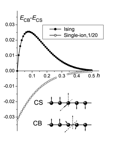
Figure 1: The difference of the energies (in units of $JS^{2}$) for CB and CS domain walls (shown schematically at the bottom of the figure) vs. magnetic field. The corresponding dependence for the model with single-ion anisotropy, normalized by 20, is also given for comparison (open circles).

Figure 2: Shape of the domain wall pinning potential $U(X)$ (in units of $JS^{2}$) for the dimensionless magnetic field $h=0.05$. Symbols denote the numerical data. The empirical dependence $0.024\sin^{2}(\pi x/2a)$, and a fit for a more general dependence with $U_{0}=0.024,\ U_{1}=-0.00255$ are shown as dashed and full lines, respectively.

The analysis shown in Fig. 2 demonstrates that in the case of interest to us, $h\ll 1$, $U(X)$ is fairly well described by Eq. (4). If we consider a more general dependence, allowing for one more Fourier component,

$$U(x)=U_{0}\sin^{2}(\pi X/a)+U_{1}\sin^{2}(2\pi X/a),$$ (5)

the dependence of $U(X)$ is reproduced with a deviation of less than $0.1\%$. However, as the correction related to $U_{1}$ is small, we will use in the following mainly the simplest expression, Eq. (4).

Note, as $U_{0}\rightarrow 0$ for $h\rightarrow 0$, and for $h\rightarrow 1$ the transverse field Ising model is characterized by a rather small pinning potential. For comparison, in Fig. 1 the corresponding dependence is presented for a ferromagnet with an isotropic Heisenberg interaction and a single ion anisotropy of the form $W_{a}=-\sum_{n}K(S_{n}^{z})^{2}$, which has the same amplitude as Eq. (4) at $K=J$. For this model $U_{0}$ has a maximum at $H=0$; the typical values of $U_{0}$ are approximately 20 times higher than for the transverse field Ising model. Furthermore, the quantity $U_{0}$ has opposite sign, i.e., in contrast to the transverse field Ising model one has $E_{CB}<E_{CS}$.

III Domain wall dynamics in continuum approximation.

Most of the results for the dynamics of domain walls or kink-type solitons in magnets have been obtained in the continuum approach, replacing $\vec{S}_{n}(t)$ by the smooth variable spin density $\vec{S}(x,t)$, where $x$ is the coordinate along the chain. Within this approach the dynamics of the vector field $\vec{S}(x,t)$ is described by the well known Landau-Lifshitz equation without dissipation LL (see also phys.rep ; sowsci )

$$\frac{\partial\vec{S}}{\partial t}=\frac{a}{\hbar}\left(\vec{S}\times\frac{\delta W\{\vec{S}\}}{\delta\vec{S}}\right).$$ (6)

Here $W\{\vec{S}(x,t)\}$ is the ferromagnetic energy as functional of the spin density. For our model, the transverse field Ising chain, $W\{\vec{S}(x,t)\}$ corresponds to the Hamiltonian of Eq. (1) and is written as: mik-miyash

$$W\{\vec{S}\}=\int\frac{dx}{a}\left\{J\frac{a^{2}}{2}\left(\frac{\partial S_{z}}{\partial x}\right)^{2}-JS_{z}^{2}-g\mu_{B}HS_{x}\right\}.$$ (7)

Using the continuum approach allows us to find a solution, which describes a DW moving with a given velocity $V$. On the other hand, the discreteness effects are evidently lost going from Eq. (1) to Eq. (7).

We use the relation $\vec{S}^{2}=S^{2}=\text{const}$ to write $\vec{S}=S\>\vec{m}(x,t)$ i.e. to express the spin through the unit vector field $\vec{m}(x,t)$. Its direction is determined by two independent variables, we will use the angular variables $\theta$ and $\varphi$,

$$m_{z}=\cos\theta,\;m_{x}=\sin\theta\cos\varphi,\;m_{y}=\sin\theta\sin\varphi.$$

In terms of these variables the Landau-Lifshitz Eq. (6) reads

$$\frac{\hbar S}{a}\sin\theta\frac{\partial\theta}{\partial t} = \frac{\delta W}{\delta\varphi},$$

$$\frac{\hbar S}{a}\sin\theta\frac{\partial\varphi}{\partial t} = -\frac{\delta W}{\delta\theta},$$ (8)

where $W\{\theta,\varphi\}$ is the ferromagnetic energy written as a functional of $\theta$ and $\varphi$. These equations can be considered as classical Hamiltonian equations for the canonically conjugate variables $\cos\theta$ (momentum) and $\varphi$ (coordinate), with Hamilton function $W$.

Kink solitons in such a continuum approach have been described for a number of magnetic chain models. These include the Heisenberg chain with two single ion anisotropies Sklyanin79 ; Mikeska80 ; EtrichMi83 , the Ising chain with transverse exchange breaking the $xy-$symmetry ElstnerMi89 and the $xy-$like Heisenberg chain with an external symmetry breaking field. EtrichMi88 ; EtrichMiMaThWe85 The qualitative results for kink solitons with permanent shape are analogous in all these models: The dispersion relation, energy vs. velocity, has two branches and one distinguishes between the lower energy domain wall (LDW) and the upper energy domain wall (UDW). The energies of these two solutions merge at the maximum possible velocity $V=V_{c}$. A more natural formulation results when the momentum is introduced instead of the velocity: then the dispersion relation becomes single valued and periodic with the magnetic unit cell.Haldane86 In particular the dispersion relations can be given explicitly for the Heisenberg chain with two single ion anisotropies. Sklyanin79 ; Mikeska80

Eqs. (6) or (III) are usually considered as purely classical equations. To discuss their applicability to the quantum regime one may use the quantum-field approach based on the spin coherent states formalism.fradkin Then the quantum phase (Berry phase) appears, leading to qualitative effects such as the suppression of quantum fluctuations for antiferromagnetic chains affleck and small magnetic particles with half-odd-integer total spin.quant-interf In this approach the spin state on every site $n$ is determined by the spin coherent state $|\vec{m}\rangle$, for which $\vec{S}\,|\vec{m}\rangle=S\,\vec{m}\,|\vec{m}\rangle$. Here $\vec{m}$, as before, is a unit vector, $\vec{m}^{2}=1$. In this approach, the dynamics of the mean value of spin $\vec{S}=S\vec{m}$ is described by a Lagrangian which can be written in the form

$$\mathcal{L}\{\vec{S}\}=\hbar S\int\frac{dx}{a}\vec{A}\dot{\vec{S}}-W\{\vec{S}\},$$ (9)

where

$$\vec{A}(\vec{S})=\frac{\vec{n}\times\vec{S}}{S(\vec{S}\vec{n}+S)}.$$ (10)

$\vec{n}$ is a unit vector with arbitrary direction, denoting the quantization axis for coherent states. It is important that $\vec{A}$ has the form of the vector potential of a magnetic monopole field in the full space $\{\vec{S}\}$ (not subject to the constraint $\vec{S}^{2}=\text{const}$).

The vector potential has a singularity (Dirac string) for $\vec{S}\,\vec{n}=-S$, i.e., on a half-line in space $\{\vec{S}\}$. Usually, the ”north pole” gauge with $\bm{n}=\bm{e}_{z}$ is used, then the quantity $\vec{A}(\vec{S})\,\dot{\vec{S}}$ acquires the familiar form

$$\vec{A}\dot{\vec{S}}=(1-\cos\theta)(\partial\varphi/\partial t).$$ (11)

In the saddle point approximation for the Lagrangians Eq. (9) or (11) one recovers the classical Landau-Lifshitz equations in the form of Eq. (6) or (III) for the mean value of spin $\vec{S}$. The potential $\vec{A}$ of the monopole field permits gauge transformations (in particular, the change of the direction of the spin quantization axis $\vec{n}$ and, hence, the positions of singularities). These do not change the equations of motion, but make a contribution to the Lagrangian in the form of a total time derivative of some function of spin. This may in principle be significant for the calculation of the DW momentum. Naturally, the classical equations are not affected by the gauge transform. On the other hand, the term with $\partial\varphi/\partial t$ in Eq. (11) is of crucial importance for the quantum dynamics of domain walls in spin chains with half-odd integer spins.br-loss For example, this term is responsible for the destructive interference of paths for DW tunneling from one minimum of the crystal potential to an adjacent one.br-loss

In order to construct a solution corresponding to a DW moving with velocity $V$, we have to write down the Landau-Lifshitz equations in angular variables, and to restrict ourselves to traveling wave-type solutions, $\theta=\theta(\xi),\ \varphi=\varphi(\xi),\ \xi=x-Vt$, with the natural boundary conditions, $S^{x}\rightarrow S\sin\theta_{0}$ at $\xi\rightarrow\pm\infty$, and

$$S^{z}\rightarrow\sigma S\cos\theta_{0},\ S^{z}\rightarrow-\sigma S\cos\theta_{0}$$

at $\xi\rightarrow\infty$ or $\xi\rightarrow-\infty$, respectively. Here $\sigma=\pm 1$ is $\pi_{0}$, the topological charge of the DW and $\cos\theta_{0}$ characterizes the ground state, see Eq. (2). Then, using Eq. (7), the equations for $\partial\theta/\partial t=-V\theta^{\prime}$ acquire the simple form $v\,\theta^{\prime}=-2h\sin\varphi$. Here and below the prime denotes differentiation with respect to $\xi$, and we have introduced the dimensionless variable

$$v=V/V_{0},\ V_{0}=aJS/\hbar$$

and put $a=1$ in all intermediate equations. We will restore the dimensional parameters in final results only.

The set of Eqs. (III) with the traveling wave ansatz has one integral of motion, which after taking boundary conditions into account can be written as

$$\frac{1}{2}[(\cos\theta)^{\prime}]^{2}-\sin^{2}\theta+2h\sin\theta\cos\varphi=h^{2}=\text{const}.$$ (12)

Using the simple relation between $\theta^{\prime}$ and $\sin\varphi$, this can be rewritten in the variable $\theta$ only. Finally we arrive at the simple differential equation for $\theta$,

$$(\cos\theta)^{\prime}=\sigma_{1}\sqrt{2\sin^{2}\theta-v^{2}}+\sigma_{2}\sqrt{2h^{2}-v^{2}}.$$ (13)

$\sigma_{1,\ 2}=\pm 1$ are two independent discrete parameters which determine the topological charge of the kink as $\pi_{0}$-topological soliton and the spin direction in the kink center, $\xi=0$, with respect to the magnetic field. Thus $\sigma_{1,\ 2}$ fixes the type of the DW (i.e. DW with lower energy and DW with upper energy, see next paragraph).

Eq. (13) determines, in particular, the maximum possible value of the velocity of the DW ($\pi$-kink), the critical velocity $v_{c}$

$$v_{c}=\sqrt{2}h$$ (14)

Eq. (13) can be integrated in terms of elementary functions, generalizing the solution for $v=0$ as given before. PrelovsekS81 ; mik-miyash The analysis shows that the equation has both LDW and UDW solutions as described above. For $v\neq 0$ the solutions are obtained by substituting

$$\cos\theta=\cos\psi\cdot\sqrt{1-v^{2}/2},\ \sin\alpha=\sigma_{2}\sqrt{\frac{v_{c}^{2}-v^{2}}{2-v^{2}}}\ ,$$ (15)

and can be given in the implicit form

$$\sqrt{2}\sigma_{1}(\xi-\xi_{0})=\psi+\tan\alpha\cdot\ln\left|\frac{\sin[\left(\psi-\alpha\right)/2]}{\cos[\left(\psi+\alpha\right)/2]}\right|$$ (16)

As for $v=0$ mik-miyash and in related models (see above) there are two types of DW’s, with different energies. For $v=0$, the DW with lower energy (LDW) in its center has the direction of spin $\vec{S}(0)$ parallel to the magnetic field $\vec{H}$, whereas for the DW with higher energy (UDW) $\vec{S}(0)$ is antiparallel to $\vec{H}$. This applies similarly for moving DW’s, however, $\vec{S}(0)$ and $\vec{H}$ are not exactly parallel resp. antiparallel for $V\neq 0$.

As for $v=0$, the solution for the upper DW has a discontinuity in the space derivative $\theta^{\prime}$. At the critical velocity $v=v_{c}$ LDW and UDW become identical and the solution $\theta(\xi)$ can be given in explicit form:

$$\cos\theta=\sigma\cos\theta_{0}\cdot\sin(\sqrt{2}\xi/a)\quad\text{at}\;|\xi|<a\pi/2\sqrt{2},$$

and

$$\cos\theta=\sigma\cos\theta_{0}\cdot(\xi/|\xi|)\quad\text{otherwise}.$$

It has a discontinuity in the second space derivatives.

In order to find energy and momentum, the DW parameters of interest, we do not need the solution for LDW and UDW in explicit form. It is easy to use Eq. (13) and to pass from the integrals over $\xi$ to the integration over $\theta$. Then an elementary calculation of the kink energies gives

$$E_{lower} = JS^{2}\sqrt{2}\left[\left(1-\frac{v^{2}}{2}\right)\arcsin\sqrt{\frac{1-h^{2}}{1-v^{2}/2}}\right]-$$ (17)

$$- JS^{2}\sqrt{\left(1-h^{2}\right)\left(2h^{2}-v^{2}\right)}\ ,$$

$$E_{upper} = E_{lower}+4hJS^{2}\sqrt{\left(2-v^{2}\right)\left(1-\frac{v^{2}}{v_{c}^{2}}\right)}\ ,$$ (18)

for the lower and upper DWs resp.. Thus, the dependence $E(v)$ consists of two branches, $E_{lower}$ and $E_{upper}$ which merge at $v=v_{c}$, and the full dependence $E=E(v)$ is a continuous double-valued function, see Fig. 3. For the most interesting case of small magnetic fields, $h\ll 1$, or $v\leq v_{c}\ll v_{0}$, it is given by the unified equation

$$E(V)=\sqrt{2}JS^{2}\left[\arcsin\sqrt{1-h^{2}}\mp 2h\sqrt{1-\frac{v^{2}}{v_{c}^{2}}}\right],$$ (19)

where the sign $\mp$ corresponds to the lower and upper branches of $E=E(P)$ respectively.

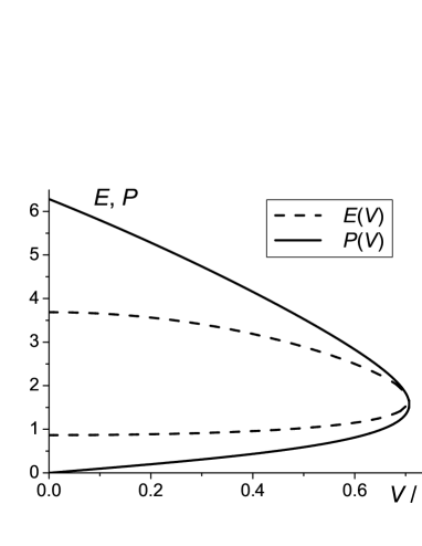
Figure 3: The dependence of the DW energy (in units $JS^{2}$) and its momentum (in units $\hbar S/a$) on its velocity for the value of $h=0.5$.

In the three-dimensional ferromagnet the UDW is unstable. However, this instability develops as an inhomogeneous perturbation (in the plane of the DW) and is not present for DW’s in one-dimensional magnets. Below we will show that for the more natural representation of the DW energy, namely as a function of its momentum, the function $E(P)$ is single-valued, and the upper branch just corresponds to the larger values of momentum. This explains its stability in the one-dimensional case.

The kink momentum is determined as the total field momentum of the magnetization field,Haldane86 , i.e.

$$P=-\int d\xi\;\frac{\delta\mathcal{L}}{\delta\dot{\vec{S}}}\;\vec{S}^{\prime}=-\int\frac{1}{a}\,\vec{A}\,d\vec{S}.$$ (20)

The dynamical part of the Lagrangian in Eq. (9) and the expression (20) for the momentum display singularities associated with the singular behavior of the vector potential $\vec{A}$. The vector potential for a monopole inevitably has a singularity on a line (Dirac string) and moreover is not invariant with respect to gauge transformations. The kink momentum also seems not to be invariant under these gauge transformations. If one uses a Lagrangian written in angular variables, problems due to the non-differentiability of the azimuthal angle $\varphi$ at the points $\theta=0$ and $\theta=\pi$ appear. (This problem is also important for the theory of moving two-dimensional topological solitons, see Ref. papaniko, ). It is important, however, that the difference of the momenta for two different states of the DW is a gauge-invariant quantity.GalkinaIv00 To show this, let us imagine the DW as a trajectory in spin space $\{\vec{S}\}$, $\vec{S}=\vec{S}(\xi)$. The trajectories emerging from one point, say, $\vec{S}=S(\vec{e}_{x}\sin\theta_{0}-\vec{e}_{z}\cos\theta_{0}$) and ending at another point $\vec{S}=S(\vec{e}_{x}\sin\theta_{0}+\vec{e}_{z}\cos\theta_{0}$) can be associated with DW’s that move with different velocities but obey identical boundary conditions at infinity. In this case, the kink momenta are determined by integrals of the form $\int\vec{A}\,d\vec{S}$ along these trajectories. It is clear that the difference of the momenta is determined by the integral $\oint\vec{A}\,d\vec{S}$ along a closed contour. According to Stokes integral theorem, the integral in question can be represented as the flux of the vector $\vec{B}=\;\text{curl}\vec{A}$ through the surface bounded by this contour, $\int\vec{B}\;d{\vec{\Omega}}$. Here the integral is taken over that region on a sphere which is bounded by the trajectories corresponding to the two kinks in question. The vector $\vec{B}=\;\text{curl}\vec{A}=\vec{S}/|\vec{S}|^{3}$ involves no singularities. Returning to angular variables, this difference can be written as $(\hbar S/a)\cdot\int\sin\theta\,d\theta\,d\varphi$, that is just the area on the sphere. Thus, the dependence $V(P)$ or $E(P)$ has been reconstructed, apart from the arbitrariness to choose the reference point for the momenta.

The trajectories describing $v=0$ kinks appear to belong to the large circle passing through the poles $\theta=0,\ \pi$ and the end point of the magnetic field vector $\vec{H}$. Obviously, the difference of the momenta $P$ for the immobile LDW and UDW is determined by the area of the half-sphere, $\Delta P=2\pi\hbar S/a$. All the remaining trajectories that correspond to moving kinks cover the regions between these trajectories. In particular, kinks at the critical velocities $\pm v_{c}$ correspond to two non-planar trajectories. The $v=\pm v_{c}$ trajectories can be reached by proceeding from either type of $v=0$ domain walls, LDW or UDW. Thus, we can see that $E(v)$ has two branches, one characterized by a higher energy and the other characterized by a lower energy. These two branches merge at the critical velocity $v=v_{c}$. If we assume $P=0$ for the $v=0$ LDW, then the momentum grows up to $P=\pm P_{c},\;P_{c}<2\pi\hbar S/a$ as the absolute value of the kink velocity increases to $v_{c}$. As we proceed further along the upper branch of the dependence $E(V)$, the kink velocity decreases, while the momentum increases further to $P=\pm 2\pi\hbar S/a$ when the velocity approaches again zero. When we continue, we begin to cover the area of the sphere once more and the momentum $P$ grows, while the kink energy takes the same values as before: thus we do indeed arrive at a periodic dependence $E(P)$ with period $P_{0}$ determined by the total area of the sphere. The value of $P_{0}$ depends only on the spin value $S$ and the lattice spacing $a$,

$$P_{0}=\frac{4\pi\hbar S}{a}.$$ (21)

The presence of two planar solutions (with $\varphi=\text{const}$) describing the DW’s with $v=0$ and different energies is a common feature for any model with uniaxial anisotropy subject to a transverse magnetic field. As we know, for Heisenberg exchange interaction and single-ion anisotropy, only numerical solutions describing mobile DW‘s can be found.IvKulagin But even in this case the periodicity continues to be the same. On the other hand, for the Ising model considered here, the exact solution is known, and the momentum can be calculated explicitly. As a result the momentum for LDW and UDW takes the following form

$$P_{lower} = \frac{2\hbar S}{a}\arcsin\left(\frac{v}{v_{c}}\sqrt{\frac{1-h^{2}}{1-v^{2}/2}}\right)-$$ (22)

$$- \frac{v\hbar S\sqrt{2}}{a}\arcsin\sqrt{\frac{1-h^{2}}{1-v^{2}/2}}$$

$$P_{upper}=P_{lower}+\frac{4\hbar S}{a}\sqrt{1-\frac{v^{2}}{2}}\cdot\arcsin\sqrt{1-\frac{v^{2}}{v_{c}^{2}}}.$$ (23)

These equations together with Eqs. (17, 18) give us the dispersion law for the DW in implicit form as shown in Fig. 4.

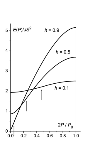
Figure 4: The dependence of the DW energy on its momentum for different values of the magnetic field (given next to the curves); arrows indicate the position of the momentum corresponding to the critical velocity $v_{c}$.

For the mostly interesting case of small magnetic fields $h\ll 1$, or $v\leq v_{c}\ll v_{0}$ the dependence $P(v)$ can be given as the unified expression

$$P_{l,\ u}=\frac{2\hbar S}{a}\left(\frac{\pi}{2}\pm\arcsin\sqrt{1-\frac{v^{2}}{v_{c}^{2}}}\right),$$ (24)

where $\pm$ correspond to UDW and LDW, respectively. Finally, limiting ourselves to the case $h\ll 1$, the dispersion law for both DW’s takes the form

$$E(P)=\sqrt{2}JS^{2}\left[\frac{\pi}{2}-2h\cos\left(\frac{2\pi P}{P_{0}}\right)\right]$$ (25)

This equation will be used in the remaining part of the paper to describe the classical dynamics of domain walls and to perform their semiclassical quantization. It is based on the continuum approximation and this is the only conceivable approach to analytically describe moving DW’s; however, the validity of the continuum approximation has to be justified before doing so since it seems to be non-adequate for the Ising model ferromagnet. This applies in particular to the limit $h\ll 1$, when the DW thickness becomes comparable or even less than the lattice spacing $a$. To check the applicability of the continuum approximation we present in Fig. 5 a comparison of the DW energies as obtained from the numerical approach to those obtained from Eq. (25) at $P=0$. The discrepancy is seen to be of the order of $10\%$ for $h\rightarrow 0$ and thus surprisingly small. In addition, the linear dependence of the DW energy on the magnetic field, $E(H)=JS^{2}(A\pm hB)$ is valid for both approaches, with values $A\approx 2.0$ and $B\approx 2.0$ for the numerical data and $A=\pi/\sqrt{2}\approx 2.2$ and $B=2\sqrt{2}\approx 2.8$ from Eq. (25). As we will see below, the use of the dependence $E(P)=JS^{2}[A-hB\cos(2\pi P/P_{0})]$, with ”improved” coefficients $A$ and $B$, gives much better agreement with the numerical data for the dispersion law of quantum solitons.mik-miyash

One more important parameter, the maximum value of the pinning potential $U_{0}$ was treated numerically for arbitrary values of $h$. For extremely small values of $h$, $U_{0}=E_{CB}-E_{CS}=2JS^{2}h[1-3(h/2)^{1/3}]$ was obtained from the analytical expressions for $E_{CS}$ and $E_{CB}$ (see Eqs. (11,12) in Ref. mik-miyash, ). As we will see below, the ratio of $U_{0}$ to the difference of the DW energies with $P=0$ and $P=P_{0}/2$, $T_{0}=JS^{2}hB$ is an important parameter for the description of the DW dynamics. Whereas the dependence of $U_{0}$ on $h$ is non-linear at small values of $h$ because of the presence of the non-analytical term proportional to $h^{1/3}$, the DW ”kinetic energy” $T_{0}$, is linear in $h$, see Sec. V below. The maximum value of $U_{0}/T_{0}=1/2$ is realized in the limit $h\rightarrow 0$, but in fact this important ratio decreases fast to rather small values when $h$ grows (see Fig. 6).

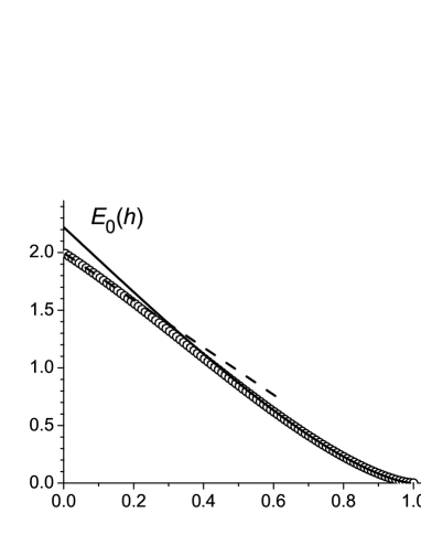
Figure 5: The dependence of the DW energy with zero velocity (in units $JS^{2}$) on the dimensionless magnetic field $h$; symbols depict the numerical data for the discrete model; the solid line is the theoretical result in the continuum approximation Eq. (25); the approximation of numerical data by the linear function $E=2(1-h)JS^{2}$ is shown as dashed line.

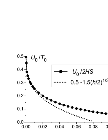
Figure 6: The ratio of the maximum value of the pinning potential to the quantity $T_{0}$ characterizing the dispersion of the DW. For $T_{0}$, the ”improved” value of the coefficient $B=2$ is used. Also shown as dotted line is the limit of this quantity for extremely small values of the magnetic fields mik-miyash , $U_{0}/T_{0}=0.5[1-3(h/2)^{1/3}]$.

In the limit of small values of momentum, $P\rightarrow 0$, the parabolic approximation can be used and the energy takes the form $E=P^{2}/2M$, where the effective mass of a kink is

$$M=\frac{4\sqrt{2}\hbar^{2}}{a^{2}hJ}.$$ (26)

It is seen from Eq. (26) that the effective mass turns to infinity at $h\rightarrow 0$. This is one more manifestation that in a purely uniaxial model of a ferromagnet in the absence of a transverse magnetic field domain wall motion is impossible.IvKulagin The use of the parabolic approximation (26) seems to be adequate for DW’s moving with small velocities. However, some important features are lost in this approximation: For example, the correct value of the energy bands forming the DW spectrum should be found within the analysis of the full periodic dependence $E(P)$.

We note that for small $h$ the value of the effective mass for the upper DW branch, defined by $E_{upper}(P)=E(P_{0}/2)-(P-P_{0})^{2}/2M_{up}$ agrees with $M$ from Eq. (26). However, $M$ and $M_{up}$ are substantially different at finite $h$, see Fig. 4 above.

To conclude this section, we emphasize that within the macroscopic classical approach the dispersion law (25) exhibits a periodic dependence of $E(P)$ which, from Bloch’s theorem, is characteristic for discrete quantum models. Moreover the maximum value of momentum, $P_{0}=4\pi\hbar S/a$, which may be called the size of magnetic Brillouin zone, and the size on the crystalline Brillouin zone $P_{B}=2\pi\hbar/a$ have values of the same order at $S\sim 1$. The expression for $P_{0}$ contains Planck’s constant $\hbar$ and the lattice constant $a$ and formally seems to characterize both the quantum nature and the discreteness of the model. As discussed above, this is not the case: if one accounts for the macroscopic (continuous) character of the magnetization $M_{0}=g\mu_{B}S/a$ (otherwise the discussion of ferromagnetism is meaningless), $P_{0}$ can be written using only $M_{0}$ and the classical gyromagnetic ratio $\gamma=e/2mc,P_{0}=4\pi M_{0}/g\gamma$.

IV Forced motion and dispersion relation of domain walls

The periodic dependence discussed in the preceding section means that one can restrict the values of momentum $P$ to the magnetic Brillouin zone, $-P_{0}/2<P<P_{0}/2$. On the other hand, as with Bloch electrons, in order to analyze the motion under the influence of an external force, it is useful to consider that the DW momentum obeys the equation $dP/dt=F_{e}$, where $F_{e}$ is external force, and to allow that $P$ increases without limits beyond the first Brillouin zone. The expression for the DW energy $E(P)$ can be used to describe the DW dynamics in the spin chain in terms of the DW coordinate $X$ considered as a collective variable. Its dynamics is governed by the Hamiltonian

$$\mathcal{H}(P,X)=E_{0}(h)+T_{0}\sin^{2}(\frac{\pi P}{P_{0}})+U(X),$$ (27)

where $E_{0}(h)$ is the DW energy at $P=0$. $E_{0}(h)$ has no effect on the dynamics of the DW coordinate $X$ and will be omitted below. Here we have introduced the parameter

$$T_{0}=4\sqrt{2}hJS^{2}=2\sqrt{2}g\mu_{0}SH$$

which describes the magnitude of free DW dispersion, and added the potential $U(X)$, without specifying its physical origin. For the discrete spin chain, the potential is the pinning potential originating from the discreteness effects introduced above.

It is easily seen that the relation $\dot{X}\equiv V=\partial\mathcal{H}/\partial P$ as in analytical mechanics immediately gives the periodic (oscillating) dependence of the DW velocity on DW momentum

$$V=\frac{\pi T_{0}}{P_{0}}\sin(\frac{2\pi P}{P_{0}})$$ (28)

Inverting this equation we recover the expression for the momentum (24) for small magnetic field.

The dynamical equation for the Hamiltonian reads $dP/dt=-\partial\mathcal{H}/\partial X$. Choosing different forms of the potential $U=U(X)$ one can consider different problems such as the interaction between a DW and the inhomogeneities in the medium or with external magnetic field $H_{z}$ directed along the easy axis. In the last case we have

$$U(X)=-2g\mu_{B}SH_{z}\cdot X/a,\ \text{and}\ \dot{P}=2g\mu_{B}H_{z}S/a.$$ (29)

Therefore the DW velocity under the action of constant magnetic field (constant force) oscillates with time. Note that for a DW in the uniaxial ferromagnet this equation is nothing but the one-dimensional version of familiar Slonczewsky equations.malslon It describes the nontrivial properties of DW dynamics, such as the oscillating motion of DW’s as response to a constant external force. These effects were observed in a number of experiments on DW dynamics in bubble-materials, see Ref. malslon, . Formally, such a motion corresponds to the Bloch oscillations well known for quantum mechanical electron in an ideal crystal lattice. Bloch oscillations for solitons in different media were recently reviewed by Kosevich.Kosevich01 Also, such effects for DW’s in spin chains with $S=1/2$ have been discussed from the viewpoint of Bloch particles recently.KirLoss98 However, it is important to note that for DW’s in a continuum model the origin of the effects is different in principle: It is not associated with discreteness and it exists even in the continuum limit. Thus, even in the classical continuum model the dynamics of a DW exhibits a number of properties peculiar to Bloch particles (electrons), i.e. to quantum objects moving in the periodic potential of the crystal lattice. On the other hand, the time dependence of this forced DW velocity is oscillating with the classical Larmor frequency $\Omega_{L}=g\gamma H_{z}$. Combining Eqs. (28) and (29) one can find

$$V(t)=V_{max}\sin\Omega_{L}t,\ V_{max}=\pi T_{0}/P_{0}.$$

Thus, the quantum and classical regularities intertwine in a very intricate manner in the problem of domain wall dynamics.

To analyze the quantum DW motion in the spin chain including discreteness effects, we will use Eq. (27) as a quantum Hamiltonian, using the periodic potential of Eq. (4) and $U_{0}$ as found in the Sec. II. Let us start with the case of nearly free motion, when $U_{0}\ll T_{0}$. In this case the DW energy is given not by the usual momentum, but instead by the quasi-momentum $P$ which is determined only up to a reciprocal lattice vector. According to Bloch’s theorem, the energy $E(P)$ should be periodic with period $P_{B}=2\pi\hbar/a$. When $U_{0}\rightarrow 0$, the dispersion law is described by Eq. (25), or Eq. (27) with $U_{0}=0$, for almost all $P$ values (with small corrections $\sim U_{0}^{2}$). Only when the non-perturbed dispersion laws intersect, $E(P)=E(P+nP_{B})$ with $n$ integer, corrections become essential $(\sim U_{0})$ and energy gaps appear.

We now want to discuss the situation for different values of spin $S$, since the ratio $P_{0}/P_{B}=2S$ depends on the spin value. Strictly speaking, small spin values, e.g. $S=1/2,\ 1,...$, cannot be described in the frame of our semiclassical approach. But we argue that our approach will be valid at least qualitatively also for these cases.

For spin $S=1/2$ we have $P_{0}=P_{B}$, and there is no intersection of the non-perturbed dispersion law with its image shifted by $P_{B}$ (the intersection of two parabolas in Ref. br-loss, is an artefact of the parabolic approximation). In this case the effect of small $U(X)$ on the DW dispersion relation $E(P)$ is only quadratic in the small parameter $U_{0}$ and is negligibly small. For all other spin values, $S>1/2$, we have $P_{0}>P_{B}$ and dispersion curves $E_{0}(P)$ extended periodically with period $P_{B}=2\pi\hbar/a$ do intersect. However, all intersections occur on the boundaries of the Brillouin zone, namely, at $P=\pm\pi\hbar/a$. It is clear that in this case the DW spectrum contains $N_{b}=2S$ energy bands.

V Classical dynamics of domain walls in a finite potential and its quantization

In this section we will analyze the classical DW dynamics and its quantization for an arbitrary (finite) periodic potential of the form given in Eq. (4). The most important ingredient to this analysis is that the Hamiltonian of Eq. (27), just as the classical energy, is a periodic function of momentum, and that there is an upper bound for the energy. As already mentioned, this property is already present in the classical theory of DW motion and has nothing to do with quantum mechanics. We will show below that this property leads to results which are qualitatively different from those obtained in the standard quadratic approximation, both for the pure classical DW motion as well as for its quantization.

Let us consider the dynamical system described by the classical Hamiltonian of Eq. (27), taking $U(X)$ into account. The corresponding Hamilton equations

$$\frac{\partial P}{\partial t}=-\frac{\partial\mathcal{H}}{\partial X},\;\frac{\partial X}{\partial t}=\frac{\partial\mathcal{H}}{\partial P},$$

have an obvious integral of motion,

$$\mathcal{H}(P,X)=T_{0}\sin^{2}\frac{\pi P}{P_{0}}+U_{0}\sin^{2}\frac{\pi X}{a}=\text{const}.$$ (30)

Here we have omitted the constant part $E_{0}(h)$ which does not affect the equations of motion. These equations cannot be integrated in terms of elementary functions, however, a sufficiently complete understanding of the DW dynamics can be found using the phase plane analysis. This system is characterized by the periodicity in momentum $P$ and by the presence of an upper bound for the Hamiltonian. In view of this its dynamics shows characteristic features which do not manifest themselves for standard dynamic systems with a parabolic dependence on momentum.

It is easy to show that at arbitrary $U_{0}/T_{0}$ there are two sets of center-like singular points in the phase plane, see Fig. 7. One of them ($C1-$type center) corresponds to the minimum of the potential $U(X)$ and the minimum of the ”kinetic energy” $T(P)=T_{0}\sin^{2}(\pi P/P_{0})$,

$$C1:X=an,\ P=P_{0}m,\ \mathcal{H}_{C1}=0,\hfill$$

the other set of centers ($C2-$type center) is located at the maximum of both potential and kinetic energies,

$$C2:\ X=a(2n+1)/2,\ P=P_{0}(2m+1)/2,\ \mathcal{H}_{C2}=U_{0}+T_{0}.$$

Here and below $n,m$ are integers. The existence of $C2-$type centers describing the steady small oscillations of the UDW near the potential maximum, is a unique property of Hamiltonian systems with an upper bound in the Hamilton function $\mathcal{H}(P,X)$.

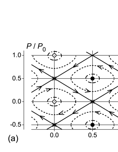
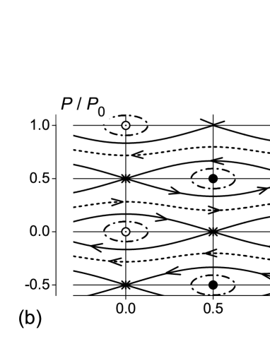
Figure 7: The phase plane $(P,X)$ for the DW dynamics for (a) $U_{0}=T_{0}$ and (b) $U_{0}=0.25T_{0}$. Separatrix trajectories are shown by full lines, other trajectories by dashed lines; full and open circles denote the positions of center-like singular points $C1$ and $C2$, crosses correspond to the saddle points.

There are also two sets of saddle points in the phase plane, $S1$ and $S2$. Points $S1$ correspond to the maxima of the potential $U(X)$ and the minima of $T(P)$

$$S1;\ X=a(2n+1)/2,\ P=P_{0}m,\ \mathcal{H}_{S1}=U_{0},$$

points $S2$ correspond to the minima of $U(X)$ and the maxima of $T(P)$,

$$S2;\ X=an,\ P=P_{0}(2m+1)/2,\ \mathcal{H}_{S2}=T_{0}.$$

At the allowed values of the integral of motion, $\mathcal{H}_{C1}\leq\mathcal{H}\leq\mathcal{H}_{C2}$, the phase plane $(P,X)$ separates into regions with different types of motion. Two types of finite motion are present within one interatomic distance (one period of the potential). One type of finite motion corresponds to the oscillations of the LDW near the minimum of the potential, it requires $\mathcal{H}_{C1}\leq\mathcal{H}\leq\mathcal{H}_{S1}$ and is standard in the analytical dynamics of a particle. (We suggested $U_{0}\leq T_{0}$ here). A second type of finite motion, namely oscillations of the UDW near the potential maximum, is realized for $\mathcal{H}_{S2}\leq\mathcal{H}\leq\mathcal{H}_{C2}$. These regimes are separated from the rest of the phase plane with different types of infinite motion by separatrix trajectories, ending in one of the saddle points. The only exception is the case $U_{0}=T_{0}$ or $\mathcal{H}_{S1}=\mathcal{H}_{S2}$ when the separatrix trajectories connect saddle points of different type and form a two-dimensional net; as a consequence infinite motion is absent. For the transverse field Ising model with small $U_{0}$ this is hard to realize, see Sec. II (in particular Fig. 6), but for methodological purposes we find it convenient to start with this case.

In this case we have $T_{0}=U_{0}$, and one easily verifies that the area of the phase plane (mechanical action) per unit cell and one period of momentum is equal to $\mathcal{A}_{0}=4\pi\hbar S$. Thus, from the Bohr-Sommerfeld quantization rules, there are ($\mathcal{A}_{0}/2\pi\hbar)=2S$ quantum eigenstates of a DW, related to its oscillations per one unit cell. It is clear that if one takes into account tunneling transitions between equivalent points of the lattice, these localized states will turn into energy bands.

This result coincides with the result obtained in the previous section for the opposite limit of an infinitely weak pinning potential. An additional argument on the number of energy bands is obtained from the well-known exact result for so-called Harper equation,harper familiar in the problem of electronic quantum motion in a periodic potential in the presence of a finite magnetic field. In accordance with Ref. harper, the problem is reduced to a Hamiltonian as in Eq. (30), ${\mathcal{H}}_{H}=\sin^{2}(p/2)+\sin^{2}(\pi\beta q)$. For the rational case of the Harper equation, at $\beta=m/n$, the eigenvalue spectrum for the Hamiltonian ${\mathcal{H}}_{H}$ shows $n$ non-overlapping bands. The simple canonical transformation $p\rightarrow\pi P/P_{0},\ q\rightarrow XP_{0}/\pi$, leads to our Hamiltonian (30) with $\beta=1/2S$. This gives immediately the above result, $N_{b}=2S$.

For $T_{0}<U_{0}$, a case more realistic for the Ising model, the situation is different: in addition to the localized trajectories in phase space, trajectories corresponding to the infinite motion above the potential barrier appear, see Fig. 7b. These trajectories describe the overbarrier dynamics of DW’s in the pinning potential. It is clear, that such states should be described well by the model of the nearly-free particle, discussed in the previous section.

The other limiting case, large $U_{0}$, i.e. $U_{0}>T_{0}$ is hard to realize in the transverse field Ising model. On the other hand, it could be interesting for other models of ferromagnets supporting DW states, and we want to discuss it briefly. The phase plane for large $U_{0}/T_{0}$ can be obtained from Fig. 7b by replacing $P/P_{0}$ by $x/a$ and vise versa. Then, the topology of the phase plane is fundamentally changed: trajectories with finite changes of the kink coordinate and infinite range in momentum, appear. For these trajectories the DW coordinate oscillates near certain positions, which do not coincide with a minimum or maximum of the pinning potential. This is nothing but Bloch oscillations in the pinning potential $U(X)$.

At this point we want to emphasize that the semiclassical result $\mathcal{A}_{0}=4\pi\hbar S$ does not depend on the details of the model. Only the periodicities of the Hamiltonian in $P$ and $X$ with periods $P_{0}$ and $a$ are essential for the argument. The considerations presented in the previous section are model independent as well, and lead to the same value of $P_{0}$ for all transverse field models. Therefore the final result for the number of energy bands remains valid for more general models of ferromagnets subject to a transverse magnetic field. Thus the number $N_{b}$ of energy bands for DW’s in all these models should be equal to $2S$. This is in agreement with the numerical result for the kink dispersion law in the quantum transverse field Ising model with spin $S=5$, where 10 energy bands were obtained. mik-miyash

VI DW tunneling

In the classical case, there are states corresponding to finite motion (oscillations) of DW’s near the extrema of the potential in the phase plane both at small and large values of $U_{0}$. This applies to the LDW near the minimum of $U(X)$ and as well to the UDW near the maximum of $U(X)$. Owing to the symmetry present in the Hamiltonian (30), $P\rightarrow P_{0}/2-P$, $X\rightarrow a/2-X$, their dynamics is described similarly; therefore one can consider only, say, the LDW case. In the quantum case, the tunneling of DW’s from one site to another becomes possible, and these states form the energy bands. It is clear that for extremely small $U_{0}$ the nearly free approximation discussed in section IV is valid. But the standard situation for semiclassical systems (like DW’s for large spin ferromagnets) is the tight-binding limit, for which the probability of tunneling is small, and the states with energy $E_{n}$ are almost localized in a potential well. In order to estimate $E_{n}$, we consider the parabolic approximation for both $U(X)$ and $T(P)$. In this case we have $E_{n}=\hbar\omega_{0}\cdot n$, where

$$\omega_{0}=\sqrt{\frac{1}{M}\left(\frac{d^{2}U}{dx^{2}}\right)_{X=0}}=\frac{\sqrt{U_{0}T_{0}}}{4\hbar S}.$$

$M$ is the effective mass of Eq. (26). Both $U_{0}$ and $T_{0}$ are proportional to $S^{2}$, therefore $\omega_{0}\propto S$ and for semiclassical spins $S\gg 1$ the value of $E_{n}$ for $n\ll S$ can be smaller than $U_{0}$ even in the case $U_{0}\ll T_{0}$. Then the width of the $n^{\rm th}$ energy band, $\Delta E_{n}$, resulting from the tunneling between the quantized energy levels $E_{n}$, is smaller that the value of $T_{0}$ and even $E_{n}$. It is clear that this first of all should correspond to the lowest level $E_{n}$, i.e. $n=0$ (the ”ground state of the DW” in the pinning potential), but it could be true as well for some higher levels with $n>1$.

In order to understand the possibility of semiclassical dynamics of the lower DW, consider the limit of small $U_{0}$, $(U_{0}\ll T_{0})$. The area $\mathcal{A}_{L}$ under the separatrix trajectories $S1$ is easily found and the number of quantum states for the finite motion of the LDW, $N_{L}=\mathcal{A}_{L}/2\pi\hbar$ is defined by the following expression

$$N_{L}=\frac{8S}{\pi^{2}}\sqrt{\frac{U_{0}}{T_{0}}}.$$

This is of the same order of magnitude as the value obtained from $N_{L}\cdot\hbar\omega_{0}=U_{0}$. The same expression is obtained for the number of states of the upper DW, localized near the potential maximum, $N_{U}=N_{L}$. At $U_{0}\ll T_{0}$, the values of $N_{U}$ and $N_{L}$ are much smaller than the total number of DW states $2S$, but can still be large compared to 1: When the inequality

$$\frac{1}{S^{2}}\ll\frac{U_{0}}{T_{0}}\ll 1,$$

(meaningful for $S\gg 1$) holds, the states of finite motion are a small fraction of all DW states, but $N_{U}=N_{L}\gg 1$. It is easy to estimate the mean values of $P^{2}$ and $X^{2}$ in these states,

$$\left\langle P^{2}\right\rangle=P_{0}^{2}\cdot\frac{1}{2\pi S}\sqrt{\frac{U_{0}}{T_{0}}},\;\;\left\langle X^{2}\right\rangle=a^{2}\cdot\frac{1}{2\pi S}\sqrt{\frac{T_{0}}{U_{0}}}.$$

In view of that, it is not easy to satisfy the condition of applicability of the parabolic approximation for both $U(X)$ and $T(P)$, $\left\langle P^{2}\right\rangle\ll(P_{0}^{2})$ and $\left\langle X^{2}\right\rangle\ll a^{2}$ simultaneously. Thus, in order to investigate the tunneling splitting of the levels it is preferable to use the full non-parabolic Hamiltonian Eq. (30). The best way to analyze such models is the instanton technique, which can be applied for arbitrary field theories, see Ref. Rajaraman, . In this approach, the amplitude of probability $\mathcal{P}_{12}$ of the transition of the DW from one given state to another is determined by the path integral $\int DX\cdot\exp\{i{\mathcal{A}}[X]/\hbar\}$, where ${\mathcal{A}}[X]=\int dt\cdot{\mathcal{L}}[X(t)]$ is the mechanical action functional. Here ${\mathcal{L}}(X,\ \dot{X})$ is the Lagrangian describing the dynamics of the DW coordinate $X$, and the integration $DX$ goes over all configurations $X(t)$ satisfying the given boundary conditions. The Lagrangian ${\mathcal{L}}(X,\ \dot{X})$ is easily obtained, as in standard mechanics, from ${\mathcal{L}}=P\dot{X}-{\mathcal{H}}$: express $P$ and ${\mathcal{H}}$ in terms of $\dot{X}$, using the known expressions for $P=P(V)$ and ${\mathcal{H}}=E(V)+U(X)$ (see section III), replacing $V$ by $\dot{X}$.

It is convenient to make a Wick rotation $t\to i\tau$, passing to the Euclidean space-time. Then one has the Euclidean propagator $\int DX\,\exp[-{\mathcal{A}}_{E}/\hbar]$, where the Euclidean action is written as

$${\mathcal{A}}_{E}=\int{\mathcal{L}}_{E}(X,\Omega)d\tau,$$

with $\Omega=dX/d\tau$. For the LDW this gives

$${\mathcal{L}}_{E}=\frac{2\hbar S}{a}\left[\Omega\text{arcsinh}\left(\frac{\Omega}{V_{c}}\right)+V_{c}-\sqrt{V^{2}_{c}+\Omega^{2}}\right]+U(X).$$ (31)

Constructing the instanton solution can then be viewed as minimization of ${\mathcal{A}}_{E}$ with respect to $X(\tau)$. The minimum of the Euclidean action is realized on the solution of the Euler-Lagrange equation for ${\mathcal{L}}_{E}$. The first integral of this equation has the form

$$\frac{2\hbar S}{a}\left(\sqrt{V_{c}^{2}+\Omega^{2}}-V_{c}\right)-U(X)={\mathcal{C}},$$

with ${\mathcal{C}}=0$ on the instanton solution. Then, the expression for ${\mathcal{A}_{E}}$ reduces to the integral

$${\mathcal{A}}_{E}=\frac{2\hbar S}{a}\int_{0}^{a}\text{arcsinh}(\frac{\Omega}{V_{c}})dX,$$

which has to be calculated using the connection between $\Omega$ and $X$ from the first integral, $(\Omega T_{0}/V_{c})^{2}=4U(X)[T_{0}+U(X)]$. Finally, the expression for the Euclidean action on the instanton solution takes the form

$$\frac{{\mathcal{A}}_{E}}{\hbar}=\frac{8S\sqrt{U_{0}}}{\pi}\cdot\int_{0}^{\pi/2}\frac{\psi d\psi\sin\psi}{\sqrt{T_{0}+U_{0}\sin^{2}\psi}}.$$ (32)

For the most natural case $U_{0}\ll T_{0}$ this gives the result

$${\mathcal{A}}_{E}^{(0)}=\frac{8\hbar S}{\pi}\cdot\sqrt{\frac{U_{0}}{T_{0}}}\ \text{at}\ U_{0}\ll T_{0},$$ (33)

as usual for a Lagrangian with quadratic dependence on the velocity. For arbitrary $U_{0}/T_{0}$ the calculations are more complicated but the tendency is seen as follows: ${\mathcal{A}}_{E}$ is smaller than predicted by Eq. (33) for the same value of $U_{0}/T_{0}$, see Fig. 8. Thus, the band width for finite $U_{0}/T_{0}$ is larger than follows from Eq. (33).

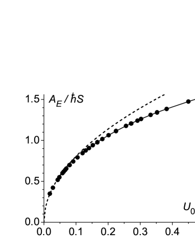
Figure 8: The dependence of the Euclidean action on the value of $U_{0}/T_{0}$ as found numerically (symbols) and from the asymptotic Eq. (33), $A_{E}\propto\sqrt{U_{0}/T_{0}}$, valid for small $U_{0}/T_{0}$ (dotted line). The maximum value of $A_{E}/\hbar S=1.533$ is reached at $U_{0}/T_{0}=0.5$, that is the maximum value of $U_{0}/T_{0}$ for the transverse field Ising model.

For energy bands $\Delta E_{n}$ with $1\ll n\ll N_{L}$ and $U_{0}\ll T_{0}$ we can use the fact that in the regime of classical motion the simple parabolic dispersion law is valid to calculate the tunneling splitting of the levels. This allows to use the standard expression for the tunnel splitting of the levels (see Ref. quantum mech, , problem 3 after §50) and results in

$$\Delta E=(\hbar\omega_{0}/\pi)\exp\left\{-\int_{-a^{\prime}}^{+a^{\prime}}\{2m[U(X)-E]\}^{1/2}dX/\hbar\right\}.$$

Here $a^{\prime}$ is the turnover point of the classical trajectory with energy $E_{n}$ (corresponding to a non-split level) defined by the equation $U(a^{\prime})=E$. It is convenient to rewrite it using the Euclidean action only. After some simple algebra we arrive at the following universal formula:

$$\Delta E_{n}\simeq\hbar\omega_{0}\left(\frac{{\mathcal{A}}_{E}}{\hbar}\right)^{n+1/2}\cdot\exp\left(-\frac{{\mathcal{A}}_{E}}{\hbar}\right)\ ,$$ (34)

where ${\mathcal{A}_{E}}$ is given by Eq. (32) or Eq. (33), with ${\mathcal{A}_{E}}\propto S$ in both cases. This equation shows that the energy splitting for $n>1$ continues to be exponentially small in $S$, but with larger pre-exponential factor. This is in good agreement with numerical data.mik-miyash

VII Summary and discussion.

We start this summary with the explicit results obtained for the transverse field Ising model, and then go on to discuss the conclusions which might be obtained for more general models. The characteristic feature of the Ising model is that the two important parameters $U_{0}$ and $T_{0}$ of the theory are governed by only one quantity, the dimensionless magnetic field $h$; practically always $U_{0}\ll T_{0}$ holds. However, the behavior of the quantum DW spectrum depends also on the value of the atomic spin $S$. If $U_{0}\ll T_{0}$, but $S^{2}>T_{0}/U_{0}$, top and bottom energy bands are very narrow. The neighboring bands are narrow also, but $S$ timer wider, and the intermediate part of the spectrum consists of wide bands with narrow energy gaps. This picture corresponds well with the numerical data for the model with $S=5$ of Ref. mik-miyash, (see Fig. 9).

Unfortunately, the direct quantum mechanical approach used in Ref. mik-miyash, can be applied for small values of $h$ only; then the discreteness effects are large and the continuum approximation is not appropriate. But the discrepancies are not too large, and even in this unfavorable situation we can claim at least qualitative agreement. The data are fitted quantitatively only with use of fitted dependence $E(h)$ (see end of Sec. II and Fig. 6). It is worth to mention that there are at least two reasons for discrepancies, caused by (i) nonapplicability of the continuum limit to the small field discrete classical Ising model, and (ii) the fact that the Landau-Lifshitz equation is not adequate to describe quantum DW’s. We believe that discreteness is the main source of the discrepancy, and for models with wide enough DW’s, (such as models of ferromagnets with nearly-isotropic exchange interaction and weak magnetic anisotropy), the description of quantum dynamics of DW’s based on the scheme proposed in this paper will be at least semi-quantitative.

Figure 9: The dependence of the DW energy on its momentum for the magnetic field $h=0.05$ as obtained in the continuum approximation. The dashed line presents the result of the continuum approach, the solid line is improved by using the fitted dependence $E(h)$ for small $h$ (see Fig. 5). Symbols show the numerical data for the dispersion law of the quantum DW.mik-miyash

At this point it is interesting to compare the results of the instanton approach with data from an analysis of the model for extremely small field, when spin zero-point fluctuations far from a DW can be neglected and the one-site approximation can be applied.mik-miyash In both approaches the widths of the energy bands with lower energies are exponentially small in the spin magnitude $S$. The one-site approximation yields an exponential factor of the form of $\exp(-2S\ln 2)\approx\exp(-1.39S)$,mik-miyash which is quite close to the value $\exp(-\mathcal{A}_{E}/\hbar)\rightarrow\exp(-1.53S)$ at $h\rightarrow 0$, obtained in the instanton approach using improved data for $T_{0}$, $U_{0}/T_{0}\rightarrow 1/2$. It is interesting to note that using the data obtained directly from the continuum approximation, $U_{0}/T_{0}=1/(2\sqrt{2})$, the factor takes the form $\exp(-1.34S)$ which is much closer to the value obtained in Ref. mik-miyash, . The agreement between the data can be considered rather good, regarding the conceptual difference between the two approaches.

Good agreement is also found with respect to the fact that the band width increases with energy, the ratio of the widths of neighbouring energy bands is given by a factor of $S$. But the pre-exponential factors for these, essentially alternative, approaches differ by a factor of $\sqrt{S}$. It is most likely that taking into account fluctuations far from the DW center becomes essential for the determination of the pre-exponential factor. It is worth noting the formal agreement that, within the instanton approach, this factor is determined by the fluctuation determinant only, again, far from the instanton center. Again, the compliance of data of these two approaches can be considered as satisfactory.

The instanton analysis demonstrates that while the field is increasing, $\mathcal{A}_{E}/\hbar$ very rapidly decreases, see Fig. 8. Thus, the width of the energy band grows rapidly, the gaps become narrow and the nearly-free limit can be realized for all energies. At $S=5$ the value of $\mathcal{A}_{E}/\hbar$ becomes of the order of unity and $\Delta E_{0}\approx\hbar\omega_{0}$ already at $U_{0}/T_{0}<0.008$ (equivalent to the magnetic field becoming close to $h\sim 0.3$). But for any values of the parameter $h$, $2S$ energy bands are present in the DW spectrum. As we argued above, this result is not specific to the Ising model. It is mostly due to the value of the period $P_{0}$, which is universal for all models of uniaxial ferromagnets in a transverse magnetic field. Thus, the result that 2$S$ energy bands exist should be valid for all transverse field models of ferromagnets.

The results obtained here for ferromagnets can be applied to Ising antiferromagnets as well. The simple canonical transformation

$$S_{n}^{y,z}\rightarrow(-1)^{n}\sigma_{n}^{y,z},\ S_{n}^{x}\rightarrow\sigma_{n}^{x},$$

results in the same commutation relations for staggered magnetization $\vec{\sigma}_{n}$ as for usual spins $\vec{S}_{n}$ and reproduces the same form for the Hamiltonian, Eq. (1), replacing $\vec{S}_{n}$ by $\vec{\sigma}_{n}$ and changing the sign of $J$. It is easy to prove, after the appropriate gauge transformation, that the form of the Lagrangian, Eq. (10) is also unchanged. Thus, all the results obtained here for the DW dynamics, its dispersion law and its semiclassical quantization are valid for Ising antiferromagnets as well. Note that such a simple connection can be true only for models with a Hamiltonian depending on two components of spin only. This excludes near Heisenberg antiferromagnets. For the near Heisenberg antiferromagnets with weak anisotropy of any origin, exchange or single-ion, treated on the basis of the sigma-model, the singularities in the Lagrangian for the staggered magnetization are absent for a sufficiently general set of models (including antiferromagnets subject to strong external magnetic fields and in the presence of Dzyaloshinski-Moriya interactions of arbitrary symmetry IvKireev2002 ) and a periodic DW dispersion law is not realized.GalkinaIv00

Another interesting feature, which is common to classical and quantum physics, is that states with finite range of motion for the coordinate, but infinite range for momentum are present for large enough pinning potential, $U_{0}>T_{0}$. Evidently such trajectories do not exist for standard mechanical systems with a parabolic dispersion law $\mathcal{H}=P^{2}/2M+U(X)$. Of course the number of quantized states of DW motion per unit cell does not depend on the ratio of $U_{0}$ and $T_{0}$ and remains equal to $2S$. For the case of extremely weak dispersion $T_{0}\ll U_{0}$, it follows that intermediate DW positions in the periodic potential are quantized and are equal to $2S$ discrete values. Thus, in the case of semiclassical quantization of DW motion within the continuum problem, there are $2S$ positions of the DW, i.e. some internal scale, $a_{m}=a/2S$ appears in the problem. This fact might be used to explain intuitively that a magnetic Brillouin zone, $P_{0}=2SP_{B}$, appears (here $P_{B}=2\pi\hbar S/a$ is the size of the Brillouin zone in a chain with interatomic distance $a$). To explain this in a slightly different way, we mention that the DW coordinate is directly connected with the $z-$projection of the total spin $\mathcal{S}_{z,\ tot}$, see (3), and this quantum-mechanical quantity can change by unit steps only.

It is interesting to compare the features established here for transverse field models to the 180-degree DW ($\pi-$kink) in ferromagnets with rhombic anisotropy as considered by Braun and Loss br-loss . For their model there are two different DW’s with lowest energy (Bloch DWs) and the corresponding $\vec{S}(\xi)$ trajectories are the halves of the large circle passing through the easy axis and the axis with the intermediate value of anisotropy.

It is easy to argue, that in this case the dependence $E(P)$ found in the continuum approximation is again periodic, but the period of this dependence $P_{0,\pi}$ is determined by half of the sphere $\vec{S}^{2}=S^{2}$, and it is two times smaller than that for the transverse field model, $P_{0,\pi}=2\pi\hbar S/a$.Sklyanin79 ; Haldane86 ; GalkinaIv00 The specific model treated in br-loss is exactly integrable, and the free dispersion law $E(P)$ with this period can be constructed explicitly, see Refs. sowsci, ; phys.rep, . On the other hand, for the full classification of DW’s, i.e. to describe the presence of two different, but energetically equivalent DW’s one can in this situation introduce the discrete parameter chirality. Braun and Loss have shown from a different argument that the minima of the dispersion laws $E(P)$ for DW’s with different chiralities have to be located at different points of the $P$-axis, with distance equal to $P_{0,\pi}$ (in our terminology). Owing to the parabolic approximation, used in Ref. br-loss, , the dispersion curves $E(P)$ for different chiralities seem to be intersecting in some point. But accounting for the real periodic dependence for $E(P)$, these two minima are smoothly connected, with the maximum at the energy of the Néel DW, and no intersection occurs. Thus, there is no reason for the chirality tunneling to take place in this formulation. The deep connection of chirality and linear momentum and the suppression of quantum tunneling of chirality for free 180-degrees DWs in ferromagnets has been discussed recently by Shibata and Takagi.TakagiShib00 It is worth to note here, that also for 180-degree DW’s in Heisenberg antiferromagnets two non-equivalent DW’s with equal energies are present, but the dependence $E(P)$ is not periodic. Chirality is not connected with the value of linear momentum and the effects of quantum tunneling of chirality are present even without the pinning potential.ivkol

Finally we want to discuss the perturbation of the dispersion law for a 180-degree DW caused by a small periodic pinning potential $U(X)$. For this case, one has to locate the intersections of non-perturbed spectra $E(P)$, periodically extended with period $P_{B}=2\pi\hbar/a$. The situation here is slightly more complicated than for transverse field models: For small spins $S=1/2$ and $S=1$ one has $P_{0,\pi}\leq P_{B}$, intersections are absent and no gaps are present (this is the same situation as for the transverse field model with spin $S=1/2$). For integer spins $S=k,\ k>1$ intersections occur and energy gaps appear at the intersection points. However, all these gaps are located on the boundaries of the Brillouin zone. Then, the number of energy bands is equal to $S$. But for sufficiently large half-integer spins $S=(2k+1)/2,k\geq 1$, one has $P_{0}=P_{B}(2n+1)/2$, and some intersections are inside the Brillouin zone at $P=(2n+1)\pi\hbar/2a$, with integer $n$. This leads to the appearance of some additional gaps, which could be associated with the tunneling of chirality. In this case the number of gaps increases and for half-integer spin $S$ the number of energy bands in the dispersion relation for 180-degree DW’s is equal to $2S$.

- (1) H.-J. Mikeska and M. Steiner, Adv. Phys. 40, 191 (1991).
- (2) V. G. Bar’yakhtar and B. A. Ivanov, in Soviet Scientific Reviews, Section A. Physics, I. M. Khalatnikov (ed.), 16, 3 (1993).
- (3) A. M. Kosevich, B. A. Ivanov, and A. S. Kovalev, Phys. Rep. 194, 117 (1990).
- (4) J. Villain, Physica, B 79, 1 (1975).
- (5) H.-J. Mikeska, S. Miyashita, and G. Ristow, J. Phys.: Condens. Matter, 3, 2985 (1991)
- (6) H. J. Bethe, Z. Phys. 71, 205 (1931).
- (7) R. G.Baxter, Ann. Phys. 70, 323, (1972); J. D. Johnson, S. Krinsky and B. M. McCoy, Phys. Rev. A8, 2526 (1973).
- (8) B. A. Ivanov and A. K. Kolezhuk, JETP Lett. 60, 805 (1994); Phys. Rev. Lett. 74, 1859 (1995); JETP 83, 1202 (1996); B. A. Ivanov, A. K. Kolezhuk, and V. E. Kireev, Phys. Rev. B 58, 11514 (1998)
- (9) S. Takagi and G. Tatara, Phys. Rev. B 54, 9920 (1996).
- (10) J. Shibata and S. Takagi, Phys. Rev. B 62, 5719 (2000).
- (11) J. A. Freire, Phys. Rev. B 65 104436 (1996).
- (12) H.-B. Braun and D. Loss, Phys. Rev. B 53, 3237 (1996).
- (13) J. Kiriakidis and D. Loss, Phys. Rev. B 58, 5568 (1998).
- (14) H.-J. Mikeska and S. Miyashita, Z. Phys. B 101, 275 (1996).
- (15) I. G. Gochev, Sov. Phys.-JETP 58, 115 (1983).
- (16) L. D. Landau and E. M. Lifshitz, Sow. Phys. 8, 157 (1935).
- (17) E.K. Sklyanin, LOMI preprint (1979).
- (18) H.-J. Mikeska in Physics in One Dimension, eds. J. Bernasconi and T. Schneider, Berlin 1981
- (19) C. Etrich and H.-J. Mikeska, J.Phys. C: Solid State Phys. 16, 4889 (1983).
- (20) N. Elstner and H.-J. Mikeska, J.Phys.: Condens. Matter 1, 1487 (1989).
- (21) C. Etrich and H.-J. Mikeska, J.Phys. C: Solid State Phys. 21, 1583 (1988).
- (22) C. Etrich, H.-J. Mikeska, E. Magyari, H. Thomas and R. Weber, Z.Phys. B62, 97 (1985).
- (23) F.D.M. Haldane, Phys. Rev. Lett. 57, 1488 (1986).
- (24) E. Fradkin, Field theories of condensed matter systems, in Frontiers in Physics vol. 82, Addison-Wesley, Reading, MA, Chapter 5, 1991.
- (25) F. D. M.Haldane, J. Appl. Phys. 57, 3359 (1985); I. Affleck, Nucl. Phys. B257, 397 (1985); for a review see: I. Affleck, J. Phys. Condens. Matter 1, 3047 (1989); I. Affleck, in: Fields, Strings and Critical Phenomena [ed. E. Brézin and J. Zinn-Justin, North-Holland, Amsterdam, 1990].
- (26) D. Loss, D. P. DiVincenzo, and G. Grinstein, Phys. Rev. Lett. 69, 3232 (1992); J. von Delft and C. L. Henley, Phys. Rev. Lett. 69, 3236 (1992).
- (27) P. Prelovsek and I. Sega, Physics Lett. 81A, 407 (1981).
- (28) N. Papanicolaou and T. N. Tomaras, Nucl. Phys. B 360, 425 (1991).
- (29) E. G. Galkina and B. A. Ivanov, JETP Lett. 71, 372 (2000).
- (30) B. A.Ivanov and N. E. Kulagin, JETP 85, 516 (1997).
- (31) A. P. Malozemoff and J. C. Slonczewski, Magnetic Domain Walls in Bubble Materials, Applied Solid State Science, Supplement I, Academic Press, New York (1979).
- (32) A. M. Kosevich, Low Temp. Phys. 27, 513 (2001).
- (33) M. Wilkinson, J.Phys.A.: Math.Gen. 27, 8123 (1994).
- (34) R. Rajaraman, Solitons and Instantons, (North-Holland, 1982).
- (35) L. D.Landau and E. M.Lifshitz, Quantum Mechanics, Plenum Press (1994).
- (36) B. A. Ivanov and V. E. Kireev, JETP 94, 270 (2002).