Mother wavelet functions generalized through $q$-exponentials

Abstract

We generalize some widely used mother wavelets by means of the $q$-exponential function $\mbox{e}_{q}^{x}\equiv[1+(1-q)x]^{1/(1-q)}$ ($q\in{\mathbb{R}}$, $\mbox{e}_{1}^{x}=\mbox{e}^{x}$) that emerges from nonextensive statistical mechanics. Particularly, we define extended versions of the mexican hat and the Morlet wavelets. We also introduce new wavelets that are $q$-generalizations of the trigonometric functions. All cases reduce to the usual ones as $q\rightarrow 1$. Within nonextensive statistical mechanics, departures from unity of the entropic index $q$ are expected in the presence of long-range interactions, long-term memory, multi-fractal structures, among others. Consistently the analysis of signals associated with such features is hopefully improved by proper tuning of the value of $q$. We exemplify with the WTMM Method for mono- and multi-fractal self-affine signals.

PACS: 02.30.-f, 02.30.Nw, 05.20.-y, 05.45.Tp,

1 Introduction

The basic idea behind the analysis of a temporal or spatial signal by a Fourier transform is similarity. For instance, the inner product $\langle\phi_{n}(x),f(x)\rangle$ expresses how similar are the function $f(x)$ and the $n^{\mbox{{\tiny th}}}$ element of the basis $\{\phi_{n}(x)\}$ (the kernel of the transform). The kernel of Fourier transform is a plane wave and here lies its simplicity, but also its limitation. Rigorously speaking, a plane wave exists everywhere in the universe and at all (past and future) times. Hence there are no plane waves in nature. All physical signals are temporary and spatially limited. As a consequence of the infinitely extended kernel, the Fourier transform is unable to satisfactorily determine when a burst has occured, or where edges of images are located, for example (the Gibbs phenomenon, see, for instance, [1, 2]).

The first attempt to overcome limitations of Fourier analysis was that of Gabor [3], who introduced a windowed Fourier transform [4]. He used a modulation function $g(u-t)$ in order to localize the signal in a time interval $[t-T,t]$ ($\mbox{supp }g\subset[-T,0]$). Translations in time would cover the whole signal. With this, he achieved time-frequency localization. But a problem still remains with the use of a fixed scale window: signal details much smaller than the window width $T$ are detected, but not localized. They appear in the frequency behaviour of the windowed Fourier transform in a similar way it would appear in the usual Fourier transform. Signal features much larger than $T$, on the other hand, appear in the time behaviour of the windowed Fourier transform (i.e., they are not detected).

To avoid this problem, it is sufficient a scale free transform. Wavelet analysis was developed to accomplish this goal. The windowed Fourier transform uses a fixed size window and fills it with oscillations of different frequencies (consequently, varies the number of oscillations within the window). The wavelet transform uses a function with fixed number of oscillations and vary the width of the window. Dilations and translations generate a complete analysis of the signal. This procedure automatically uses small windows to identify high-frequency components of a signal, and large windows for low-frequency components. Wavelet analysis provides a time-scale (instead of a time-frequency) localization.

Wavelet analysis was developed more than a century and a half after the pioneering work of Fourier [5]. Since the 1980’s it has grown so fast that it has already consolidated as a field of research of its own.

Another emerging science is nonextensive statistical mechanics, that also began in the 1980’s, with the formulation of the concept of a nonextensive entropy [6], that generalizes the Boltzmann-Gibbs entropy, as a basis of a generalization of standard statistical mechanics itself. Here, it took also more than a century since the first formulation of the concept of entropy. Nonextensive statistical mechanics [6, 7, 8, 9] seems to give an underlying formal basis for a variety of complex phenomena, such as anomalous diffusion [10, 11, 12, 13, 14, 15, 16], self-gravitating systems [17, 18], turbulence [19, 20, 21, 22, 23, 24, 25] cosmic rays [26, 27], among others (for un updated bibliography, see [28]).

The definition of the nonextensive $q$-entropy [6] is

$$S_{q}\equiv k\frac{1-\sum_{i=1}^{W}p_{i}^{q}}{q-1}\qquad(k>0).$$ (1)

The entropic index $q$ characterizes the generalization and the Boltzmann-Gibbs-Shanon entropy, $S_{1}=-k\sum_{i}p_{i}\ln p_{i}$, is recovered at $q\rightarrow 1$. The canonical ensemble is obtained by maximizing (1) with the norm constraint $(\sum_{i=1}^{W}p_{i}=1)$ and also imposing the constancy of the normalized $q$-expectation value of the energy [29]

$$U_{q}=\sum_{i=1}^{W}\epsilon_{i}P_{i}^{(q)},$$ (2)

where $\{\epsilon_{i}\}_{i=1}^{W}$ are the eigenvalues of the Hamiltonian of the system, and $\{P_{i}^{(q)}\}_{i=1}^{W}$ are the escort probabilities, defined by [30]

$$P_{i}^{(q)}\equiv\frac{p_{i}^{q}}{\sum_{j=1}^{W}p_{j}^{q}},$$ (3)

with $p_{i}$ being the probability associated with the $i^{\mbox{{\tiny th}}}$ state, given by

$$p_{i}=\frac{\left[1-(1-q)\beta^{\prime}\epsilon_{i}\right]^{\frac{1}{1-q}}}{Z_{q}^{\prime}}.$$ (4)

If $q<1$, $p_{i}\equiv 0$ whenever $[1-(1-q)\beta^{\prime}\epsilon_{i}]\leq 0$ (cut-off condition). The partition function $Z^{\prime}_{q}$ is defined as

$$Z_{q}^{\prime}\equiv\sum_{j=1}^{W}[1-(1-q)\beta^{\prime}\epsilon_{j}]^{\frac{1}{1-q}}$$ (5)

and

$$\beta^{\prime}=\frac{\beta}{\sum_{j=1}^{W}p_{j}^{q}+(1-q)\beta U_{q}},$$ (6)

where $\beta$ is the Lagrange parameter associated with the constraint (2). The striking features of (4) are its power-law for $q>1$, and the cut-off for $q<1$, which generates quite different behaviours when compared with the Boltzmann-Gibbs exponential distribution. The meaning of the word nonextensive can be easily understood if we consider a system composed of two independent subsystems (in the sense of probability theory, $p_{ij}^{(A+B)}=p_{i}^{(A)}p_{j}^{(B)}$). According to (1), the $q$-entropy of the composite system is given by

$$S_{q}^{(A+B)}=S_{q}^{(A)}+S_{q}^{(B)}+(1-q)S_{q}^{(A)}S_{q}^{(B)}.$$ (7)

Clearly $q\neq 1$ yields nonadditivity, or nonextensivity. A system with $q>1$ is said to be subadditive, and if $q<1$, it is superadditive.

The functional forms of (1) and (4) inspired the definition of generalizations of the logarithm and exponential functions [31, 32]:

$$\ln_{q}x\equiv\frac{x^{1-q}-1}{1-q},$$ (8)

$$\mbox{e}_{q}^{x}\equiv\left\{\begin{array}[]{ll}\left[1+(1-q)x\right]^{\frac{1}{1-q}},&\mbox{if }[1+(1-q)x]>0\\ \vskip 3.0pt plus 1.0pt minus 1.0pt\cr 0\;,&\mbox{otherwise}.\end{array}\right.$$ (11)

It follows immediately that $\ln_{q}(\mbox{e}_{q}^{x})=\mbox{e}_{q}^{\ln_{q}(x)}=x$. The original logarithm and exponential functions are recovered as the particular cases $\ln_{1}x$ and $\mbox{e}_{1}^{x}$. Many formal developments have been made concerning such functions. Among them we point out the generalization [33] of the celebrated Shannon’s theorem. Obviously there are infinitely many ways of generalizing a given function. One commonly form of generalizing the exponential is $\exp_{q}(x)\equiv\sum_{n}x^{n}/(n)_{q}!,$ with $(n)_{q}!=\prod_{j=1}^{n}(j)_{q}$ and $(j)_{q}=(q^{j}-1)/(q-1)$ and also $(0)_{q}!=1$. This particular expression have applications in quantum groups [34]. In this paper we won’t explore this possibility, but rather that one given by Equation (11) above, that naturally emerges from nonextensive statistical mechanics. Relations between wavelet analysis and nonextensive statistical mechanics have already been reported, including applications in biophysics, as the analysis of EEG signals [35, 36, 37, 38, 39].

The purpose of this paper is to extend the use of such $q$-deformed functions into wavelet analysis by generalizing some widely used wavelet functions. Particularly, we generalize the mexican hat (Section 2) and the modulated Gaussian (Section 3). Moreover, we introduce in Section 4 a pair of even and odd wavelets based on the generalization of trigonometric functions. Finally (Section 5) we exemplify, with the Wavelet Transform Modulus-Maxima Method for mono- and multi-fractal self-affine signals, the possible use of the introduced functions, and, lastly, we present our final remarks (Section 6).

2 $q$-Mexican Hat

Before we discuss the properties of the wavelets based on definitions (8) and (11), let us indicate some basic facts about continuous $g$-wavelet transform of a function $f$, $T_{g}(a,b)f$, which is defined by

$$T_{g}(a,b)f=a^{-1/2}C_{g}^{-1/2}\int_{-\infty}^{\infty}\mbox{d}x\,f(x)\,g(\frac{x-b}{a}).$$ (12)

In order that a given function $g\in L^{2}(\mathbb{R})$ can be considered as a mother wavelet, it must satisfy the so-called admissibility condition, that can be expressed in terms of its Fourier transform $\hat{g}(\omega)$ by

$$C_{g}=2\pi\int_{-\infty}^{\infty}\mbox{d}\omega\,|\hat{g}(\omega)|^{2}/|\omega|<\infty.$$ (13)

It essentially means that $g(x)$ has zero mean, i.e.,

$$\int_{-\infty}^{\infty}\mbox{d}x\,g(x)=0$$ (14)

and ensures that the the original function $f(x)$ can be recovered from its wavelet transform as

$$f(x)=C_{g}^{-1/2}\int_{-\infty}^{\infty}\mbox{d}b\int_{0}^{\infty}\mbox{d}a\,\frac{1}{a^{2}}\,T_{g}(a,b)f\,g(\frac{x-b}{a}).$$ (15)

This expression shows that, if a mother wavelet $g$ satisfies (13), it generates, by its translations and dilations, a basis in the Hilbert space, so that any function $f\in L^{2}(\mathbb{R})$ can be expressed in terms of its $g-$wavelet components. It is well known that orthonormal wavelet bases can only be defined within the discrete formulation, i.e., when $b\in\mathbb{Z}$ and $a=a_{0}^{j}$, with $a_{0}>0$ and $j\in\mathbb{Z}$. So, orthonormal bases can not be defined with the help of the functions we discuss below.

A simple and quite common example of continuous wavelet is the mexican hat (see, for instance, [40, 41, 42]), that is generated from the Gaussian distribution:

$$\psi(x) = -A\,\frac{\mbox{d}^{2}\,\mbox{e}^{-x^{2}/2}}{\mbox{d}x^{2}},$$ (16)

$$= A\,(1-x^{2})\,\mbox{e}^{-x^{2}/2}.$$

The normalization constant is given by $A=2/(\pi^{1/4}\sqrt{3})$. Generalization of Gaussian distribution within nonextensive scenario we are focusing here has already been made [15, 16]. The $q$-Gaussian ($\propto\mbox{e}_{q}^{-\beta x^{2}}$) unifies a great variety of different distributions into a single family, parameterized by $q$ (see [15, 16] for details): Gaussian distribution is recovered, of course, for $q=1$. Moreover, for $q=2$, we have the Cauchy-Lorentz distribution. Besides, $q\to 3$ yields a completely flat distribution, and $q\to-\infty$ yields Dirac’s $\delta$. This unifying character of the $q$-Gaussian, as well as its empirically observed occurence in a variety of complex phenomena (as cited in the Introdutcion) stimulate us to explore its potential use in wavelet analysis. One of the more simple applications that immediately come to our minds is to use it in order to generalize the mexican hat, a function that is proportional to the second derivative of a Gaussian. We could simply replace an ordinary Gaussian by a $q$-Gaussian, which is a legitimate choice. Instead of doing that, we prefer to adopt a variation of it, and take the second derivative of a power of a $q$-Gaussian, according to the recipe

$$\psi_{q}(x)\propto\frac{\mbox{d}^{2}\,[\mbox{e}_{q}^{-\beta x^{2}}]^{2-q}}{\mbox{d}x^{2}},$$ (17)

which yields the expression for the $q$-mexican hat

$$\psi_{q}(x)=A_{q}\,\left[1-(3-q)\beta x^{2}\right]\,\left[\mbox{e}_{q}^{-\beta x^{2}}\right]^{q}.$$ (18)

With this choice we arrive, according to the expression above, at a $q$-Gaussian raised to the power $q$, resembling the escort probabilities, Equation (3), widely used in nonextensive formalism [29]. We call the attention of the reader that $[\mbox{e}_{q}^{a}]^{b}\neq[\mbox{e}_{q}^{ab}]$, except, of course, in the particular case $q=1$. Because of this, the semigroup property is not satisfied, but it is exactly this that generates its nonextensive behaviour Equation (7). For some properties of the $q$-exponential and the $q$-logarithm, see [43, 44, 45, 46, 47].

If $-1<q<1$ and $|x|=[(1-q)\beta]^{-1/2}$, the cut-off of the $q$-exponential (see Equation (11)) imposes $\psi_{q}(x)=0$. It is easily proven that, for $-1<q<3$, Equation (13) holds, so that any $\psi_{q}(x)$ is a well defined mother wavelet. For $q\leq-1$ or $q\geq 3$, $\psi_{q}(x)$ does not satisfy the admissibility condition and can not be used to define a useful mother wavelet.

The normalization constant is given by

$$A_{q}=\frac{\beta^{1/4}}{\pi^{1/4}\sqrt{3}}\,\left[\frac{(q-1)^{5/2}\,\Gamma\left(\frac{2q}{q-1}\right)}{\Gamma\left(\frac{2q}{q-1}-\frac{5}{2}\right)}\right]^{1/2}$$ (19)

if $1<q<3$, and

$$A_{q}=\frac{\beta^{1/4}}{\pi^{1/4}\sqrt{3}}\,\frac{(5-q)^{1/2}\,(3+q)^{1/2}}{2}\,\left[\frac{(1-q)^{1/2}\,\Gamma\left(\frac{2q}{1-q}+\frac{3}{2}\right)}{\Gamma\left(\frac{2q}{1-q}+1\right)}\right]^{1/2}$$ (20)

if $-1<q<1$.

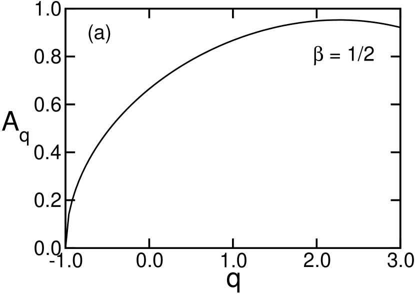
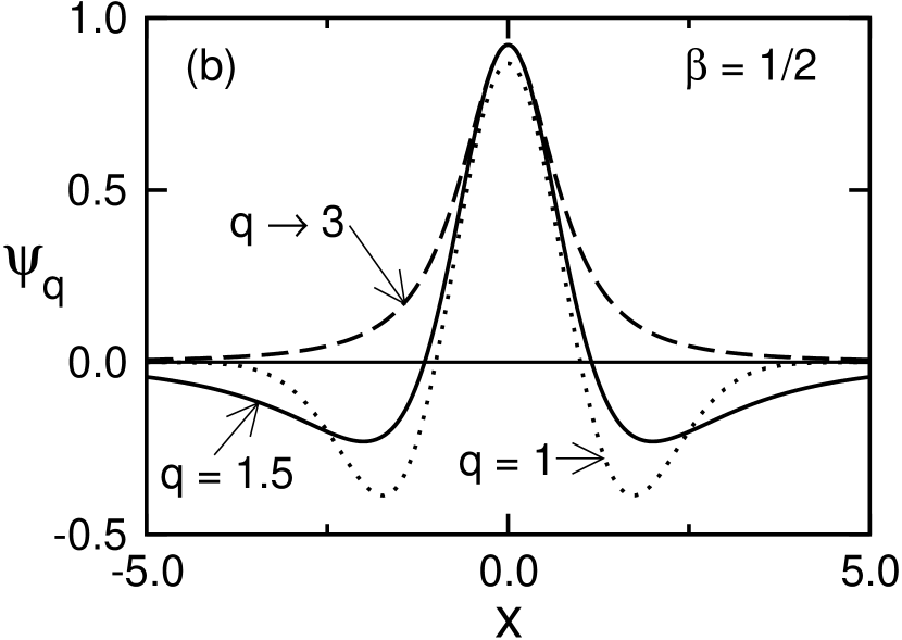
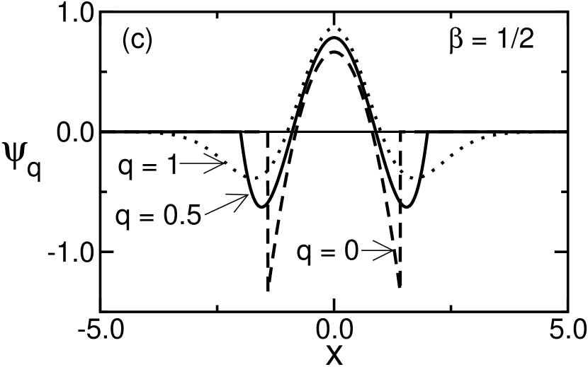
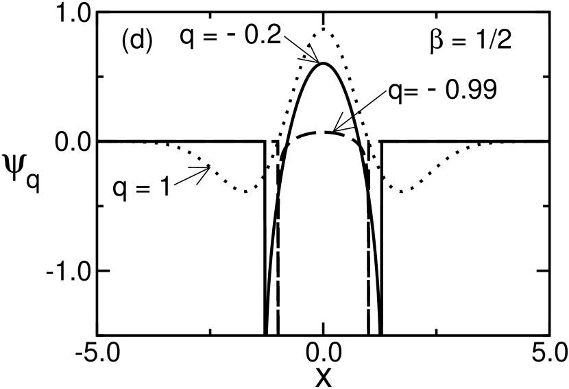
Figure 1: $q$-mexican hat with $\beta=1/2$. (a) Normalization constant $A_{q}$; (b) $\psi_{q}(x)$ for $1<q<3$; (c) $0<q<1$; (d) $-1<q<0$. The usual mexican hat ($q=1$) is represented by a dotted line, for comparison.

The function $\psi_{q}(x)$ satisfies the admissibility condition and consistently recovers the mexican hat, $\lim_{q\rightarrow 1}\psi_{q}(x)=\psi_{1}(x).$ The range of admissible values for $q$ $(-1<q<3)$ is divided in three regions. For $1<q<3$, $\psi_{q}(x)$ is infinitely supported and presents a power-law tail $\sim-1/|x|^{2/(q-1)}$, in marked contrast with the exponential tail of the original mexican hat. When $q<1$, a cut-off naturally appears at $|x_{c}|=[(1-q)\beta]^{-1/2}$. In the range $0<q<1$, $\psi_{q}(x_{c})=0$, and when $-1<q<0$, $\psi_{q}(x_{c})$ diverges. For $q\rightarrow-1$, $\psi_{q}(x)$ coincides with the abscissa axis, except at the cut-off positions, where it diverges. These features introduce significant differences from the original mexican hat wavelet. Figure 1 illustrates $\psi_{q}(x)$ with $\beta=1/2$.

The Fourier transform,

$${\cal F}\left[f(x);\,y\right]\equiv F(y)\equiv\frac{1}{\sqrt{2\pi}}\int_{-\infty}^{\infty}\mbox{e}^{ixy}\,f(x)\,\mbox{d}x,$$ (21)

of $\psi_{q}(x)$ may be found by considering (17), and taking into account the property of the Fourier transform of derivatives, ${\cal F}\left[f^{(n)};\,y\right]=(-iy)^{n}\,F(y),$ together with the Fourier transform of a $q$-Gaussian (see Equations 3.384 9 and 3.387 2 of [48]). We find for $1<q<3$,

$${\cal F}\left[\psi_{q}(x);\,y\right]=\frac{A_{q}}{(2-q)\beta}\frac{1}{\sqrt{2(q-1)\beta}\,\Gamma\left(\frac{2-q}{q-1}\right)}y^{2}\left[\frac{|y|}{2\,\sqrt{(q-1)\beta}}\right]^{\nu}$$

$$\times K_{\nu}\left(\frac{|y|}{\sqrt{(q-1)\beta}}\right),$$ (22)

and for $-1<q<1$,

$${\cal F}\left[\psi_{q}(x);\,y\right]=\frac{A_{q}}{2(2-q)\beta}\frac{\Gamma\left(\frac{2-q}{1-q}+1\right)}{\sqrt{2(1-q)\beta}}\;y^{2}\left[\frac{2\sqrt{(1-q)\beta}}{y}\right]^{-\nu}$$

$$\times J_{-\nu}\left(\frac{y}{\sqrt{(1-q)\beta}}\right),$$ (23)

with $\nu=\frac{2-q}{q-1}-\frac{1}{2}$. $J_{-\nu}$ is the Bessel functions of first kind and $K_{\nu}$ is the modified Bessel function of second kind.

It is possible to have variations of the $q$-mexican hat by using $\beta=\beta(q)$ (with $\beta(1)=\frac{1}{2}$), for instance, $\beta=1/(3-q)$.

3 Modulated $q$-Gaussian

Now we turn to the Morlet’s wavelet, or modulated Gaussian [49, 50, 51], a function associated with the birth of wavelet analysis [52, 53]. Within the context we are dealing with, we search for a wavelet that is a generalization of [40, 54]:

$$h(x)=\pi^{-1/4}\,(\mbox{e}^{-ikx}-\mbox{e}^{-k^{2}/2})\,\mbox{e}^{-x^{2}/2},$$ (24)

where $k=\pi(2/\ln 2)^{1/2}$. So we simply modulate the usual trigonometric functions ($\mbox{e}^{-ik_{q}x}$) with a $q$-Gaussian ($\mbox{e}_{q}^{-\beta x^{2}}$):

$$h_{q}(x)=B_{q}\,\left(\mbox{e}^{-ik_{q}x}-\Lambda_{q}(k_{q})\right)\,\mbox{e}_{q}^{-\beta x^{2}},\quad\infty<q<3.$$ (25)

The function $\Lambda_{q}(k_{q})$ is such that the admissibility condition, written in the domain of frequencies,

$${\cal F}[h_{q}(x);\,0]=0,$$ (26)

is satisfied. It means that

$$\Lambda_{q}(k_{q})\equiv\frac{{\cal F}\left[\mbox{e}^{-ik_{q}x}\,\mbox{e}_{q}^{-\beta x^{2}};\,0\right]}{{\cal F}\left[\mbox{e}_{q}^{-\beta x^{2}};\,0\right]}.$$ (27)

Taking into account the Fourier transform of a $q$-Gaussian (see Equations 3.384 9 and 3.387 2 of [48]), and ${\cal F}[\mbox{e}^{-ik_{q}x};\,y]=\sqrt{2\pi}\,\delta(y-k_{q})$, and also, from the convolution theorem (with the symmetric convention (21) we are adopting here),

$${\cal F}\left[f(x)\,g(x);\,y\right] = F(y)\ast G(y)$$ (28)

$$= \frac{1}{\sqrt{2\pi}}\int_{-\infty}^{\infty}F(y-\xi)\,G(\xi)\,\mbox{d}\xi,$$

we find for $q>1$,

$$\Lambda_{q}(k_{q})=\frac{2}{\Gamma\left(\frac{1}{q-1}-\frac{1}{2}\right)}\left(\frac{k_{q}}{2\,\sqrt{(q-1)\beta}}\right)^{\mu}K_{\mu}\left(\frac{k_{q}}{\sqrt{(q-1)\beta}}\right),$$ (29)

and for $q<1$,

$$\Lambda_{q}(k_{q})=\Gamma\left(\frac{1}{1-q}+\frac{3}{2}\right)\left(\frac{2\,\sqrt{(1-q)\beta}}{k_{q}}\right)^{-\mu}J_{-\mu}\left(\frac{k_{q}}{\sqrt{(1-q)\beta}}\right),$$ (30)

with $\mu=\frac{1}{q-1}-\frac{1}{2}$. We follow the same criterion adopted by [40] for the determination of the value of $k_{q}$: the ratio between the second highest and highest local maxima of $\mbox{Re }h_{q}$ is $\frac{1}{2}$. It results that

$$k_{q}=2\pi\sqrt{\frac{(q-1)\beta}{2^{q-1}-1}}\qquad(q\stackrel{{\scriptstyle\scriptscriptstyle>}}{{\scriptscriptstyle<}}1).$$ (31)

The normalization constant $B_{q}$ is given by

$$B_{q}=\left\{\begin{array}[]{lc}\left(\frac{\beta}{\pi}\right)^{1/4}\left[\frac{(q-1)^{1/2}\,\Gamma\left(\frac{2}{q-1}\right)}{\Gamma\left(\frac{2}{q-1}-\frac{1}{2}\right)}\right]^{1/2},&1<q<3,\\ \vskip 6.0pt plus 2.0pt minus 2.0pt\cr\left(\frac{\beta}{\pi}\right)^{1/4}\left[\frac{(1-q)^{1/2}\,\Gamma\left(\frac{2}{1-q}+\frac{3}{2}\right)}{\Gamma\left(\frac{2}{1-q}+1\right)}\right]^{1/2},&\qquad q<1.\end{array}\right.$$ (34)

($B_{q}$ is an approximation, as $B_{1}=\pi^{-1/4}$ of Equation (24) is also an approximation.) Figure 2 illustrates $\sqrt{2}\,\mbox{Re }h_{q}$ with $\beta(q)=1/(3-q)$. (The factor $\sqrt{2}$ is used to have the real part normalized.) We observe the long (power-law) tail for $1<q<3$, in marked contrast with the rapidly vanishing tail for $q=1$. The cut-off is present for $q<1$. In the case $q\rightarrow-\infty$, $h_{q}(x)$ reduces to a two-cycle function, the imaginary part of it is a variation of the one-cycle sine presented in [40].

4 $q$-Trigonometric wavelets

The $q$-exponential function (11), expanded to the imaginary (or, more generally, complex) domain by analytic continuation, leads to $q$-trigonometric functions [32]:

$$\cos_{q}x=\frac{\mbox{e}_{q}^{ix}+\mbox{e}_{q}^{-ix}}{2},\qquad\sin_{q}x=\frac{\mbox{e}_{q}^{ix}-\mbox{e}_{q}^{-ix}}{2i}.$$ (35)

The $q$-cosine and $q$-sine functions may be expressed as $\mbox{e}_{q}^{ix}=\rho_{q}(x)\,\mbox{e}^{i\varphi_{q}(x)}$ where

$$\rho_{q}^{2}(x)=\mbox{e}_{q}^{(1-q)x^{2}},\qquad\varphi_{q}(x)=\frac{\arctan_{1}[(1-q)x]}{1-q}.$$ (36)

We want to construct a wavelet based on such $q$-trigonometric functions. For this purpose, we recall that the derivative of a $q$-exponential may be expressed as

$$\frac{\mbox{d}\mbox{e}_{q}^{x}}{\mbox{d}x}=\mbox{e}_{2-1/q}^{qx}\,.$$ (37)

Once $\rho_{q>1}(x)\rightarrow 0$ for $|x|\rightarrow\infty$, the admissibility condition is satisfied for $1<q<2$. Renaming the parameter $q$, we define the following $q$-trigonometric wavelet:

$$\mbox{wt}_{q}(x)\equiv C_{q}\,\mbox{e}_{q}^{\frac{ix}{2-q}},\qquad 1<q<2.$$ (38)

The normalization constant is given by:

$$C_{q}=\sqrt{\frac{1}{2-q}}\,\frac{1}{\pi^{1/4}}\left[\frac{(q-1)\,\Gamma\left(\frac{1}{q-1}\right)}{\Gamma\left(\frac{1}{q-1}-\frac{1}{2}\right)}\right]^{1/2}.$$ (39)

For brevity of notation, we can write the real and imaginary parts of $\mbox{wt}_{q}(x)$ as

$$\mbox{wc}_{q}(x)\equiv\sqrt{2}\,\mbox{ Re }\mbox{wt}_{q}(x)=\sqrt{2}\,C_{q}\,\cos_{q}\left(\frac{x}{2-q}\right),$$ (40)

$$\mbox{ws}_{q}(x)\equiv\sqrt{2}\,\mbox{ Im }\mbox{wt}_{q}(x)=\sqrt{2}\,C_{q}\,\sin_{q}\left(\frac{x}{2-q}\right).$$ (41)

Some typical curves are shown in Figure 3 (for brevity, we only show the odd function $\mbox{ws}_{q}(x)$). Note that the number of oscillations decreases as $q$ goes from $1$ to $2$. The functions present infinite oscillations of vanishing amplitudes at $q\rightarrow 1$ ($C_{q\rightarrow 1}\rightarrow 0$). $\mbox{ws}_{q}(x)$ presents only one root, at $x_{0}=0$, for $\frac{3}{2}\leq q<2$, and $\mbox{wc}_{q}(x)$ presents only one pair of roots, at $x_{0}=\pm\,\frac{2-q}{q-1}\,\tan\left[(q-1)\frac{\pi}{2}\right],$ for $\frac{4}{3}\leq q<2$. As $q\rightarrow 2$, $C_{q}\rightarrow\infty$, and the wavelets become sharply localized (the roots of $\mbox{wc}_{q}(x)$ approaches $\pm\,2/\pi$). Let us also mention that the modulation of the functions is not Gaussian, but rather a power-law decay. But they are essentially different from the modulated $q$-Gaussian derived in the previous Section.

The Fourier transform of $\mbox{wc}_{q}(x)$ and $\mbox{ws}_{q}(x)$ are found with Equation (35) and (see Equations 3.382 6 and 3.382 7 of [48])

$${\cal F}\left[\mbox{e}_{q>1}^{iax};\,y\right]=\left\{\begin{array}[]{ll}0\;,&y>0,\\ \vskip 6.0pt plus 2.0pt minus 2.0pt\cr\displaystyle\frac{\sqrt{2\pi}\,(-y)^{\frac{1}{q-1}-1}\,\mbox{e}^{\frac{y}{(q-1)a}}}{[(q-1)a]^{\frac{1}{q-1}}\,\Gamma\left(\frac{1}{q-1}\right)},&y<0,\end{array}\right.$$ (44)

and

$${\cal F}\left[\mbox{e}_{q>1}^{-iax};\,y\right]=\left\{\begin{array}[]{ll}\displaystyle\frac{\sqrt{2\pi}\,y^{\frac{1}{q-1}-1}\,\mbox{e}^{\frac{-y}{(q-1)a}}}{[(q-1)a]^{\frac{1}{q-1}}\,\Gamma\left(\frac{1}{q-1}\right)},&y>0,\\ \vskip 6.0pt plus 2.0pt minus 2.0pt\cr 0\;,&y<0.\end{array}\right.$$ (47)

5 An Example

Wavelet transforms constitute a multi-purpose tool that rapidly met widespread applications in many areas of pure and applied sciences. To exemplary demonstrate the reliability of $q$-wavelets, we briefly present how they can be used to reproduce several properties of well known fractal sets.

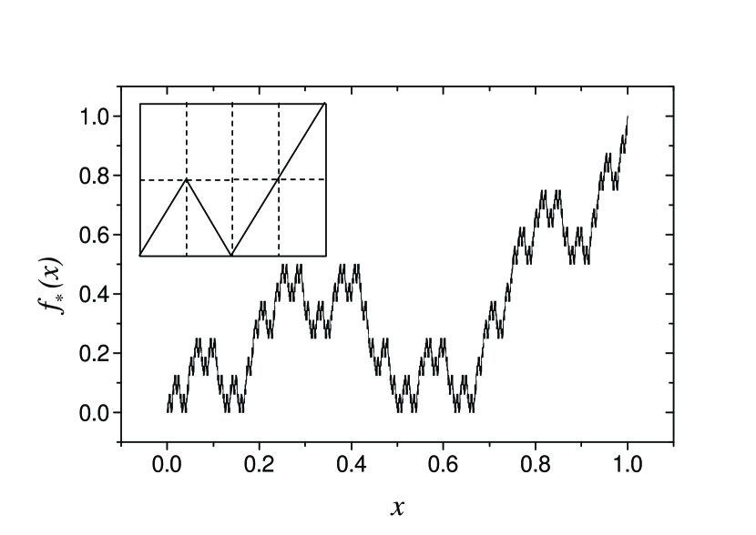
Figure 4: Self-affine monofractal profile. Inset: its generator.

Consider a self-affine profile $y=f_{*}(x)$ shown in Figure 4. Its construction starts with the generator shown in the Inset. The generator is recursively applied for each straight line segment. The self-affine fractal profile is obtained in the limit of infinite iterations.

The resulting figure after infinite generations has a local fractal dimension $D=2-\alpha,$ where $\alpha=\ln B_{y}/\ln B_{x}=0.5$ is the roughness exponent, and $B_{x}$ and $B_{y}$ are the scaling factors along the $x$ and $y$ axis respectively. To analyze the scaling properties of $f(x)$ around an arbitrary point $x_{0},$ we shift the origin and define

$$f_{x_{0}}(x)=f(x_{0}+x)-f(x_{0})\approx Ax^{\alpha(x_{0})}$$ (48)

where $\alpha(x_{0}),$ the Holder (or singularity) exponent of $f_{x_{0}}(x),$ indicates how this function vanishes (or diverges) at $x=x_{0}.$

Using a general wavelet transform of $f_{x_{0}}(x),$ it is straightforward to show that the Holder exponent follows immediately from the wavelet transform as

$$T_{g}(a,b)\;f_{x_{0}}(x)\sim a^{\alpha(x_{0})}.$$ (49)

Figure 5 shows how the $q$-wavelet transform (Equation (49)) behaves for two points along the profile for some values of $q.$ The curves clearly indicates that the value $\alpha=0.5$ is accurately reproduced. We observe that the results for $q>1$ show small irregularities. This is due to the fact that, as $\mbox{e}_{q}^{-x}$ decays only as a power-law when $x\rightarrow\infty$, the numerical integration in (49) must be performed over a wider interval than for $q\leq 1.$ In order to make evident this effect, we have performed all integrals over a fixed integration interval. On the other hand, results for $q<1$ show good convergence, as the function naturally presents a cutoff. Oscillations in the curves are typical for this kind of analysis, as shown in the same figure for the usual mexican hat ($q=1$).

Results for a more complex situation can be explored if we consider a multifractal set. It is generated along a similar way used to obtain the first set, where we choose two different scaling factors for the first and second half of the profile in each generation of its construction. The plots for different values of $x_{0}$ have different slopes (Figure 6), indicating that many scaling laws and fractal dimensions are found in the resulting profile.

$q$-Wavelets also prove to be a reliable tool to analyze this much more complex situation that requires a multi-fractal formalism. This amounts to evaluate the generalized fractal dimensions $D_{Q},$ or its Legendre transformed singularity spectrum $f(\alpha)=\tau(q)-\alpha Q$, where $\alpha$ represents the Holder exponent. This analysis proceeds within the so-called Wavelet Transform Modulus-Maxima Method (WTMMM), that has been developed in recent years. We will not show the details that can be found, e.g., in [55].

Figure 7 shows the $f(\alpha)$ spectra, for different values of $q$, corresponding to the multifractal profile. The graphs indicate that the spectra produced by $q$-wavelets, with $q<1$, are comparable to the one obtained by the usual $q=1$ mexican hat. As we fixed the integration interval for all values of $q,$ we observe major differences in the spectra for values $q>1.$ This limitation to its practical use is expressed by larger numerical effort to compute the integrals in the wavelet transforms with the same accuracy for values of $q\leq 1$.

6 Final Remarks

The functions here introduced generalize widely used mother wavelet functions by means of a single parameter. The $q$-wavelets present significant different behaviours, when compared with the original $q=1$ cases. The fingerprints of the generalized $q$-wavelets are the power-law decay $(q>1)$, and the cut-off $(q<1)$. The generalization was inspired in the nonextensive statistical mechanics and the $q$-exponential that emerges from it. Within this formalism, the entropic index $q$ measures departures from the usual Boltzmann-Gibbs behaviour. There is a number of possible origins for such departures, like slow (power-law) mixing, long-range (spatial) interactions, long-term (temporal) memory or fractal nature of the phase space. When dealing with signals which exhibit some of these features, one can hopefully take advantage of the index $q$ to tune the wavelet to the signal, as it is here briefly exemplified for the $q$-mexican hat. Other wavelets, as well as scaling functions, may be generalized along the lines here introduced, for instance, the Meyer wavelet or the sinc function.

7 Acknowledgments

We thank C Rodrigues Neto for his collaboration at the early stages of this project, and E K Lenzi for useful remarks. This work is partially supported by PRONEX/MCT, CNPq, CAPES and FAPERJ (Brazilian agencies).

Figure 2: Normalized real part of the $q$-modulated Gaussian ($h_{q}^{R}(x)\equiv\sqrt{2}\,\mbox{Re }h_{q}$). (a) $q=1$ (usual case); (b) $q=2$; (c) $q\to-\infty$ (illustrated with $q=-100$). Note that abscissa scale in (c) is different from the others.

Figure 3: $\mbox{ws}_{q}(x)$ vs. $x$. (a) $q=1.01$; (b) $q=1.1$ (solid) and $q=1.99$ (dashed).

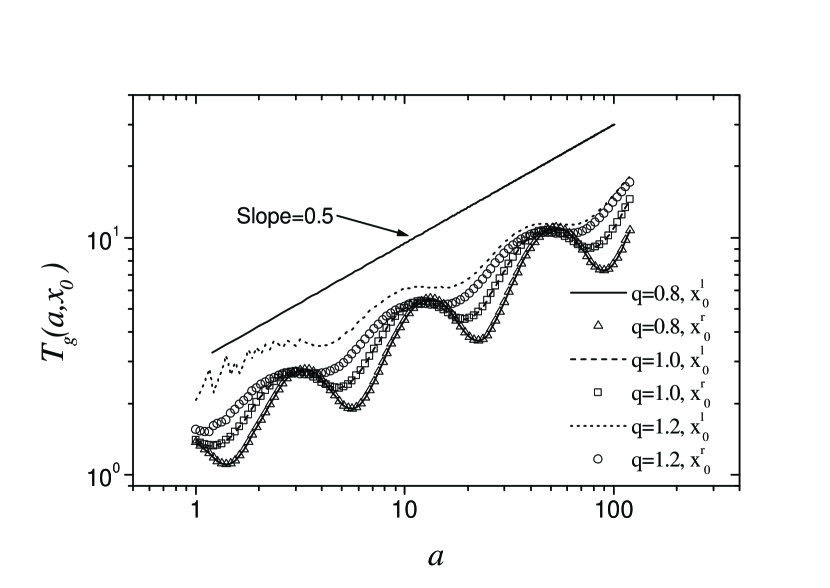
Figure 5: Wavelet transform (Equation (49)) with two different values of $b$: $x^{l}_{0}=0.25$ and $x^{r}_{0}=0.50$. Note that the curves for the same values of $q$ coincide, as it should be for a monofractal.

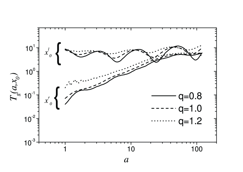
Figure 6: Wavelet transform (Equation (49)) with two different values of $b$: $x^{l}_{0}=0.25$ (upper curves) and $x^{r}_{0}=0.75$ (lower curves). The slopes are clearly different, as a signature of the multifractal nature.

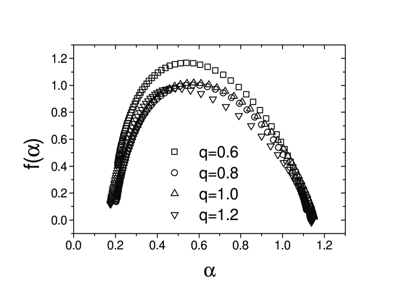
Figure 7: $f(\alpha)$ spectra for the multifractal profile. For $q=0.8$ results are very similar to those with $q=1$. $q=0.6$ yields spurious results.

References

- [1] Kreyszig E 1993 Advanced Engineering Mathematics (New York: John Wiley & Sons, 7th ed.)
- [2] Ray Wylie C and Barrett L C 1985 Advanced Engineering Mathematics (Singapore: McGraw-Hill Book Company, 5th ed.)
- [3] Gabor D 1946 J. Inst. Elect. Eng. (London) 93 no. III 429–57
- [4] Kaiser G 1994 A Friendly Guide to Wavelets (Boston: Birkhäuser)
- [5] Fourier J 1822 Théorie Analytique de la Chaleur in Darboux G 1888 Œuvres de Fourier Tome Premiére (Paris: Gauthier-Villars et Fils)
- [6] Tsallis C 1988 J. Stat. Phys. 52 479–87
- [7] Curado E M F and Tsallis C 1991 J. Phys. A 24 L69; Corrigenda: 1991 24 3187 and 1992 25 1019
- [8] Abe S and Okamoto Y (eds.) 2001 Nonextensive Statistical Mechanics and its Applications, Series Lecture Notes in Physics (Berlin: Springer-Verlag)
- [9] Gell-Mann M and Tsallis C 2004 (eds.) Nonextensive Entropy — Interdisciplinary Applications (New York: Oxford University Press)
- [10] Alemany P A and Zanette D H 1994 Phys. Rev. E 49 R956–8
- [11] Zanette D H and Alemany P A 1995 Phys. Rev. Lett. 75 366–9
- [12] Tsallis C, de Souza A M C and Maynard R 1995 Derivation of Lévy-type anomalous superdiffusion from generalized statistical mechanics, in Shlesinger M F, Zaslavsky G M and Frisch U (eds.) Lévy flights and related topics in Physics 269–89 (Berlin: Springer)
- [13] Zanette D H 1999 Braz. J. Phys. 29 108–24
- [14] Wilk G and Włodarczyk Z 2000 Phys. Rev. Lett. 84 2770–3
- [15] Tsallis C, Levy S V F, de Souza A M C and Maynard R 1996 Phys. Rev. Lett. 75 3589–93; 1996 77 5442 (erratum)
- [16] Prato D and Tsallis C 1999 Phys. Rev. E 60 2398–401
- [17] Plastino A R and Plastino A 1993 Phys. Lett. A 174 384–6
- [18] Hamity V H and Barraco D E 1996 Phys. Rev. Lett. 76 4664–6
- [19] Boghosian B M 1996 Phys. Rev. E 53 4754–63
- [20] Anteneodo C and Tsallis C 1997 J. Mol. Liq. 71 255–67
- [21] Boghosian B M 1999 Braz. J. Phys. 29 91–107
- [22] Arimitsu T and Arimitsu N 2000 Phys. Rev. E 61 3237–40
- [23] Arimitsu T and Arimitsu N 2000 J. Phys. A: Math. Gen. 33 L235–41
- [24] Beck C 2000 Physica A 277 115–23
- [25] Beck C, Lewis G S and Swinney H L 2001 Phys. Rev. E 63 035303(R)
- [26] Tsallis C, Anjos J C and Borges E P Phys. Lett. A 310 (5-6) 372–76
- [27] Tsallis C and Borges E P 2003 Nonextensive statistical mechanics — Applications to nuclear and high energy physics, in Antoniou N G, Diakonos F K and Ktorides C N (eds.) Proc. 10th International Workshop on Multiparticle Production — Correlations and Fluctuations in QCD 326–43 (Singapore: World Scientific)
- [28] http://tsallis.cat.cbpf.br/biblio.htm
- [29] Tsallis C, Mendes R S and Plastino A R 1998 Physica A 261 534–54
- [30] Beck C and Schlögl F 1995 Thermodynamics of chaotic systems, (Cambridge: Cambridge University Press)
- [31] Tsallis C 1994 Quimica Nova 17 468–71
- [32] Borges E P 1998 J. Phys. A: Math. Gen. 31 5281–88
- [33] dos Santos R J V 1997 J. Math. Phys. 38 4104–07
- [34] Kassel C 1995 Quantum Groups (New York: Springer Verlag)
- [35] Gamero L G, Plastino A and Torres M E 1997 Physica A 246 487–509
- [36] Capurro A, Diambra L, Lorenzo D, Macadar O, Martin M T, Mostaccio C, Plastino A, Rofman E, Torres M E and Velluti J 1998 Physica A 257 149–55
- [37] Capurro A, Diambra L, Lorenzo D, Macadar O, Martin M T, Mostaccio C, Plastino A, Perez J, Rofman E, Torres M E and Velluti J 1999 Physica A 265 235–54
- [38] Martin M T, Plastino A R and Plastino A 2000 Physica A 275 262–71
- [39] Tong S, Bezerianos A, Malhotra A, Zhu Y and Thakor N 2003 Phys. Lett. A 314 354–61
- [40] Daubechies I 1990 IEEE Trans. Inform. Theory 36 961–1005
- [41] Daubechies I 1992 Ten Lectures on Wavelets CBMS-NSF Regional Conference Series in Applied Mathematics, Vol. 61, (Philadelphia: Society for Industrial and Applied Mathematics, SIAM)
- [42] Hernández E and Weiss G 1996 A First Course on Wavelets (Boca Raton: CRC Press)
- [43] Tsallis C 2001 Nonextensive statistical mechanics and thermodynamics: Historical back-ground and present status, in [8], p. 3
- [44] Borges E P 2004 Physica A 340 95–101
-
[45]
Suyari H and Tsukada M 2004
Law of Error in Tsallis Statistics,
e-print
[http://arXiv.org/cond-mat/0401540] -
[46]
Suyari H 2004
Mathematical structure derived from the -multinomial coefficient
in Tsallis statistics,
e-print
[http://arXiv.org/cond-mat/0401546] -
[47]
Suyari H 2004
-Stirling’s formula in Tsallis statistics,
e-print
[http://arXiv.org/cond-mat/0401541] - [48] Gradshteyn I S and Ryzhik I M 1994 Table of Integrals, Series, and Products A. Jeffrey (ed.) (San Diego: Academic Press, 5th ed.)
- [49] Morlet J, Arens G, Fourgeau I and Giard D 1982 Geophys. 47 203–36
- [50] Grossmann A and Morlet J 1984 SIAM J. Math. Anal. 15 723–36
- [51] Grossmann A and Morlet J 1985 Decomposition of functions into wavelets of constant shape and related transforms, in Streit L (ed.) Mathematics and Physics, Lectures on Recent Results (Singapore: World Scientific Publishing)
- [52] Temme N M 1993 Wavelets: First Steps, in Koornwinder T K (ed.) Wavelets: An Elementary Treatment of Theory and Applications 1–12 (Singapore: World Scientific)
- [53] Meyer Y 1990 Ondelettes (Paris: Hermann, Éditeurs des sciences et des arts)
- [54] Holschneider M 1995 Wavelets, An Analysis Tool, (Oxford: Clarendon Press)
- [55] Muzy J F, Bacry E and Arneodo A 1994 Int. J. Bif. Chaos 4 245–302