Under-knotted and over-knotted polymers: compact self-avoiding loops

Abstract

We present a computer simulation study of the compact self-avoiding loops as regards their length and topological state. We use a Hamiltonian closed path on the cubic-shaped segment of a $3D$ cubic lattice as a model of a compact polymer. The importance of ergodic sampling of all loops is emphasized. We first look at the effect of global topological constraint on the local fractal geometry of a typical loop. We find that even short pieces of a compact trivial knot, or some other under-knotted loop, are somewhat crumpled compared to topology-blind average over all loops. We further attempt to examine whether knots are localized or de-localized along the chain when chain is compact. For this, we perform computational decimation and chain-coarsening, and look at the ”renormalization trajectories” in the space of knots frequencies. Although not completely conclusive, our results are not inconsistent with the idea that knots become de-localized when the polymer is compact.

I Introduction

I.1 Goal and plan of this work

In the preceding articlepreceding , we have discussed the idea of two distinct scaling regimes for the closed polymer loop, we called them the over-knotted and under-knotted regimes. They are different in terms of the relation between a given loop with quenched topology and the imaginary loop with annealed topology, the latter being able to freely cross itself. Loosely speaking, for the over-knotted loop, topological constraints prevent the loop from untying its knots, from simplifying the knots or reducing their numbers. For the under-knotted loops, the effect is the opposite, for the topological constraints prevent the loop in this case from forming more knots. We argued that under-knotted loops tend to swell beyond the size of the phantom loop, while over-knotted loops tend to be more compact.

In the present article, we wish to extend this qualitative idea for another context, namely, for the polymers which are compressed by either external pressure or by some sort of poor solvent effect, the latter being equivalent to somewhat sticky segments. This problem is highly relevant, because most biopolymers are compact in their native conditions. DNA, for instance, is frequently so long that it would not fit inside the cell if allowed to fluctuate freely.

We shall argue first of all that the natural zeroth approximation for such a problem of compact loops can be formulated in terms of Hamiltonian paths on cubic shaped piece of a regular lattice in space. In the following sections we shall briefly describe our approach to computational generation of the maximally compact loops on a cubic lattice. This approach was formulated in the work1 . Next we present probabilities of obtaining unknotted configurations, as well as probabilities of obtaining a few simple knots. We also present measurements of the average spatial extent of segments or sub-chains of compact conformations and analyze how these measurements depend on the topology or knot-type of the conformations.

Through the latter measurements, we address the question how global knot topology of a large loop affects local fractal geometry of typical trajectories. An exciting general problem here, which we think is an important challenge for the future, is to which extent looking at local geometry of chains allows guessing of their global topology.

We should point out that compact loops very rapidly become under-knotted with increasing loop length with fixed knot state, because the ensemble of all loops (or, equivalently, the ensemble of states of a phantom loop) is dominated by very complex knots when loop is compact. Thus, what we study is the local fractal geometry of under-knotted loops. This already suggests the result, which we shall explain in more depth later, that the pieces of under-knotted compact loop are locally somewhat crumpled compared to their phantom counterparts.

There is also an interesting question of whether the knots tend to be spread out or confined to a small portion of the polymer. Previous theoretical and computational workknot_inflation ; 6 ; localization_2 ; localization_3 have shown that knot-determining domains for non-compact loops are usually rather tight. For instance, the preferred size of the trefoil-determining portions of knotted polymer chains corresponds to just seven freely jointed segments6 . In that work, the knotted domain is identified by looking for the minimal number of contiguous segments belonging to the circular chain such that, upon closure with an external planar loop, the new knot formed is of the same type as the original knot.

One possible interpretation would be that knot localization is the property of all under-knotted loops. From that point of view, it is interesting to look at knot localization in compact loops, as they are heavily under-knotted. So far, we are aware of only one numerical work7 addressing this issue for prime flat knots in a model of self-attracting polymers with excluded volume. Here, when we say ”flat” we mean that the polymer is strongly adsorbed onto a flat surface, or confined in a thin planar slit. It was found in7 that these flat knots are localized in the high temperature swollen regime (consistent with theoretical predictionlocalization_3 ), but become delocalized in the low temperature, collapsed globular phase. For three-dimensional polymers, the conjecture is that there is also a similar delocalization transition, i.e. the knots are delocalized for compact circular chains. We shall attempt to address this issue of knot (de)localization for compact circular chains.

I.2 Why lattice model is natural for our purposes

In order to address knots in densely compressed loops it is very important to realize the role of excluded volume, or self-avoidance. Physically, this is the short range repulsive forces which always exist and which prevent pieces of polymer from penetrating each other. Mathematically, self-avoidance condition specifies the ensemble of allowed loop shapes. When loop is not geometrically restricted, as it was examined in the preceding articlepreceding , these excluded volume constraints are often irrelevant. That is why, for the purposes of the preceding paperpreceding , we argued it possible to view polymer loop as just a closed continuous mathematical line, with no thickness. For such object, the measure of trajectories with self-overlaps is exactly zero, and so the probabilities of all distinct knot topologies sum up to unity. For the compact loop, such model becomes meaningless, because the limit of zero thickness is singular for loops restricted to within certain volume. The meaningful model in this case implies that the density is maintained constant all across the allowed volume, which exactly corresponds to imposing the self-avoidance condition along with the volume restriction.

The simple model capturing self-avoidance condition is a polymer presented as a path on the regular lattice in space, such as cubic lattice. Knots in lattice polymers were examined in a number of works. In particular, it was proven in the workstheorem1 ; theorem2 that the probability to obtain a trivial knot upon random generation of the lattice polygon of $N$ segments decays exponentially in $N$. We should emphasize that this is different from the problem addressed in our preceding articlepreceding , because we looked at the loops with no volume exclusion, while every lattice model suitable for the study of knots and thus excluding self-intersections involves automatically some excluded volume. Unlike geometrically unrestricted loops, for the problem of compact loops excluded volume is what we must take into account, and, therefore, lattice path is now a natural model to look at.

In order to make it compact, we now consider a segment of cubic lattice, say, a cube of the some size $m\times m\times m$, and consider a path of $N=m^{3}$ self-avoiding steps confined in this cube. Obviously, this is a Hamiltonian path. For the purposes of modelling the closed polymers, we shall consider here Hamiltonian closed paths, or Hamiltonian loops.

II Brief overview of our recent results1

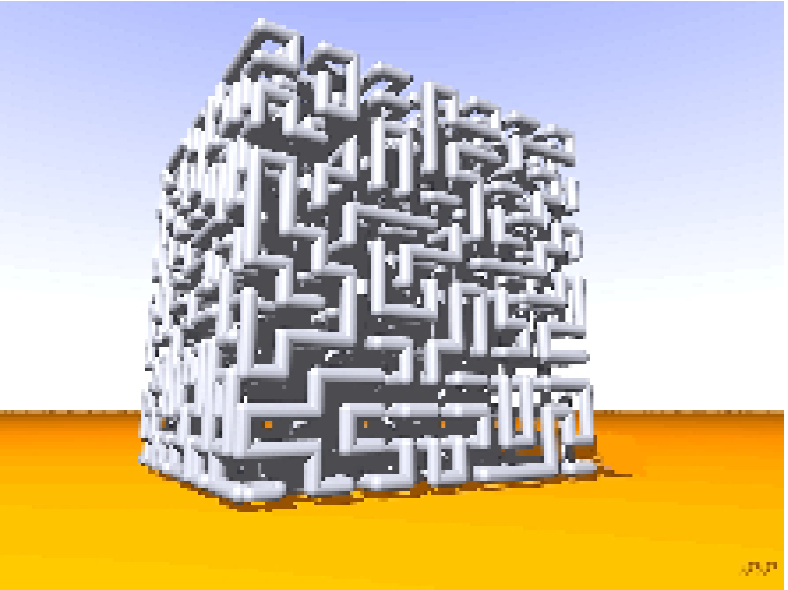
Figure 1: A $14\times 14\times 14$ compact conformation on a lattice rendered by Professor Piotr Pieranski. The three knot invariants calculated for this conformation correspond to a trivial knot. Using a knot-tightening algorithm called Shrink On No OverlapsSONO (SONO), Professor Pieranski verified that the conformation is indeed unknotted by reducing the conformation into a small circular loop.

II.1 Generation of compact loops

The method we used to generate compact conformations on a lattice is described in Ref. 1 . It is based on a combinatorial algorithm by Ramakrishnan et al2 . The method essentially works by placing links randomly on the lattice, avoiding sub-cycles and dead ends, until a single loop fills the desired cubic lattice dimensions. For closed loops (Hamiltonian walks), conformation dimensions can only be even ($2\times 2\times 2$, $4\times 4\times 4$, etc.). Note that the method does not use a conventional process in which a single connected chain is grown to the desired size, because the rejection rate of any such process for compact chains rapidly becomes catastrophic even at modest chain length. Figure 1 illustrates an example of a $14\times 14\times 14$ conformation. Although our method is not free of biases and is not perfect, it is a significant improvement over the original algorithm by Ramakrishnan et al.

II.2 Topology

We identified the knot-type (${\cal K}$) of a conformation by calculating the following three knot invariants: the Alexander polynomial evaluated at $t=-1$ ($\Delta(-1)_{\cal K}$), the Vassiliev invariant of degree two ($v_{2}({\cal K})$) and the Vassiliev invariant of degree three ($v_{3}({\cal K})$). For example, the knot invariants for an unknot or trivial knot (${\cal K}\equiv 0_{1}$) are $|\Delta(-1)_{0_{1}}|=1,v_{2}(0_{1})=0,v_{3}(0_{1})=0$. Although, it is possible for two distinct knots to have the same set of knot invariants, we expect the false identification of knots to be rare. For instance, the set of three knot invariants are distinct from those of (prime) knots with 10 crossings or fewer (249 knots in all) in their projection.

Using these knot invariants to classify the conformations, we collected data for the frequency of occurrence of the trivial knot and the first few simple knots (Figure 2). Computational data on trivial knot probability are customarily fit to exponential, our last three data points giving $\sim\exp(-N/196)$.

An exponential fit should not be surprising, as the total number of conformations of length $N$ grows exponentially with $N$. The estimate of total number of compact conformations can be read out of the Floryfloryfirstbook theory of polymer melts. On the cubic lattice, and in accord with simulationsEnumeration , the number of compact conformations is $\sim\exp(sN)$, where $s\approx 0.62$. From that point of view, the above mentioned result of trivial knot probability fitting to $\sim\exp(-N/196)$ implies that topologically restricting polymer to have the topology of a trivial knot only reduces entropy per segment by about $1/196\approx 0.005$, which is a relatively insignificant amount compared to the entropy $s\approx 0.62$ itself. By contrast, to obtain an estimate from the other end, we can consider so-called crumpled conformations, similar to Peano curves. On the lattice, in the $2^{k}\times 2^{k}\times 2^{k}$ cube, they can be defined in the following way: the $2^{k}\times 2^{k}\times 2^{k}$ cube can be viewed as 8 smaller cubes $2^{k-1}\times 2^{k-1}\times 2^{k-1}$ each, and each smaller-subcube can be further divided in a similar way, etc, down to the smallest $2\times 2\times 2$ cubes. We define the trajectory to be crumpled if it visits all the vertices within given subcube before entering next subcube of the same level. It is easy to prove that crumpled conformations are trivial knots. The exact recurrence relation can be writtenmy_unpublished_result for the total number of crumpled conformations for the polymer of $N=8^{k}$ monomers, it yields the number of conformations about $\sim\exp(s^{\prime}N)$, with $s^{\prime}\approx 0.30$. Thus, there remains a huge room for speculation regarding the asymptotic value of trivial compact knot probability at $N\to\infty$. Strictly speaking, we cannot claim it is $196$ or close, we can only claim it is not larger than this quantity.

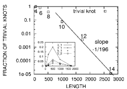
Figure 2: Trivial knot probabilities for compact conformations of size $4\times 4\times 4$ to $14\times 14\times 14$. Inset shows the probabilities of the non-trivial knots $3_{1}$ (trefoil), $4_{1}$ (figure-eight), $5_{1}$ (star), $5_{2}$.

The inset in figure 2 shows the probabilities of some non-trivial knots. The existence of a maximum is easily explained qualitatively as follows. When $N$ is small, the loop might be too short for a given knot, i.e. there is not enough ”room” for the knot to exist. It is clear in the lattice model that there is a finite number of segments required to form any given knot, e.g. $N=24$ for a trefoil3 . At the other extreme, when $N$ is large, there are many other knots ”competing” for formation. The number of complex knots increases with $N$, yielding a decaying probability to locate any given knot.

We also addressed the question of the spatial extent of segments of compact conformations. In particular, we were interested in determining if the segments of knotted conformations are more stretched-out or more compact compared to segments of unknotted conformations. (Note that even though the entire conformation is maximally compact, a connected piece of it need not be.) To this end, we collected conformations of length $N$ containing a particular knot and measured the mean-square end-to-end distances for segments or sub-chains of length up to $N^{2/3}$. We found that segments of knotted conformations are consistently more spread-out on average compared to segments of unknotted conformations. Figure 3 illustrates these results by plotting the ratios of mean-square end-to-end of segments of trefoil and figure-eight knotted conformations to unknotted conformations.

Figure 3: Mean square end-to-end of segments (sub-chains) of trefoil and figure-eight knotted conformations relative to that of trivially knotted conformations ($4\times 4\times 4,6\times 6\times 6,8\times 8\times 8$). Pieces of knots are more extended compared to pieces of unknots.

Figure 4: Mean square end-to-end of segments (sub-chains) of trefoil and figure-eight knotted conformations relative to that of the entire sample (”All”). Pieces of conformations that are over-knotted are more extended; Pieces of conformations that are under-knotted are more compact.

In figure 4, instead of taking the ratio over trivial knots, we took the ratio over all conformations in the sample regardless of topology. Although figure 4 seems hardly different from figure 3, much of the points for the $8\times 8\times 8$ trefoils and figure-eights in figure 4 correspond to ratios less than unity. This means the trefoil and figure-eight knotted conformations begin to be more compact than typical conformations for size $8\times 8\times 8$, i.e. these knots cross over from their over-knotted to their under-knotted regimes. In fact, for $8\times 8\times 8$, the percentage of trivial, trefoil and figure-eight knots in a fairly generated sample of conformations are 40%, 20% and 6.7% respectively. The rest of the more complex knots pull the average mean square end-to-end to values larger compared to those of trivial, trefoil and figure-eight knots. For smaller conformations of size $4\times 4\times 4$ and $6\times 6\times 6$, the topology is dominated by trivial knots.

III Testing knot localization hypothesis by renormalization

In this section we attempt to address the issue of knot localization for cicular chains using an idea inspired by field theory and polymer physics called renormalization or decimation4 . The idea is to group the $N$ segments of our original circular chain into $N/g$ blocks or blobs of $g$ units each. A new circular chain is formed by connecting the centers of mass of the blobs.

Our ”renormalization” procedure works as follows. Starting from a batch of chains of length $N$ with a given knot population distribution, we renormalize each chain to obtain a new batch of shorter chains of length $N_{1}=N/g$. We then compute the probabilities to obtain various knots for the new batch of renormalized or decimated chains and compare that to the knot probabilities of the original batch. If the knots are localized, we expect a renormalization step using a ”small” value of $g$ to obliterate or ”wash out” any memory of the original knot state. In other words, we expect a chain containing a localized knot and a chain containing no knots (or a localized knot of another type) to resemble each other after renormalization, with the value of $g$ giving an idea of the size of the knotted domain. For example, a trefoil knot formed by six straight links (sticks) of equal length will get totally unknotted after grouping consecutive units into pairs ($g=2$) to yield a chain containing just three (renormalized) units.

It is customary to present the results of a renormalization procedure by constructing a trajectory. In our case, the axes of the space in which the trajectory is plotted correspond to knot probabilities. Since the number of distinct knots is infinite, the dimension of this space is also infinite. To make the presentation more manageable, we plot the trajectory in a plane with one axis corresponding to the probability of trivial knots and the other axis corresponding to the probability of trefoil knots (Figure 5). In this plane, the important regions are marked. The point $(1,0)$ at the lower right hand corner of figure 5 corresponds to all knots being trivial, while the point $(0,1)$ at the upper left hand corner corresponds to pure trefoil knots. The line connecting these two points going diagonally corresponds to a sample containing either trivial and trefoil but no other knots. The region above this line, marked ”FORBIDDEN”, never gets visited by a trajectory by virtue of probabilities always summing to $1$. The region below this line corresponds to a sample containing more complex knots as well as trivial and trefoil knots. By plotting the knot population in each step (labeled by $g$) of the renormalization procedure, one gets a picture of the evolution of knot complexity. After a sufficient number of iterations or for large enough $g$, all trajectories should terminate at the point $(1,0)$ corresponding to completely unknotted chains.

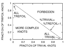
Figure 5: The space in which the trajectories are plotted. One can also consider it as a two dimensional slice of the infinite dimensional space of knot probabilities.

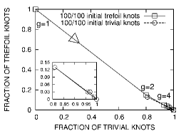
Figure 6: Knot renormalization trajectories for initial non-compact loops of length $N=384$. Inset shows the trajectory only for initial unknotted loops. (Initial trefoil knots - squares, initial trivial knots - circles).

We first tested this procedure by examining non-compact circular loops of length $N=384$, using an algorithm5 also described in a preceding article. We generated a batch of $100$ loops with trefoil knots and another batch of $100$ unknotted loops or trivial knots. The loops in each batch were renormalized into blobs of size $g=2,4,8,16,32,64$ units and the fraction of trefoils and trivial knots were computed for each $g$. When the probabilities for these knots are plotted against each other, one obtains figure 6.

In figure 6, the trajectory for the $100$ trefoils (squares) starts at the top of the vertical axis while the trajectory for the $100$ trivial knots (circles) starts at the extreme right along the horizontal axis. The trajectory of the initial trefoils takes an almost straight path down towards the unknotted region (indicated by the arrow), implying that the tendency to unknot is overwhelming (although a few non-trivial and non-trefoil knots were produced). The trajectory for the initial trivial knots first takes a short step away from the starting point (circle, $g=2$), meaning some knots predominantly trefoil are produced, then heads back towards the starting point.

The two trajectories first meet at $g=2$, when the chains become roughly indistinguishable topologically. The fraction of trivial knots at this point is $80\%$, which is significantly larger than the probability of getting a trivial knot from a random sample of loops with number of segments given by $N_{1}=N/g=384/2=192$. For $N_{0}=241$, the empirical unknotting probability5 is given by $w_{\rm triv}=\exp(-N_{1}/N_{0})=45\%$. These results seem to be consistent with the picture of a localized trefoil knot, using up just a few segments (6 or 7) of the entire chain.

The renormalization procedure outlined above was also applied to compact conformations on a cubic lattice of dimensions $8\times 8\times 8$ and $12\times 12\times 12$ (figures 7 and 8). Figure 7 illustrates the trajectories for initial $8\times 8\times 8$ compact conformations of $100$ trefoils and $100$ trivial knots. The trajectory of initial trefoils takes a downward path slightly skewed towards the origin. The trajectory of initial trivial knots makes a short excursion towards the origin then turns around and goes back to its starting point. The two trajectories seem to meet at about $g=16$. The interpretation of a localized or delocalized knot is not straightforward, since on a cubic lattice, the minimum number of segments needed to form a trefoil is $24$ instead of $6$.

The trajectories deviate significantly from the diagonal, manifesting the fact that many more complex knots are formed as a result of the renormalization procedure. This result is not surprising, as the distance between renormalized segments actually become smaller than the lattice constant of the original cubic lattice. In fact, renormalized segments may even overlap, after say $g=4$, due to congruences arising from the integral coordinate positions of the original chain units.

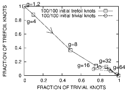
Figure 7: Knot renormalization trajectories for initial $8\times 8\times 8$ compact conformations. (Initial trefoil knots - squares, initial trivial knots - circles).

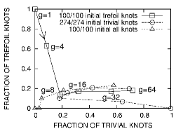
Figure 8: Knot renormalization trajectories for initial $12\times 12\times 12$ compact conformations. (Initial trefoil knots - squares, initial trivial knots - circles, initial ”all” knots - triangles).

Figure 8 illustrates the trajectories for initial $12\times 12\times 12$ compact conformations with $g=4,8,16,32,64$. Aside from batches of 100 trefoils and 274 trivial knots, we also added a batch of 100 conformations (triangles) regardless of topology, representing typical compact conformations for this size. In this ”all” knots batch, the probability for either a trivial knot or trefoil knot is about $2$ in $500$ (its starting point is thus located at the origin). In this regime, trivial knots and trefoil knots are overwhelmingly under-knotted. It can be seen from the trajectory of ”all” knots that the memory of the initial knot state does persist longer the more complex the initial knotted state. This result is also complemented by the behaviour of the trajectories of initial trefoils and trivial knots, which come close to the origin at $g=8$.

IV Conclusion

To conclude, we have examined the simple lattice model of compact polymer loops. To generate such loops computationally, we have employed what we believe is the least biased algorithm currently available1 . We first confirmed that the probability to realize a trivial knot is dramatically suppressed in compact loops compared to their volume-unrestricted counterparts. We sampled compact loops of up to $N=14^{3}=2744$ segments, and our data fit $\sim\exp(-N/N_{0})$ with $N_{0}\approx 196$. We emphasize that it remains unclear whether we have already reached the true $N\to\infty$ asymptotics, or in fact $N_{0}$ is smaller than our observed value of $196$. When we looked at the end-to-end distance of the small pieces of polymer, with some $g$ segments, $g\ll N^{2/3}$, we found that their end-to-end distances are smaller when the loop as a whole is a trivial knot, or, in general, when it is under-knotted, compared to the average over all loops or compared to complex knots or over-knotted loops. In principle, this allows for the possibility to make at least a probabilistic judgment of the global loop topology by observing its local fractal geometry. This is also consistent, at least qualitatively, with our findings in the preceding paperpreceding that confinement entropy grows with decreasing size much sharper for the topologically constrained loops such as trivial knots compared at the topology-blind average over all loops. We presented also first attempts to address knot de-localization in the collapsed polymers by looking at the renormalization trajectories in the space of knots frequencies. We think that our results open prospects for deeper understanding of the interplay between knot topology and loop compaction, and that finding a more solid foundation for these studies is an acute challenge.

References

- (1) N.T. Moore, R.C. Lua, A.Yu. Grosberg preceding article in this volume.
- (2) R.C. Lua, A.L. Borovinskiy, A.Yu. Grosberg, Polymer 45, 717 (2004).
- (3) A.Yu. Grosberg, A. Feigel, Y. Rabin, Phys. Rev. E 45, 6618 (1996).
- (4) V. Katritch, W.K. Olson, A. Vologodskii, J. Dubochet, A. Stasiak, Phys. Rev. E 61, 5545 (2000).
- (5) R. Metzler, A. Hanke, P.G. Dommesrnes, Y. Kantor, M. Kardar, Phys. Rev. Lett. 88, 188101 (2002).
- (6) A. Hanke, R. Metzler, P.G. Dommesrnes, Y. Kantor, M. Kardar, European Phys. Journal E 12, 347 (2003).
- (7) E. Orlandini, A.L. Stella, C. Vanderzande, Phys. Rev. E 68, 031804 (2003).
- (8) D.W. Sumners, S.G. Whittington, J. of Phys. A: Math.& Gen. 21, 1689 (1988).
- (9) N. Pippenger, Disc. Appl. Math. 25, 273 (1989).
- (10) P. Pieranski, in Ideal Knots, Ed. A. Stasiak, V. Katritch, L.H. Kauffman, (World Scientific, Singapore, 1998), p. 20.
- (11) R. Ramakrishnan, J.F. Pekny, J.M. Caruthers, J. Chem. Phys. 103, 7592 (1995).
- (12) Y. Diao, J. Knot Theory Ramifications 2, 413 (1993).
- (13) P. Flory, Principles of Polymer Chemistry (Cornell University Press, Ithaca, 1953).
- (14) V.S. Pande, C. Joerg, A.Yu. Grosberg, T. Tanaka, J. of Phys. A: Math & Gen. 27, 6231 (1994); Correction: J. of Phys. A: Math & Gen. 29, 4753 (1996).
- (15) A.Yu. Grosberg, unpublished result.
- (16) P.G. De Gennes, Scaling Concepts in Polymer Physics (Cornell University Press, Ithaca, 1979).
- (17) N.T. Moore, R.C. Lua, A.Yu. Grosberg, submitted to PNAS.