Thermal and Electrical Currents in Nanoscale Electronic Interferometers

Abstract

We theoretically study thermal transport in an electronic interferometer comprising a parallel circuit of two quantum dots, each of which has a tunable single electronic state which are connected to two leads at different temperature. As a result of quantum interference, the heat current through one of the dots is in the opposite direction to the temperature gradient. An excess heat current flows through the other dot. Although locally, heat flows from cold to hot, globally the second law of thermodynamics is not violated because the entropy production associated with heat transfer through the whole device is still positive. The temperature gradient also induces a circulating electrical current, which makes the interferometer magnetically polarized.

Introduction. Manipulation of quantum coherence and interference in a controllable manner is of special interest in nanoscale electron devices review . The coherence of resonant electron tunneling through a quantum dot (QD) has been demonstrated by using Aharonov-Bohm interference Yacobi95 . Moreover, such interference effects have enabled the realization of a phase sensitive probe of the anomalous transmission phase Schuster97 , dephasing effects Buks98 , and many-body correlation effects Wiel00 in quantum coherent transport through a QD. Very recently, a quantum interferometer based on two QDs has been fabricated and control of coherent electron transport by varying gate voltages of each dot Holleitner00 has been demonstrated. In such a double dot interferometer, theoretical studies have focused on the subjects of resonant tunneling Kubala02 , cotunneling Akera93 , many-body correlation effect Izumida97 , magnetic polarization current Cho03 , and two-electron entanglement in the context of quantum communication Loss00 . Also, there has been considerable interest in thermal transport through nanoscale devices Sivan ; Beenakker ; Guttman ; Moskalets2 ; Appleyard ; Schwab ; Andreev ; Matveev ; Kim02 ; Humphrey02 and possible “violation” of the second law of thermodynamics for small colloidal systems over short time scales Wang , small quantum systems Nie , and nanoscale electric circuits Nie2 .

In this paper, we consider the thermal transport induced by a temperature gradient across a double dot interferometer (see Fig. 1). The thermal transport could be manipulated in a controlled manner such as varying gate potentials. In the interferometer, electric current conservation does not require that the total current through the interferometer should be greater than the local current through each electron path. The quantum interference of tunneling electrons results in a circulating electric current which can make the magnetic states of the device be up-, non-, or down-polarized. It was recently shown that the magnetic polarization current exists at a finite bias between the leads Cho03 . In this study, the temperature difference between the leads can give rise to a circulating electric current without an applied bias. Furthermore, it is found that due to quantum interference the heat current flows in the opposite direction to the temperature drop through one dot while the excess heat current flows through the other dot. The behaviors of the local heat currents show the existence of a circulating heat current. We discuss the second law of thermodynamics associated with the two unique thermal transport processes in the interferometer.

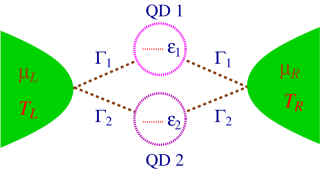
Figure 1: (color online) A quantum interferometer based on two quantum dots. Both dots are tunnel-coupled to the left and right leads. The tunneling amplitudes between the dots and the leads are denoted by $\Gamma_{1}$ and $\Gamma_{2}$. Each lead is described by an equilibrium Fermi-Dirac distribution with temperature $T_{L}$ and $T_{R}$ and electrochemical potential $\mu_{L}$ and $\mu_{R}$. The energy level position in each dot is measured as $\varepsilon_{1}$ and $\varepsilon_{2}$ relative to the Fermi energy in the leads.

Model. We start with a general model Hamiltonian

$$H=\sum_{\alpha}H_{\alpha}\{c^{\dagger}_{k\sigma};c_{k\sigma}\}+\sum_{\alpha,j}H^{T}_{\alpha,j}+\sum_{j}H^{D}_{j}\{d^{\dagger}_{j\sigma};d_{j\sigma}\},$$ (1)

where $\alpha(=L,R)$ and $j(=1,2)$ are the indices of leads and dots. The Hamiltonians $H_{\alpha}$, $H^{D}_{j}$, and

$$H^{T}_{\alpha,j}=\sum_{k\sigma\in\alpha;j}\left[V^{\alpha}_{k,j}c^{\dagger}_{k\sigma}d_{j\sigma}+{\rm h.c.}\right],$$

respectively represent the leads, the interferometer, and tunneling between the leads and the dots. $c_{k\sigma}$ and $d_{j\sigma}$ are the annihilation operators with spin $\sigma$ for electrons in the leads and the dots.

The energy (number of electrons) flowing into the interferometer is defined as the rate of change in the energy (number of electrons) in the lead $\alpha$ Mahan : $I^{E}_{\alpha}=-{d\langle H_{\alpha}\rangle/dt}=(i/\hbar)\langle[H_{\alpha},H]\rangle$ and $I_{\alpha}=-{d\langle N_{\alpha}\rangle/dt}=(i/\hbar)\langle[N_{\alpha},H]\rangle$, where $H_{\alpha}=\sum_{k\sigma\in\alpha}\varepsilon_{k}c^{\dagger}_{k\sigma}c_{k\sigma}$ and $N_{\alpha}=\sum_{k\sigma\in\alpha}c^{\dagger}_{k\sigma}c_{k\sigma}$. The heat current flowing into the interferometer from the lead $\alpha$ is defined by

$$I^{Q}_{\alpha}=I^{E}_{\alpha}-\mu_{\alpha}I_{\alpha},$$ (2)

where $\mu_{\alpha}$ is the electrochemical potential in the lead $\alpha$. Using the Keldysh Green function $G^{<}_{k\sigma,j\sigma}(t-t^{\prime})\equiv i\langle d^{\dagger}_{j\sigma}(t^{\prime})c_{k\sigma}(t)\rangle$ which involves electron operators for the leads and for each dot, one writes the heat currents as

$$I^{Q}_{\alpha}\!\! = \!\!-\!\!\sum_{k\sigma\in\alpha}\!\!\int\!\!\frac{d\varepsilon}{2\pi\hbar}(\varepsilon_{k}-\mu_{\alpha})\left[V_{k,1}G^{<}_{k\sigma,1\sigma}(\varepsilon)+{\rm h.c.}\right]$$ (3)

$$\!\!-\!\!\sum_{k\sigma\in\alpha}\!\!\int\!\!\frac{d\varepsilon}{2\pi\hbar}(\varepsilon_{k}-\mu_{\alpha})\left[V_{k,2}G^{<}_{k\sigma,2\sigma}(\varepsilon)+{\rm h.c.}\right]\,.$$

The first (second) line of Eq. (3) describes heat transfer from the left lead to QD 1 (QD 2) or vice versa. Then each heat transfer can be defined as a local heat current through each dot, $I^{Q}_{\alpha,j}$. Thus the total heat current is the sum of the local heat currents through each dot, $I^{Q}_{\alpha}=I^{Q}_{\alpha,1}+I^{Q}_{\alpha,2}$. The heat current is written in terms of the electron Green functions, $G^{<}$. The heat transfer from the lead to one of the dots is then accompanied by electron dynamics including a complex trajectory through the entire interferometer, as well as a direct tunneling to the dot.

The Green functions, $G^{<}$, can be expressed in terms of the dot Green functions defined by $G_{jj^{\prime},\sigma}^{\rm r}(t-t^{\prime})=-i\theta(t-t^{\prime})\langle\{d_{j^{\prime}\sigma}(t),d_{j\sigma}^{\dagger}(t^{\prime})\}\rangle$ and $G_{jj^{\prime},\sigma}^{<}(t-t^{\prime})=i\langle d_{j^{\prime}\sigma}(t)d_{j\sigma}^{\dagger}(t^{\prime})\rangle$ Meir92 . As a consequence, a general expression of the heat current through a nanoscale electron interferometer is given by

$$I^{Q}_{\alpha} = i\sum_{jj^{\prime}\sigma}\int\frac{d\varepsilon}{2\pi\hbar}(\varepsilon-\mu_{\alpha})\Gamma_{jj^{\prime},\alpha}(\varepsilon)\left[G^{<}_{jj^{\prime},\sigma}(\varepsilon)\right.$$ (4)

$$\hskip 39.83368pt\left.+f_{\alpha}(\varepsilon)\left(G^{r}_{jj^{\prime},\sigma}(\varepsilon)-G^{a}_{jj^{\prime},\sigma}(\varepsilon)\right)\right],$$

where the tunnel couplings between the leads and the dots are denoted by $\Gamma_{jj^{\prime},\alpha}=2\pi{\cal N}V^{\alpha}_{j}V^{\alpha*}_{j^{\prime}}$ with the density of states of the lead ${\cal N}$. The Fermi-Dirac distribution functions of the leads are $f_{\alpha}(\varepsilon)=f(\varepsilon-\mu_{\alpha})$, where the chemical potentials are $\mu_{L}=-\mu_{R}=eV/2$ with applied bias $V$ between the two leads. For $i\neq j$, the terms of the current describe the interference between the electron waves through two dots. In the absence of one dot, i.e., $V_{k,1}=0$ or $V_{k,2}=0$, only the current through the other dot exists and any interference resulting from the existence of the one dot disappears. Therefore, the expression of the heat current is reduced to the heat current formula in a single dot electronic device.

Our interferometer has the two electron pathways which are allowed for electron transport from one lead to the other via two dots not being coupled to each other directly. Electron tunneling through the dots are manipulated by varying the gate voltages. The dots makes it possible to control a coherent electron passing through the two electron pathways in the interferometer where it is required to satisfy current conservation at the leads. The current conservation gives rise to a circulating current on a closed path through the dots and the leads Cho03 . To clarify the origin of the circulating electric/heat currents in the interferometer the intradot electron-electron interaction is not taken into account in this study. Then the level spacing in each dot is larger than the applied bias and temperature because electron transport through a single level in the dots. Although intradot Coulomb interactions are considered in the Coulomb blockade regime, the resonant transport could be well explained in the Hatree-Fock mean-field level where the energy level of the dots can be described by a simple shift of the interaction parameter. In fact, we focus on studying the interference effects that are present for near resonant transport and employ the resonant level model to describe the dots; $H^{D}_{j}=\sum_{j\sigma}\varepsilon_{j}d^{\dagger}_{j\sigma}d_{j\sigma},$ where $\varepsilon_{1}$ and $\varepsilon_{2}$ are the level energy in each dot, measured, relative to the Fermi energy of the leads.

With the Keldysh technique for nonlinear current through the system, the local heat currents through each dot at the lead $\alpha$ are given by Meir92 ; Cho99 ,

$$I^{Q}_{\alpha,j}=\sum_{\sigma}\int\frac{d\varepsilon}{2\pi\hbar}\,(\varepsilon-\mu_{\alpha})(f_{\alpha}(\varepsilon)-f_{\alpha^{\prime}}(\varepsilon)){\cal T}_{j}(\varepsilon),$$ (5)

and similarly the local electric currents are obtained as

$$I_{\alpha,j}=e\sum_{\sigma}\int\frac{d\varepsilon}{2\pi\hbar}\,(f_{\alpha}(\varepsilon)-f_{\alpha^{\prime}}(\varepsilon)){\cal T}_{j}(\varepsilon),$$ (6)

where the local transmission spectral functions are defined by ${\cal T}_{j}(\varepsilon)=\left\{\mbox{\boldmath$\Gamma$}^{L}{\bf G}^{\rm r}_{\sigma}(\varepsilon)\mbox{\boldmath$\Gamma$}^{R}{\bf G}^{\rm a}_{\sigma}(\varepsilon)\right\}_{jj}$ which is the $j$-th diagonal component of the matrix transmission spectral function. ${\bf G}^{\rm r}_{\sigma}(\varepsilon)$ is the matrix dot Green function defined in time space as $G_{jj^{\prime},\sigma}^{\rm r}(t-t^{\prime})=-i\theta(t-t^{\prime})\langle\{d_{j^{\prime}\sigma}(t),d_{j\sigma}^{\dagger}(t^{\prime})\}\rangle$. The matrix coupling to the leads is described by ${\bf\Gamma}^{L}={\bf\Gamma}^{R}=\left(\begin{array}[]{cc}\Gamma_{1}&\sqrt{\Gamma_{1}\Gamma_{2}}\\ \sqrt{\Gamma_{1}\Gamma_{2}}&\Gamma_{2}\end{array}\right)$. The symmetric tunnel-coupling between the dots and the leads will be assumed to be independent of energy. The matrix Green function of the dots is

$${\bf G}_{\sigma}^{\rm r}(\varepsilon)=\left(\begin{array}[]{cc}\varepsilon-\varepsilon_{1}+i\Gamma_{1}&i\sqrt{\Gamma_{1}\Gamma_{2}}\\ i\sqrt{\Gamma_{1}\Gamma_{2}}&\varepsilon-\varepsilon_{2}+i\Gamma_{2}\end{array}\right)^{-1}.$$ (7)

From the relation, ${\bf G}_{\sigma}^{\rm a}(\varepsilon)=[{\bf G}_{\sigma}^{\rm r}(\varepsilon)]^{\dagger}$, the advanced Green function can be obtained. Accordingly, the local transmission spectral functions in terms of the total transmission function are given by

$${\cal T}_{1}(\varepsilon) = {\Gamma_{1}(\varepsilon-\varepsilon_{2})\over\Gamma_{2}(\varepsilon\!-\!\varepsilon_{1})+\Gamma_{1}(\varepsilon\!-\!\varepsilon_{2})}{\cal T}(\varepsilon),$$ (8)

$${\cal T}_{2}(\varepsilon) = {\Gamma_{2}(\varepsilon-\varepsilon_{1})\over\Gamma_{2}(\varepsilon\!-\!\varepsilon_{1})+\Gamma_{1}(\varepsilon\!-\!\varepsilon_{2})}{\cal T}(\varepsilon).$$ (9)

The total current is the sum of current through each dot, $I^{Q}=I^{Q}_{1}+I^{Q}_{2}$, which is just the current conservation. This leads to the total transmission spectral function as ${\cal T}(\varepsilon)={\cal T}_{1}(\varepsilon)+{\cal T}_{2}(\varepsilon)$,

$${\cal T}(\varepsilon)\!=\!\!{\left[\Gamma_{2}(\varepsilon\!-\!\varepsilon_{1})\!+\!\Gamma_{1}\!(\varepsilon\!-\!\varepsilon_{2})\right]^{2}\over(\varepsilon\!-\!\varepsilon_{1})^{2}(\varepsilon\!-\!\varepsilon_{2})^{2}\!+\!\left[\Gamma_{2}(\varepsilon\!-\!\varepsilon_{1})+\Gamma_{1}(\varepsilon\!-\!\varepsilon_{2})\right]^{2}}.$$ (10)

In the linear response regime, the transport electric/heat currents are expanded up to the linear terms of $\Delta T=T_{L}-T_{R}$ and $\Delta V=V_{L}-V_{R}$. The electric currents and the heat currents are related to the chemical potential difference, $\Delta V$, and the temperature difference, $\Delta T$, by the thermo-electric coefficients $L_{mm^{\prime}}$ :

$$\left(\begin{array}[]{c}I\\ I^{Q}\end{array}\right)=\left(\begin{array}[]{cc}L_{11}&L_{12}\\ L_{21}&L_{22}\end{array}\right)\left(\begin{array}[]{c}\Delta V\\ \Delta T\end{array}\right).$$ (11)

Similarly, with the local thermo-electric coefficients $L^{(j)}_{mm^{\prime}}$ the local electric/heat currents in the linear response regime can be written as

$$\left(\begin{array}[]{c}I_{j}\\ I^{Q}_{j}\end{array}\right)=\left(\begin{array}[]{cc}L^{(j)}_{11}&L^{(j)}_{12}\\ L^{(j)}_{21}&L^{(j)}_{22}\end{array}\right)\left(\begin{array}[]{c}\Delta V\\ \Delta T\end{array}\right).$$ (12)

The thermo-electric coefficients associated with the local current through each dot are expressed as $L^{(j)}_{11}=e^{2}{\cal L}^{(j)}_{0}$, $L^{(j)}_{21}=TL^{(j)}_{12}=-e{\cal L}^{(j)}_{1}$, and $L^{(j)}_{22}={\cal L}^{(j)}_{2}/T$, where the integrals are defined as ${\cal L}^{(j)}_{n}(T)=\frac{2}{h}\int d\varepsilon\left(-\frac{\partial f}{\partial\varepsilon}\right)\varepsilon^{n}{\cal T}_{j}(\varepsilon)$. According to the current conservations, the thermo-electric coefficients have the relations: $L_{mm^{\prime}}=L^{(1)}_{mm^{\prime}}+L^{(2)}_{mm^{\prime}}$.

Figure 2: Thermopower of the interferometer as a function of temperature for different level positions of the dots, $(\varepsilon_{1}/\Gamma,\varepsilon_{2}/\Gamma)$. The tunneling amplitudes are taken as $\Gamma=\Gamma_{1}=\Gamma_{2}$. For both energy levels of dots being above (below) the Fermi energy, the sign of the thermopower is negative (positive). The charge and heat are carried mainly through the electron (hole) channels. When the energy level of one dot is lying below the Fermi energy and that of the other is lying above the Fermi energy, the sign of the thermopower is changed as the temperature varies. Therefore, the main propagating channels for charge and heat determine the sign of the thermopower. The magnitude of the thermopower is of the order of $k_{B}/e=86.17\mu{\rm V}/K$.

Thermopower. The thermopower of the interferometer can be found by measuring the induced voltage drop across the interferometer when the temperature difference between two leads is applied. For zero electric transport current, $I=0$, the thermopower is defined by the relation

$$S=-\lim_{\Delta T\rightarrow 0}\frac{\Delta V}{\Delta T}\bigg{|}_{I=0}=\frac{L_{12}}{L_{11}}.$$ (13)

In terms of the defined integrals, one can rewrite the thermopower, $S=-(k_{B}/e)({\cal L}_{0}/k_{B}T{\cal L}_{1})$ with the constant $k_{B}/e\simeq 86.17\mu V/K$. In Fig. 2, the characteristics of the thermopower are shown to be dependent on the energy level positions of the dots. The sign of the thermopower can indicate the main channel in transporting charge and heat. When more transmission spectral weight lies in the electron channel then in the hole channel, the charge and heat are carried by mainly electron channels. In this case the sign of the thermopower is negative. In the opposite case, since charge and heat transport through the hole channels is predominant, the thermopower is positive. If the same amount of electron and heat are carried by each electron and hole channel, the sign of the electric/heat current is the same/opposite for electron and hole channel. This results in the thermopower being zero. As shown in Fig. 2, when the energy level of one dot is lying below the Fermi energy and that of the other dot is lying above the Fermi energy, the sign of the thermopower is changed as temperature increases.

Figure 3: (a) Local electric currents induced by a temperature gradient as a function of temperature. The dot energy levels are taken as $(\varepsilon_{1}/\Gamma,\varepsilon_{2}/\Gamma)=(-0.9,0.3)$ for the tunneling amplitudes, $\Gamma=\Gamma_{1}=\Gamma_{2}$. In contrast to the thermopower (compare Fig. 2), the level positions taken in this plot do not affect the physics of the local currents but only change its amplitude and sign. Even when the total electric transport current is zero $(I=0)$, the non-vanishing local electric currents indicates the existence of the circulating electric current which makes the interferometer magnetically polarized. The magnetic polarization current is then defined as the local current: $I_{M}\equiv I_{1}=-I_{2}$ for $I=0$. (b) The ratio of the magnetic polarization currents to the temperature gradient, $\Delta T$, as a function of temperature. The magnitude of the magnetic polarization currents is of the order of ${\rm nA}$ for a temperature gradient of order $1{\rm K}$.

Local electric currents and magnetic polarization currents. The requirement, that the electric transport current is zero, for the thermopower implies that the local electric currents are required to ensure $I_{1}=-I_{2}$. If these local currents exist for $I=0$, the local electric currents should circulate on the closed path through the leads and the dots. Then the interferometer can be magnetized by the circulating electric currents. One can define the circulating current as a magnetic polarization current Cho03 , $I_{M}\equiv I_{1}=-I_{2}$ for $I=0$. From Eq. (11), the magnetic polarization current is then expressed as

$$I_{M}={\cal K}\,\Delta T,$$ (14)

where ${\cal K}=-SL^{(1)}_{11}+L^{(1)}_{12}=SL^{(2)}_{11}-L^{(2)}_{12}$. This shows that the magnetic polarization current exists even when the electric transport current is zero because this magnetic polarization current is induced by the temperature gradient between the leads due to the quantum interference. Figure 3(a) shows that the total sum of the local currents is always zero because the local electric currents are flowing along the opposite direction to each other, which implies the existence of the magnetic polarization current. It should be noted that the direction of the magnetic polarization current is reversed as the temperature increases. If one can define the local thermopower as $S_{j}=L^{(j)}_{12}/L^{(j)}_{11}$, the magnetic polarization current vanishes at a specific temperature, $T_{0}$, satisfying $S(T_{0})=-S_{j}(T_{0})$. It is also shown in Fig. 4 (b) that, by manipulating the gate voltages of each dot, the magnetic polarization current can be controlled. This implies that changing the energy level positions of each dot, one can magnetize the interferometer by the magnetic polarization current induced by the temperature gradient as up-, non-, and down-polarized. In contrast to the measurement of the thermopower by means of electron transport, to observe the magnetic polarization current, one can measure a magnetic field produced by the magnetic polarization current by using a superconducting quantum interference device (SQUID). Recent measurements of a persistent current by using a SQUID Rabaud01 show that magnitudes of the magnetic polarization current of the order of ${\rm nA}$ should be experimentally observable for a temperature gradient of order $0.1\sim 1{\rm K}$.

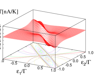
Figure 4: (color online) The ratio of the magnetic polarization current $I_{M}\equiv I_{1}=-I_{2}$ to the temperature gradient $\Delta T$ for $I=0$ as a function of the energy level positions of each dot $(\varepsilon_{1}/\Gamma,\varepsilon_{2}/\Gamma)$ for $k_{B}T=5.0\times 10^{-2}\Gamma$. The tunneling amplitudes are taken as $\Gamma=\Gamma_{1}=\Gamma_{2}$. Note that by varying the energy level of each dot the interferometer has a different magnetic state according to the direction of the magnetic polarization current.

Heat currents. The condition of an open circuit ($I=0$) to find the thermopower can apply for a circulating heat current in the interferometer. Under the condition, $I=0$, the local heat currents are rewritten as

$$I^{Q}_{j}=\kappa_{j}\Delta T,$$ (15)

where $\kappa_{j}=-SL^{(j)}_{21}+L^{(j)}_{22}$. Due to the quantum interference, the local heat currents can be greater than the total heat current through the interferometer at a given energy level positions of the dots. If $I^{Q}_{1}>I^{Q}$, there exists an excess heat current through QD 1. One can define the excess current as $I^{Q}_{exe}=I^{Q}_{1}-I^{Q}$. From the relation $I^{Q}=I^{Q}_{1}+I^{Q}_{2}$, the local heat current through the QD 2 should be $I^{Q}_{2}=-I^{Q}_{exe}$. The negative sign of the local heat current through the QD 2 implies that the heat current conservation requires a heat current flowing through the QD 2 against the temperature gradient. According to the second law of the thermodynamics, the entropy production defined by $I^{S}\equiv I^{Q}/T>0$ should be greater than zero during thermoelectric process Guttman . If one can define a local entropy production as $I^{S}_{j}\equiv I^{Q}_{j}/T$, the local heat current flowing against the temperature gradient means that $I^{S}_{2}<0$. However, for heat transfer through the entire interferometer, the heat current conservation should make the second law of the thermodynamics preserved in heat transport through the entire interferometer. As a result, the excess heat transport through the QD 1 is compensated with the local heat current flowing against the temperature gradient through the QD 2. Like the magnetic polarization current, those thermoelectric processes imply that there appears a circulating heat current on the closed path between the dots and the leads in order to satisfy the second law of the thermodynamics. Therefore, for $I^{Q}_{1}>I^{Q}$, the excess current can be defined as a circulating heat current, $I^{Q}_{M}\equiv I^{Q}_{exe}=-I^{Q}_{2}$. Similarly, for $I^{Q}<I^{Q}_{2}$, the circulating heat current is determined. In Fig. 5, we display the circulating heat current as a function of the energy level positions of each dot from the numerical calculation. It is shown that the interference between the electron and hole channels produces the circulating heat current.

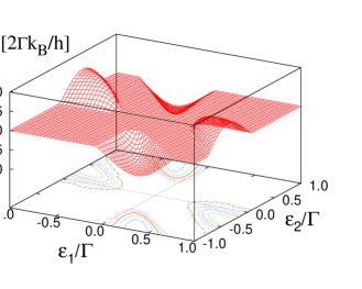
Figure 5: (color online) The ratio of the circulating heat current to the temperature gradient $\Delta T$ as a function of the energy level positions of each dot $(\varepsilon_{1}/\Gamma,\varepsilon_{2}/\Gamma)$ for $I=0$. The parameters are taken as $k_{B}T=5.0\times 10^{-2}\Gamma$ and $\Gamma=\Gamma_{1}=\Gamma_{2}$. The existence of the circulating heat current indicates that while the local heat current through one dot can be greater than the total transport heat current through the interferometer due to the quantum interference, the local heat current through the other dot flows against the temperature gradient. The current conservation requires that the local excess heat current circulate on the closed path in the interferometer.

Summary. We have investigated thermal transport in nanoscale interferometers. The expression of the heat current for the interferometer has been derived based on the nonequilibrium Green’s function technique. Controllable electronic states in two dots make it possible to manipulate the quantum interference which causes a heat current in the opposite direction to the temperature drop through one dot and an excess heat current through the other dot. The circulating electric current induced by a temperature gradient across the entire interferometer is sufficiently large that it should be experimentally observable.

Note added. After completion of this work, we become aware of some related work by Moskalets concerning a temperature-induced circulating electric current in a one-dimensional ballistic ring Moskalets1 .

Acknowledgments. This work was supported by the University of Queensland and the Australian Research Council.

References

- (1) See, for a review, Y. Imry, Introduction to Mesoscopic Physics, 2nd ed. (Oxford University Press, Oxford, New York 2002); S. Datta, Electronic Transport in Mesoscopic Systems (Cambridge University Press, New York 1995).
- (2) A. Yacoby, M. Heiblum, D. Mahalu, and H. Shtrikman, Phys. Rev. Lett. 74, 4047 (1995).
- (3) R. Schuster, E. Buks, M. Heiblum, D. Mahalu, V. Umansky, H. Shtrikman, Nature 385, 417 (1997).
- (4) E. Buks, R. Schuster, M. Heiblum, D. Mahalu, and V. Umansky, Nature 391, 871 (1998).
- (5) W.G. van der Wiel, S. De Franceschi, T. Fujisawa, J.M. Elzerman, S. Tarucha, and L.P. Kouwenhoven, Science 289, 2105 (2000); Y. Ji, M. Heiblum, D. Sprinzak, D. Mahalu, and H. Shtrikman, Science 290, 779 (2000).
- (6) A.W.Holleitner, C. R. Decker, H. Qin, K. Eberl, and R.H. Blick, Phys. Rev. Lett. 87, 256802 (2001).
- (7) B. Kubala and J. König, Phys. Rev. B 65, 245301 (2002).
- (8) H. Akera, Phys. Rev. B 47, 6835 (1993).
- (9) W. Izumida, O. Sakai, and Y. Shimizu, J. Phys. Soc. Japan 66, 717 (1997).
- (10) S. Y. Cho, R. H. McKenzie, K. Kang, and C. K. Kim, J. Phys.: Condensd Matter 15, 1147 (2003).
- (11) D. Loss and E.V. Sukhorukov, Phys. Rev. Lett. 84, 1035 (2000).
- (12) U. Sivan and Y. Imry, Phys. Rev. B 33, 551 (1986).
- (13) C. W. J. Beenakker and A. A. M. Staring, Phys. Rev. B 46, 9667 (1992).
- (14) G.D. Guttman, E. Ben-Jacob, and D.J. Bergman, Phys. Rev. B 51, 17758 (1995).
- (15) M. V. Moskalets, JETP 87, 991 (1998) [Soviet Zh. Eksp. Teor. Fiz. 114, 1827 (1998)].
- (16) N. J. Appleyard, J. T. Nicholls, M. Y. Simmons, W. R. Tribe, and M. Pepper, Phys. Rev. Lett. 81, 3491 (1998).
- (17) K. Schwab, E. A. Henriken, J. M. Worlock, and M. L. Roukes, Nature 404, 974 (2000).
- (18) A. V. Andreev and K. A. Matveev, Phys. Rev. Lett. 86, 280 (2001).
- (19) T.-S. Kim and S. Hershfield, Phys. Rev. Lett. 88, 136601 (2002).
- (20) K. A. Matveev and A. V. Andreev, Phys. Rev. B 66, 045301 (2002).
- (21) T. E. Humphrey, R. Newbury, R. P. Taylor, and H. Linke, Phys. Rev. Lett. 89, 116801 (2002).
- (22) G. M. Wang, E. M. Sevick, Emil Mittag, Debra J. Searles, and Denis J. Evans, Phys. Rev. Lett. 89, 050601 (2002); S. Tasaki, I. Terasaki, and T. Monnai, cond-mat/0208154 (unpublished); Th. M. Nieuwenhuizen and A. E. Allahverdyan, cond-mat/0207587 (unpublished).
- (23) Th. M. Nieuwenhuizen and A. E. Allahverdyan, Phys. Rev. E 66, 036102 (2002).
- (24) A. E. Allahverdyan and Th. M. Nieuwenhuizen, Phys. Rev. B 66, 115309 (2002).
- (25) G. D. Mahan, Many-Particle Physics, 2nd ed. (Plenum, New York 1990), p. 227.
- (26) Y. Meir, and N. S. Wingreen, Phys. Rev. Lett. 68, 2512 (1992).
- (27) S. Y. Cho, K. Kang, and C.-M. Ryu, Phys. Rev. B 60, 16874 (1999).
- (28) W. Rabaud, L. Saminadayar, D. Mailly, K. Hasselbach, A. Benoit, and B. Etienne, Phys. Rev. Lett. 86, 3124 (2001).
- (29) M. V. Moskalets, Europhys. Lett. 41, 189 (1998).