Interacting damage models mapped onto Ising and percolation models

Abstract

We introduce a class of damage models on regular lattices with isotropic interactions between the broken cells of the lattice. Quasistatic fiber bundles are an example. The interactions are assumed to be weak, in the sense that the stress perturbation from a broken cell is much smaller than the mean stress in the system. The system starts intact with a surface-energy threshold required to break any cell sampled from an uncorrelated quenched-disorder distribution. The evolution of this heterogeneous system is ruled by Griffith’s principle which states that a cell breaks when the release in potential (elastic) energy in the system exceeds the surface-energy barrier necessary to break the cell. By direct integration over all possible realizations of the quenched disorder, we obtain the probability distribution of each damage configuration at any level of the imposed external deformation. We demonstrate an isomorphism between the distributions so obtained and standard generalized Ising models, in which the coupling constants and effective temperature in the Ising model are functions of the nature of the quenched-disorder distribution and the extent of accumulated damage. In particular, we show that damage models with global load sharing are isomorphic to standard percolation theory, that damage models with local load sharing rule are isomorphic to the standard Ising model, and draw consequences thereof for the universality class and behavior of the autocorrelation length of the breakdown transitions corresponding to these models. We also treat damage models having more general power-law interactions, and classify the breakdown process as a function of the power-law interaction exponent. Last, we also show that the probability distribution over configurations is a maximum of Shannon’s entropy under some specific constraints related to the energetic balance of the fracture process, which firmly relates this type of quenched-disorder based damage model to standard statistical mechanics.

I Introduction

The physics of breakdown processes that lead, for example, to stress-induced catastrophic failure of man-made and geological structures, remains an ongoing subject of research. Stress-induced fracture of a homogeneous material containing a geometrically simple single flaw has been studied since the work of Griffith Griffith (1920) and is now well understood. However, the breakdown of heterogeneous structures, in which the local mechanical properties are randomly distributed in space and/or time, continues to present challenges despite the many advances over the last fifteen years Herrmann and Roux (1990). The difficulty is in characterizing and quantifying the effects of interaction between the multitude of constituents.

Most of the knowledge about these types of systems has been obtained from lattice network simulations. One of the most well-studied lattice network models is the 80 year old Fiber Bundle Model (FBM) Daniels (1945, 1989); Coleman (1958); Peirce (1926) that describes the rupture of bundles of parallel fibers. This model originally considered elastic fibers of identical elastic constant, breaking when their elongation exceeds individual thresholds distributed according to a given uncorrelated random distribution. A global load sharing rule (GLS) is assumed by which the load carried by a fiber is uniformly distributed to the surviving fibers when it breaks. Analytical results for this model have been obtained Sornette (1989, 1992); Andersen et al. (1997); Hemmer and Hansen (1992); Pride and Toussaint (2002) that concern the average load/deformation properties Sornette (1989, 1992); Andersen et al. (1997), the distribution of avalanches Hemmer and Hansen (1992), or the relationship between such quenched-disorder based models and standard statistical mechanics Pride and Toussaint (2002).

The original FBM model with global-load sharing has been generalized to allow for non-uniform load sharing rules, considered either as purely local load sharing (LLS), in which case distribution of avalanches and mechanical properties have been analytically studied Hansen and Hemmer (1994); Kloster et al. (1997); Zhang and Ding (1996), or as power laws of distance from the failed fiber, which have been studied numerically Hidalgo et al. (2002); Yewande et al. (2003). The distribution of avalanche size $s$ has been shown to be a power law $s^{-5/2}$ close to macroscopic breakdown in GLS, and not to follow any power-law in LLS Kloster et al. (1997); Hansen and Hemmer (1994).

Closely related to these models of fiber bundles in elastic interaction, many studies have addressed fuse networks Bakke et al. (2003); Batrouni and Hansen (1998); De Arcangelis and Herrmann (1989); De Arcangelis et al. (1989); Duxbury et al. (1987); Hansen and Schmittbuhl (2003); Hansen et al. (1991); Zapperi et al. (2000, 2003), or networks of isotropic damage with interactions having the range of the elastostatic Green function Batrouni et al. (2002); Herrmann et al. (1989); Schmittbuhl et al. (2003). Such work has recently helped to understand the origin of a universal geometric feature of crack surfaces; namely, their large-scale self-affinity. It is now established that three-dimensional fracture surfaces in disordered brittle solids are self-affine, with a material-independent roughness exponent $\zeta\sim 0.8$ at large scales Bouchaud (1997); Schmittbuhl et al. (1995, 1993); Lea Cox and Wang (1993); Måløy et al. (1992); Bouchaud et al. (1990), and a cross-over to $\zeta\sim 0.5$ at smaller scales. Daguier et al. (1996, 1997) In another load geometry, interfacial crack pinning between two sintered PMMA plates have been reported to give rise to crack fronts with $\zeta\sim 0.6$ Schmittbuhl and Måløy (1997); Delaplace et al. (1999). Recent work Hansen and Schmittbuhl (2003); Schmittbuhl et al. (2003) has explained these large-scale roughness exponents using gradient-percolation theory (Sapoval et al. (1985), relationship to fracture problems first introduced in Refs. Zapperi et al. (2000, 2003)), together with estimates of the correlation-length divergence exponent obtained using finite-size scaling of lattice models in the approach to failure. Scaling laws were produced relating the roughness exponents of fracture or damage fronts, to the critical exponent describing the divergence of an autocorrelation length in an appropriate damage model. Thus, one important objective of the present work is to analytically extract such divergence exponents for a broad class of damage models and to show how such exponents depend on the model characteristics.

The classification of lattice breakdown processes as critical-point phenomena is still subject to debate Moreno et al. (2001, 2000); Zapperi et al. (1997a); Zapperi et al. (1999); Zapperi et al. (1997b); Kun et al. (2000); Andersen et al. (1997); Sornette and Andersen (1998); Caldarelli et al. (1996); Räisänen et al. (1998). Local load sharing models are usually understood as breaking through a process similar to a first-order transition Moreno et al. (2001), while models with long-range elastic interactions or GLS are analyzed either as a critical-point transition Moreno et al. (2001, 2000); Sornette and Andersen (1998); Andersen et al. (1997), or as a spinodal nucleation process Zapperi et al. (1997a); Rundle and Klein (1989). The issue depends on whether the accumulated damage has a correlation length that diverges as a power law of the average deformation in the approach to macroscopic failure. Numerical evidence in the literature suggests that the nature of the correlation length in the approach to failure depends on the specific model being analyzed, the damage interaction range, and the type of quenched-disorder distribution considered. A major difficulty of such attempts to classify the breakdown process is that no analytic form for the distribution of the damage configurations at a given external load is available (at least that has a firm basis). Numerical simulations of the scaling behavior of avalanches are limited in size due to computational restrictions which makes critical-point analysis difficult.

It is proven here that quasi-static interacting damage models, that possess local breaking thresholds randomly quenched ab initio, can be mapped onto percolation, Ising or generalized Ising models with non-zero coupling constants for distant cells, depending on the range of the assumed load sharing rule and on the specific probability distribution of the breaking thresholds. The stress-induced emergent-damage distribution is proven here to be a Boltzmannian with a temperature (probabilistic energy scale) that is an explicit analytical function of the applied external load. Having an analytical form for the damage-state distribution function allows a rigorous classification of the breakdown process into first-order or critical-point phase transitions belonging to various universality classes.

We have recently proposed a statistical theory for the localization of oriented fractures that emerge and elastically interact when the system has a shear stress applied to it Toussaint and Pride (2002a, b, c). The distribution of the emergent crack states was obtained using the postulate that the fracture arrival would maximize Shannon’s entropy under constraints representing the energetic balance of the process. In the present work, we will not make this postulate but will instead prove its validity by direct integration over the damage evolution. The present work also presents more general ranges of interaction. However, unlike our previous work, the present analysis is for a purely scalar description of damage interaction. The interaction of real fractures in an anisotropic load, where microfractures present high aspect ratios, necessarily requires a tensorial elastic description as our earlier work Toussaint and Pride (2002a, b, c) provided.

Other analytical treatments of fracture processes in disordered brittle materials can be found in the literature Rundle and Klein (1989); Blumberg Selinger et al. (1991). These approaches directly postulate both the appropriateness of classical Boltzmann distributions and the form of a free energy containing non-local long-range interactions. Such approaches have led to the analysis of fracture processes as a spinodal nucleation. However, the mechanical origin of such a free energy and its relation to the underlying presence of fractures and heterogeneity in the system, as well as the physical meaning of the temperature parameter, remain unclear in these models. Fractures usually form irreversibly, which makes such direct applications of standard equilibrium statistical mechanics questionable. Fracture theories as a thermally activated process Griffith (1920); Pomeau (1992) have long been proposed. However, the pertinence of thermal activation in highly heterogeneous and stiff systems is doubtful, because the thermal energy is negligeable compared to the gaps between the strain energies of the possible states of the system.

Thermally induced fracture models Pomeau (1992), generalized with quenched disorder in the rupture thresholds Roux (2000); Politi et al. (2002); Santucci et al. (2003); Ciliberto et al. (2001), have recently been confronted with experiments. Microacoustic emissions in heterogeneous materials prior to failure were experimentally observed to have a cumulative energy that follows a power law in time to failure, while the individual microacoustics events have energies distributed as a power law Guarino et al. (2002, 1998); Garcimartin et al. (1997). In models reproducing these experimental results through time-delayed fiber bundles with GLS, it has been pointed out that the type of quenched-disorder distribution assumed for the individual failure thresholds directly influences the equivalent temperature in thermally activated rupture models Roux (2000); Politi et al. (2002); Santucci et al. (2003); Ciliberto et al. (2001), which makes this temperature significantly different from the usual temperature associated with molecular motion.

In comparison with these latter works, the models developed here are quasistatic and do not include any time-delayed fracture processes, but their advantage is the consideration of an arbitrary range of interactions and of arbitrary distribution functions for the fracture thresholds (similar to Refs. Hidalgo et al. (2002); Yewande et al. (2003), except that the present work is analytical rather than numerical). The nature of the energy scale (called temperature) that enters the probability distribution will also be clarified.

The organization of the paper is as follows: in section II, we introduce (and justify in the appendix) the general type of scalar damage models that are considered. In section III, the probability of each damage configuration is obtained by integrating over all paths that lead to it. In section IV, we establish the relationship between these configurational distributions and standard statistical mechanics, which allows the standard toolbox of statistical mechanics to be applied to damage models entirely based on quenched disorder. These analytical developments will then be utilized in section V to establish that fracture processes in such damage models are isomorphic to percolation for GLS (V.1), or to the Ising model for LLS (V.2). This allows us to isolate some transition points in these models, and to predict the nature of the correlation length in the approach to the transition. We will also discuss in Section V.3 the case of damage models with arbitrary power-law decay of the interactions, and show how they are related to generalized Ising models, which can themself be mapped onto standard ones via renormalization of the coupling constants. The results are summarized and discussed in a concluding section.

II Definition of the damage models considered

Our models reside on a regular lattice of dimension $D$ (e.g., a square lattice in $D=2$). Each cell of the lattice has a location $x$ within the ensemble $\Omega$ of cells making up the lattice, and has a state described by a local order parameter $\varphi_{x}$, where $\varphi_{x}=0$ if the cell is intact and $\varphi_{x}=1$ if it is broken. There is a local stress and strain associated with each cell. The cells elastically interact with each other; however, such interaction must be isotropic for the present analysis to apply. A configuration of damage is described as a damage field $\varphi$ corresponding to the set of $N$ local variables $\varphi\equiv\left\{\varphi_{x}\right\}_{x\in\Omega}$ where $N=\text{Card}(\Omega)$ is the total number of cells in the system.

Our systems are initially uniform by hypothesis; i.e., they have a homogeneous damage field $\varphi=0$ at zero strain and stress and each cell starts with the same elastic moduli. Strain is progressively applied through the application of a uniform normal displacement $l$ at the edges of the system. A cell breaks at constant applied $l$ when the energy required to break it (which is a random quenched threshold sampled from a probability distribution function) just equals the reduction in stored elastic energy in the lattice due to the break.

A key requirement of the class of models treated here is that the stress perturbation emanating from a broken cell must be weak enough that a first Born approximation holds. This means that the stress interaction between any two broken cells is allowed for while simultaneous interaction between three or more broken cells is not. This approximation is valid whenever the stress perturbation due to a broken site is much smaller than the mean stress in the system.

One specific realization of such a “weak damage” model is an appropriately defined fiber bundle model. In the model, a set of $N$ elastic fibers are stretched between a free rigid plate and an elastic halfspace. The rigid plate is displaced by a controlled amount $l$ that puts the fibers in tension. Once fibers begin to break, elastic interactions occur through the elastic solid. As demonstrated in the appendix, such interactions will be weak if either: (1) the elastic solid is much stiffer than the fiber material; or, (2) the fibers are much longer than wide and are sufficiently widely placed. In the limit that the elastic halfspace becomes rigid, this model reduces to the classic global-load sharing fiber bundle.

Another realization is a uniform elastic isotropic solid divided into $N$ cells. Uniform displacements $l$ are applied normally to the limiting faces of the lattice in such a way that the material is in a state of uniform dilation. The damage that arrives is assumed to change the isotropic moduli without creating anisotropy in the process. For example, the damage might be modeled as a spherical cavity that opens at the center of the cell thus reducing the elastic moduli of that cell. The weak interaction is guaranteed if the change in the cell modulus is small. This can be considered a special case of the oriented damage models we have considered in earlier work Toussaint and Pride (2002a, b, c).

As demonstrated in the appendix, the energy $E_{p}$ reversibly stored in such systems when the system is in a damage state $\varphi$ at the applied loading level $l$ is

$$E_{p}[\varphi,l] = (C_{0}+C_{1}+C_{2})l^{2}$$ (1)

$$C_{0} = N$$ (2)

$$C_{1} = -c\sum_{x\in\Omega}\varphi_{x}$$ (3)

$$C_{2} = -\varepsilon\sum_{x,y}J_{xy}\varphi_{x}\varphi_{y}$$ (4)

where $c$ is a positive constant in the range $0<c\leq 1$ that is independent of the damage/deformation state, $\varepsilon$ is a small positive parameter in the range $0<\varepsilon/c\ll 1$ that controls the strength of the stress perturbations, and $J_{xy}$ are $O(1)$ coupling constants that allow for the load redistribution between cells at positions $x$ and $y$ when a cell is broken. Various spatial ranges for $J_{xy}$ are considered including: (1) global load sharing in which case $J_{xy}=0$; (2) local load sharing in which case $J_{xy}=\alpha>0$ is a constant of order unity for pairs $xy$ of nearest neighbors, $0$ otherwise; (3) elastic load sharing in which case $J_{xy}\sim(\ell/|x-y|)^{D}$ where $\ell$ is the lattice step size; and (4) fiber-bundle elastic sharing with fibers interacting through an elastic plate in which case $D=2$ and $J_{xy}\sim\ell/|x-y|$ [see the appendix].

The local load sharing case (2) can in principle happen in a fiber bundle stretched between plates enduring both elastic and plastic deformations capable of screening the stress perturbations caused by broken fibers to only nearest neighbors, which always can carry some load if damaging them only decreases their elastic constant (i.e. $c<1$). We treat case (2) for the sake of generality and do not specify the detailed constitutive relations required for it to be realized in practice.

The cost in surface energy to break any of the cells (which represents either the energy required to create new surface area within a cell or to break a fiber) is a random variable fixed ab initio, with no spatial correlations between the different cells. The breaking energy is thus a quenched uncorrelated disorder, described by a probability distribution function $p(e)$ for which $p(e)de$ is the probability that a cell’s surface energy is in $[e,e+de]$, and having a cumulative distribution $P(e)=\int_{0}^{e}p(z)dz$. For a given realization of each cell’s surface energy $e_{x}$, there is thus a certain total surface energy

$$E_{s}[\varphi]=\sum_{x\in\Omega}e_{x}(1-\varphi_{x})$$ (5)

associated with each damage field $\varphi=\left\{\varphi_{x}\right\}_{x\in\Omega}$.

Given that $B\subset\Omega$ is a certain subset of locations, the notation $\varphi^{B}$ refers to the state where this subset is broken and its complementary intact; i.e., $\varphi_{x}^{B}=1$ for every $x\in B$, and $\varphi_{x}^{I}=0$ for every $x\in I=B^{C}$.

As the external deformation $l$ is increased, damage evolution is ruled by Griffith’s principle: Given that the system is in a certain configuration $\varphi^{B}$, at a given deformation $l$, it can undergo a transition towards a more broken state $\varphi^{B\cup\left\{x\right\}}$ differing from the previous one by one additional broken cell at $x$, if the release in potential energy is equal to the surface energy cost of the new break; i.e., if

$$\Delta E_{p}[\varphi^{B},x,l]=e_{x}$$ (6)

where

$$\Delta E_{p}[\varphi^{B},x,l] = E_{p}[\varphi^{B},l]-E_{p}[\varphi^{B\cup\left\{x\right\}},l]$$ (7)

$$= (c+\varepsilon\sum_{y}J_{xy}\varphi_{y})l^{2}.$$

If $e_{x}>\Delta E_{p}[\varphi^{B},x,l]$ for any surviving cell $x\in I$, there is no break and the deformation can be further increased while the system remains in the same state $\varphi^{B}$. If a break happens in cell $x$, which leads to the new state $\varphi^{E}$ where $E=B\cup\left\{x\right\}$ while the external deformation $l$ is kept constant, there is a possibility of avalanche at fixed $l$ if there is some $y\in E^{C}$ such that

$$\Delta E_{p}[\varphi^{E},y,l]\geq e_{y}.$$ (8)

If there is more than one possible location satisfying Eq. (8), the one which breaks is determined by maximizing the energy release; i.e., its location corresponds to

$$\Delta E_{p}[\varphi^{E},y,l]-e_{y}=\text{Max}_{z\in E^{C}}\left(\Delta E_{p}[\varphi^{E},z,l]-e_{z}\right).$$ (9)

The avalanche test [Eq. (8)] is then computed again until the system stabilizes in a given configuration.

Eventually, although we have chosen to base the evolution of our damage model on minimization of energy, we note that the formal integration of path probabilities presented in the following sections could similarly be obtained as well for the case of a rule based on force thresholds, with at any given external deformation, a force carried per intact fiber equal to an average one, plus perturbations due to the already broken fibers. However, this approach will not be pursued here.

III Probability distribution of damage states

The probability of occurence of any damage configuration $\varphi$ is now determined when the system is at a given external deformation $l$ that was reached monotonically ($l$ as defined here does not include any elastic unloading). We will first summarize the results for the simplest case, global load sharing, which was performed in Pride and Toussaint (2002), and which will serve as a basis for a perturbative treatment to include the effect of interactions.

III.1 Global load sharing

In this case, the interaction term of Eq. (4) is $C_{2}=0$ for any configuration, and from Eq. (7), $\Delta E_{p}[\varphi,x,l]=cl^{2}$ regardless of the state $\varphi$ and new break location $x$ considered.

Each of the cells then share the same level of deformation $l$, and the probability for any one of them to be broken is simply (from the cumulative surface energy distribution)

$$P_{0}=P(e<cl^{2})=\int_{0}^{cl^{2}}p(z)\,dz.$$ (10)

The probability of being in a configuration $\varphi$ with $n$ cells broken out of $N$ is then

$$P[\varphi,l]=P_{0}(l)^{n}(1-P_{0}(l))^{N-n}.$$ (11)

This corresponds to the behavior of a so-called “two-state system” in which each of the $N$ independent sites has a probability $P_{0}(l)$ of being broken and $1-P_{0}(l)$ of being intact. The consequences of this distribution function for the mechanical behavior and correlation length at the transition point of macroscopic rupture will be developed in section V.1.

III.2 Local load sharing

III.2.1 Damage-state probability distribution

We now consider the case where each broken cell increases the local deformation by an amount $\alpha\varepsilon l$ on each of its nearest neighbors; i.e., $J_{xy}=\alpha$ for each nearest neighbor pair, or $J_{xy}=0$ for more distant cells.

Note that for a given cell $x$, the potential energy release defined in Eq. (7), $\Delta E_{p}[\varphi,x,l]$, is a growing function of both the deformation $l$ and the subset of cracked cells $\varphi$ considered – in the sense that if we consider two subsets $B\subset D$ and $x\in D^{C}$, then $\Delta E_{p}[\varphi^{D},x,l]\geq\Delta E_{p}[\varphi^{B},x,l]$. Physically, this inequality means that the local load over each cell increases with the external load imposed, and that any cell breaking anywhere else induces an additional increase in local load. This inequality will play a key role in obtaining the damage-state probability distribution.

To aid the pedagogic development, we first derive the probability of occurence of a configuration $\varphi^{B}$ with $n$ isolated broken cells forming a subset $B$, which do not share any common nearest neighbors. There are $zn$ nearest neighbors to these $n$ cells (in a subset $F$ corresponding to the boundary of broken cells) where $z$ is the coordination number of the lattice considered. There are then $N-(z+1)n$ cells completely isolated from the broken ones in the subset $(B\cup F)^{C}$. For a cell $x$ having broken from an intermediate stage $\varphi^{A}$ with $A\subset B$, at an intermediate external load $h\in[0,l]$, the change in the stored energy satisfies $\Delta E_{p}[\varphi^{A},x,h]=ch^{2}\leq cl^{2}$. For every cell having survived, we have either $\Delta E_{p}[\varphi^{B},x,l]=(c+\alpha\varepsilon)l^{2}$ if $x\in F$ ($x$ is on the boundary of the broken cells set), or $\Delta E_{p}[\varphi^{B},x,l]=cl^{2}$ if $x\in(B\cup F)^{C}$ ($x$ is completely disconnected from the broken cells set). Applying Griffith’s principle [Eq. (6)] to every cell and intermediate deformations $h\in[0,l]$, and using the monotony of $\Delta E_{p}[\varphi,x,l]$ in both $l$ and $\varphi$, we obtain that a necessary and sufficient condition for all cells in $B$ to be broken is that their surface energy thresholds were below $cl^{2}$, while those of their neighbors in $F$ were above $(c+\alpha\varepsilon)l^{2}$, and the remaining ones in $(B\cup F)^{C}$ above $cl^{2}$. Defining

$$P_{1}(l)=P(e<(c+\alpha\varepsilon)l^{2})=\int_{0}^{(c+\alpha\varepsilon)l^{2}}p(z)\,dz,$$ (12)

this then implies that

$$P[\varphi,x]=P_{0}^{n}(1-P_{1})^{zn}(1-P_{0})^{N-(z+1)n}.$$ (13)

is the probability of occurence of such a configuration.

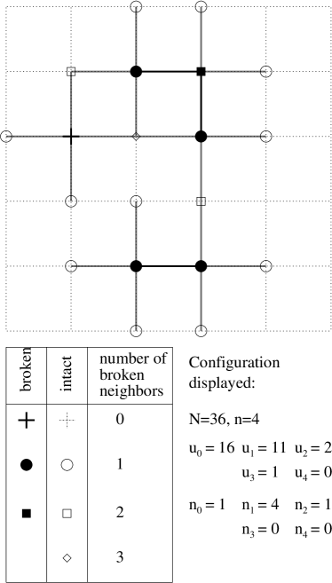
Figure 1: Typical configuration and associated connectivity measures.

We now pass to the more general case. In the argument, we obtain upper and lower bounds for the probability of some arbitrary damage state, and then demonstrate that in the limit $\varepsilon/c\ll 1$, the two bounds converge to the unique probability distribution of interest.

For any configuration $\varphi$, $u_{k}$ is defined as the number of intact cells with $k$ broken nearest neighbors and $n_{k}$ as the number of broken cells with $k$ broken neighbors. If $n$ out of the $N$ cells are broken, we have $\sum_{k}n_{k}=n$ and $\sum_{k}u_{k}=N-n$. The way the above quantities are associated to any particular configuration is illustrated in Fig. 1.

For a cell $x$ which broke from an intermediate state $\psi\subset\varphi$ with $k$ already broken neighbors in $\psi$, at an external load $h$, we have

$$\Delta E_{p}[\psi,x,h]=(c+k\alpha\varepsilon)h^{2}.$$ (14)

Using again the monotony of $\Delta E_{p}$, a necessary and sufficient condition for any intact cell $y\in B^{C}$ to have survived is that its threshold exceeded $\Delta E_{p}[\varphi,y,l]$. The probability for each of these independent statistical events to occur is expressed as $1-P_{k}(l)$, where

$$P_{k}(l)=P(e<(c+k\alpha\varepsilon)l^{2}).$$ (15)

For any cell which broke $x\in B$, we note that they have broken with certainty at the ultimate deformation $l$ if the external load was sufficient to trigger their break without the help of overload due to breaks of the other ones; i.e., they have broken with certainty if their energy threshold was below $\Delta E_{p}(\varphi^{\emptyset},x,l)=cl^{2}$ where $\emptyset$ denotes the empty set (no broken cells). Furthermore, if every threshold in $B$ was below $cl^{2}$, except a particular one $x\in B$ which has $k_{x}$ broken neighbors in the considered configuration $\varphi^{B}$ and has a breaking energy between $cl^{2}$ and $(c+k_{x}\alpha\varepsilon)l^{2}$, the $k_{x}$ neighbors of this considered cell $x$ will have broken with certainty at the ultimate load $l$, so that $x$ will also break with certainty under the effect of the overload due to its broken neighbors. The probability that this individual threshold broke under the sole effect of the overload due to its neighbors can be expressed

$$\Delta P_{k_{x}}=P_{k_{x}}(l)-P_{0}(l)$$ (16)

Thus, a lower bound for the probability of occurence of the configuration $\varphi^{B}$ can be expressed as

$$P[\varphi^{B},l]>$$ (17)

$$\left[P_{0}^{n}+\left(\sum_{x\in B}P_{0}^{n-1}\Delta P_{k_{x}}\right)\right]\prod_{k\in{N}}(1-P_{k})^{u_{k}}$$

where the index $k$ runs formally to ${N}$; however, $u_{k}=0$ when $k>z$ (the coordination number of the lattice).

For any cell $x\in B$ which broke, its associated energy threshold was necessarily lower than $\Delta E_{p}[\varphi^{B\smallsetminus\left\{x\right\}},x,l]$ where $B\smallsetminus\left\{x\right\}$ denotes the set $B$ with cell $\{x\}$ excluded from it. Thus, an upper bound for the probability of occurence of the configuration under study, is

$$P[\varphi^{B},l]<$$ (18)

$$\left[\prod_{x\in B}P_{k_{x}}\right]\prod_{k}(1-P_{k})^{u_{k}}=$$

$$\left[\prod_{x\in B}(P_{0}+\Delta P_{k_{x}})\right]\prod_{k}(1-P_{k})^{u_{k}}.$$

For a continuous p.d.f. over thresholds (that guarantees no jumps in the cumulative distribution $P$ and is the only restriction placed on the p.d.f.), $\Delta P_{k}$ is a quantity of order $\varepsilon$, and $P_{0}$ is of order $1$. In the limit of a Born model (weak stress perturbations for which $\varepsilon/c\ll 1$), the upper and lower bounds for the probability of occurence are identical to order $\varepsilon$. We have thus established in this framework that

$$P[\varphi,l]=\prod_{m=0}^{\infty}P_{m}{}^{n_{m}}\prod_{k=0}^{\infty}(1-P_{k})^{u_{k}}.$$ (19)

III.2.2 Identification of a surface tension and cohesion energy

The above can be re-expressed for small interactions $\varepsilon\ll 1$ by a Taylor expansion of the cumulative q.d. (quenched disorder) distribution as

$$\Delta P_{k}(l)=\gamma(l)k\mbox{\hskip 8.53581ptwhere \hskip 8.53581pt}\gamma=p(cl^{2})\,\alpha\varepsilon l^{2}.$$ (20)

Then, Eq. (19) becomes

$$\ln P[\varphi,l]=$$ (22)

$$\ln\left[\prod_{m=0}^{\infty}(P_{0}+\gamma m)^{n_{m}}\prod_{k=0}^{\infty}(1-P_{0}-\gamma k)^{u_{k}}\right]$$

$$\simeq n\ln P_{0}+(N-n)\ln(1-P_{0})+$$

$$\frac{\gamma}{P_{0}}\sum_{m=1}^{\infty}mn_{m}-\frac{\gamma}{1-P_{0}}\sum_{k=1}^{\infty}ku_{k}$$

$$= n\ln P_{0}+(N-n)\ln(1-P_{0})+$$

$$2\frac{\gamma}{P_{0}}n_{I}-\frac{\gamma}{1-P_{0}}n_{S}$$

where in the state $\varphi$ considered, $n$ is the number of broken sites, and $n_{I}$ and $n_{S}$ refer respectively to the number of internal bonds between pairs of broken cells and the number of boundary bonds between broken and intact cells.

These probabilities are thus of the form

$$P[\varphi,l]=P[\varphi^{\emptyset}]e^{n\ln(P_{o}/(1-P_{0}))+2n_{I}{\gamma}/{P_{0}}-n_{S}{\gamma}/{(1-P_{0})}}$$ (23)

with the probability of the intact state

$$P[\varphi^{\emptyset}]=(1-P_{0})^{N}.$$ (24)

The probabilities are thus classic Boltzmann distributions $P[\varphi^{\emptyset}]e^{-H}$ where

$$-{H[\varphi,l]}=\ln\left[\frac{P_{o}}{(1-P_{0})}\right]n+2\frac{\gamma}{P_{0}}n_{I}-\frac{\gamma}{1-P_{0}}n_{S}.$$ (25)

For no interactions, $\gamma=0$ and the above reduces to the global-load model of Eq. (11). Since $n$ and $n_{I}$ can be formally interpreted as volume integrals over the interior of clusters of broken cells, and $n_{S}$ as a surface integral along the boundary of these clusters, we can make the following analogies to the quantities of classical statistical physics:

$$\ln\left[P_{0}/(1-P_{0})\right] \rightarrow -\mu/T\,\mbox{\hskip 5.69054ptchemical potential}$$ (26)

$$2\frac{\gamma}{P_{0}} \rightarrow \frac{-e}{T}\,\mbox{\hskip 19.91692ptbulk energy}$$ (27)

$$\frac{\gamma\ell}{1-P_{0}} \rightarrow \frac{\gamma_{S}}{T}\,\mbox{\hskip 19.91692ptsurface tension}.$$ (28)

The first term in Eq. (25) accounts for the average energy required to break a cell, the second term for an increase in the probability of finding some clusters of connected cracks due to positive interactions between them, and the third term for a decrease in the probability of finding clusters with a long interface between cracked and non-cracked region due to the fact that intact cells along the boundary are more likely to have broken from overloading from cracked neighbors, thus leading to even more fractured states.

In the beginning of the process, the two first terms dominate, and to leading order

$$-{H[\varphi,l]}=\left(\ln P_{0}\right)n+2\frac{\gamma}{P_{0}}n_{I}.$$ (29)

For example, defining $\delta=\lim_{y\sim 0}[\ln P(y)/\ln y]$, so that $P(y)\sim ay^{\delta}$, in the small deformation limit, one has: $P_{0}\sim ac^{\delta}l^{2\delta};\,\gamma\sim\alpha a\delta\varepsilon c^{\delta-1}l^{2\delta};\,\gamma/P_{0}\sim\alpha\delta\varepsilon c^{-1}$; and, in decreasing order of magnitude, $-H\sim\ln(ac^{\delta}l^{2\delta})n+ac^{\delta}l^{2\delta}n+2\alpha\delta\varepsilon c^{-1}n_{I}-a\alpha\delta\varepsilon c^{-1}l^{2\delta}n_{S}$.

III.3 Arbitrary-range interactions

As long as screening effects are absent or neglected (as they are in the present model of weak interactions), the above arguments based on Griffith’s principle and the monotony of $\Delta E_{p}$ in $\varphi$ and $l$, extend directly to the case of arbitrary ranges of interactions.

At external deformation $l$, a cell $x$ has: (1) broken with certainty if the external load alone could break it; i.e., if its associated surface energy is lower than $cl^{2}$; and (2) is intact with certainty if the external load plus the load perturbation due to the broken cells in the final configuration could not break it at final deformation; i.e., if its surface energy is higher than $(c+\varepsilon\sum_{y}J_{xy}\varphi_{y}^{B})l^{2}$. Denoting

$$P_{0} = P(e<cl^{2})$$ (30)

$$\Delta P_{x} = P(e<(c+\varepsilon\sum_{y}J_{xy}\varphi_{y}^{B})l^{2})-P(e<cl^{2})$$ (31)

$$= p(cl^{2})\varepsilon l^{2}\sum_{y}J_{xy}\varphi_{y}^{B}\,,$$

a necessary condition to end up at a certain configuration $\varphi^{B}$ at deformation $l$ is that all surviving cells $x\in B^{C}$ in that configuration have their threshold above $(c+\varepsilon\sum_{y}J_{xy}\varphi_{y}^{B})l^{2}$, and all cells which broke $x\in B$ have their threshold below $(c+\varepsilon\sum_{y}J_{xy}\varphi_{y}^{B})l^{2}$. Thus,

$$P[\varphi^{B},l]<\prod_{x\in B}(P_{0}+\Delta P_{x})\prod_{z\in B^{C}}(1-P_{0}-\Delta P_{z})$$ (32)

provides an upperbound for the probabilities in the case of arbitrary ranges of interaction.

Conversely, a sufficient condition to end up in this configuration is that all surviving cells have their threshold above $(c+\varepsilon\sum_{y}J_{xy}\varphi_{y}^{B})l^{2}$, and that the broken cells either have: (1) all their thresholds below $cl^{2}$; or (2) all but one located at $x$ have such thresholds, the last one breaking only due to the overload from the others; i.e., the last one has its threshold bounded by $cl^{2}<e<(c+\varepsilon\sum_{y}J_{xy}\varphi_{y}^{B})l^{2}$. This gives a lower bound for the probability of the configuration $\varphi^{B}$,

$$P[\varphi^{B},l]>\sum_{x\in B}(P_{0}+\Delta P_{x})\prod_{y\in B\smallsetminus\left\{x\right\}}P_{0}\prod_{z\in B^{C}}(1-P_{0}-\Delta P_{z})\,.$$ (33)

As earlier, both lower and upper bound coincide to order $\varepsilon$, so that upon Taylor expanding $\ln P[\varphi,l]$ to this order, we again obtain the Boltzmannian $P[\varphi,l]=P[\varphi^{\emptyset}]e^{-H[\varphi,l]}$ with an intact probability given again by $P[\varphi^{\emptyset}]=(1-P_{0})^{N}$ and

$$-{H[\varphi,l]} = \ln[P_{0}/(1-P_{0})]n$$ (34)

$$+\frac{p(cl^{2})\varepsilon l^{2}}{P_{0}}\sum_{xy}J_{xy}\varphi_{x}\varphi_{y}$$

$$-\frac{p(cl^{2})\varepsilon l^{2}}{1-P_{0}}\sum J_{xy}\varphi_{x}(1-\varphi_{y}).$$

In the beginning of the process, the two first terms once again dominate and

$$-{H[\varphi,l]} = \ln[P_{0}]n$$ (35)

$$+\frac{p(cl^{2})\varepsilon l^{2}\sum_{xy}J_{xy}\varphi_{x}\varphi_{y}}{P_{0}}$$

This expresses the equivalence between this most general weakly interacting damage model and an Ising model with generalized interaction rules.

IV Equivalence with a maximum entropy postulate

We now obtain these same probability distributions using the standard entropy maximization argument.

It is convenient to introduce the index $j$ to denote each possible damage configuration $\varphi$. We postulate that the probability distribution function over configurations $j$ maximizes Shannon’s disorder Shannon (1948)

$$S=-\sum_{j}p_{j}\ln p_{j}$$ (36)

subject to the constraints

$$\sum_{j}p_{j}E_{j}=U;\,\sum p_{j}n_{j}=n;\,\sum_{j}p_{j}=1;\,\forall j\,l_{j}=l$$ (37)

where $U$ is the total average energy that has been put into the system and $n$ is again the average number of broken cells. The validity of this maximization postulate will be directly demonstrated in what follows. However, independent of the formal demonstration, one can anticipate that Shannon entropy should be maximized since the initial quenched disorder in the breaking energies allows each possible damage configuration to be accessible. The constraints allow for the content of the Griffith principle and are what make certain emergent damage states more probable than others.

Throughout the remainder of the paper, $p_{j}$ denotes the probability of finding a configuration $j$ over all possible realizations of the q.d., when the system has been brought to average deformation $l$ starting from an initially intact state. The term $n_{j}$ now refers to the total number of cracks in the configuration $j$, while $n$ is the statistical average of $n_{j}$. A few classical results can directly be derived from these assumptions:

$$p_{j} = \frac{e^{-\beta(E_{j}-\mu n_{j})}}{Z}$$ (38)

$$Z \equiv \sum_{j}e^{-\beta(E_{j}-\mu n_{j})}$$

where $\beta=\left.\partial S/\partial U\right|_{l,n}$ and $\beta\mu=-\left.\partial S/\partial n\right|_{l,U}$. From these one further has

$$G \equiv -\ln(Z)/\beta$$

$$G = U-S/\beta-\mu n$$

$$dG = \tau dl-Sd(1/\beta)-nd\mu$$

$$dU = \tau dl+dS/\beta+\mu dn$$ (39)

where

$$\tau=\sum_{j}p_{j}\tau_{j}\mbox{\hskip 8.53581ptand \hskip 8.53581pt}\tau_{j}\equiv\frac{dE_{j}}{dl}.$$ (40)

The thermodynamic parameters $\beta$ and $\mu$ are obtained here by comparing Eq. (38) to the earlier probabilities obtained by direct integration over the microstate space.

The p.d.f.  over configurations is a maximum of Shannon’s entropy under the above constraints, if and only if there are two constants $(\beta,\mu)$ such that

$$\forall j,\,H_{j}-\beta(E_{j}-\mu n_{j})=\text{{constant}}$$ (41)

with $H_{j}$ given by Eq. (34). From Eqs. (1)–(4) and Eq. (34), we have

$$-H_{j} = \ln(\frac{P_{0}}{1-P_{0}})n_{j}+$$

$$\frac{p(cl^{2})\varepsilon l^{2}}{P_{0}}\sum_{xy}J_{xy}\varphi_{x}\varphi_{y}$$

$$-\frac{p(cl^{2})\varepsilon l^{2}}{1-P_{0}}\sum_{xy}J_{xy}\varphi_{x}(1-\varphi_{y})$$

$$E_{j} = (N-cn_{j}-\varepsilon\sum_{xy}J_{xy}\varphi_{x}\varphi_{y})l^{2}$$

$$\sum_{xy}J_{xy}\varphi_{x}(1-\varphi_{y}) = -\sum_{xy}J_{xy}\varphi_{x}\varphi_{y}+n_{j}\sum_{r}J_{r}$$ (42)

where translational invariance of $J_{xy}=J_{\mathbf{r}=\mathbf{y}-\mathbf{x}}$ has been assumed. Equation (41) then requires

$$\beta = \frac{p(cl^{2})}{P_{0}(1-P_{0})}$$ (43)

$$\mu = \frac{P_{0}(1-P_{0})}{p(cl^{2})}\ln\left[\frac{P_{0}}{(1-P_{0})}\right]-l^{2}(c+\varepsilon P_{0}\sum_{r}J_{r}).$$ (44)

Thus, the p.d.f. over configurations is indeed maximizes entropy [Eq. (36)] under the constraints of Eq. (37), with no unknowns. The inverse temperature and chemical potential depend on the deformation level through Eqs. (43)–(44). They are well defined analytical functions of $l$ and the model parameters considered, the q.d. distribution via $P_{0}$, and the interaction coupling $J_{r}$. So the usual machinery of equilibrium statistical mechanics [Eqs. (38)–(IV)], is valid and can be used for any of our damage models.

The autocorrelation function $\langle\varphi_{x}\varphi_{y}\rangle$ can therefore be obtained in the standard way by: (1) defining a new Hamiltonian $E_{j}^{\prime}=E_{j}+\sum_{x}Q_{x}\varphi_{x}$ that incorporates a coupling with a formal external field $Q_{x}$; (2) evaluating the associated generalized partition function $Z^{\prime}$; and (3) performing second-order derivatives with respect to the external field,

$$\left\langle\varphi_{x}\varphi_{y}\right\rangle=\frac{1}{\beta^{2}Z^{\prime}}\left.\frac{\partial^{2}Z^{\prime}}{\partial Q_{x}\partial Q_{y}}\right|_{Q\equiv 0}.$$ (45)

Second order derivatives of the free energy $G$ with respect to $\beta$ and $\mu$ can also be directly related to variances of the number of broken cracks $n_{j}$ and the potential elastic energy $E_{j}$, but these standard derivations will be left to the attention of the reader.

Note that the formal temperature $1/\beta$ (the energy yardstick used to distinguish probable from improbable states) behaves regularly throughout the damage process (for continuous q.d. distributions). In the case of a uniform q.d. on [0,1], it will take the particularly simple form $1/\beta=P_{0}(1-P_{0})$, starting from zero and going back to it, with a maximum when $P_{0}=1/2$. The chemical potential $\mu$ behaves regularly as well.

V Applications

V.1 Global load model

A consistency check of the results in Section IV is now performed for the case of the simple global-load sharing model. From Eqs. (43)–(44) with $J_{r}=0$, we have

$$E_{j} = (N-cn_{j})l^{2}$$ (46)

$$\beta(E_{j}-\mu n_{j}) = -\ln\left[\frac{P_{0}}{1-P_{0}}\right]n_{j}$$ (47)

$$+\frac{p(cl^{2})}{P_{0}(1-P_{0})}[(N-cn_{j})l^{2}+cn_{j}l^{2}]$$

$$= \ln\left[\frac{P_{0}}{1-P_{0}}\right]n_{j}+f(l).$$

Independently, we also have the direct result from Eq. (11)

$$p_{j}=P_{0}^{n_{j}}(1-P_{0})^{N-n_{j}}=P_{0}e^{-n_{j}\ln[P_{0}/(1-P_{0})]}.$$ (48)

Thus, the Boltzmann distribution Eq. (38) with temperature and chemical potential given by Eqs. (43) and (44) is indeed identical to the known solution Eq. (48), which confirms the validity of the expressions for $\beta$ and $\mu$.

It is also instructive to look at all terms in the first law Eq. (39) to see exactly what they represent. The values of the average quantities in this simplest model can be obtained using the lemma

$$\sum_{j}P_{0}^{n_{j}}(1-P_{0})^{N-n_{j}}n_{j}=NP_{0}$$

which is demonstrated by applying the operator $x\partial/\partial x$ to the binomial theorem

$$(x+y)^{N}=\sum_{n=0}^{N}\frac{N!}{(N-n)!n!}x^{n}y^{N-n}=\sum_{j}n_{j}x^{n_{j}}y^{N-n_{j}},$$

and then taking $x=P_{0}$ and $y=1-P_{0}$. Using Eq. (V.1), one obtains

$$n = P_{0}N$$

$$U = \sum_{j}P_{0}^{n_{j}}(1-P_{0})^{N-n_{j}}(N-cn_{j})l^{2}$$

$$= N(1-cP_{0})l^{2}$$

$$S = -N[P_{0}\ln P_{0}+(1-P_{0})\ln(1-P_{0})]$$

$$\tau_{j} = \frac{dE_{j}}{dl}=(N-cn_{j})2l$$

$$\tau = N(1-cP_{0})2l.$$

Taking the derivatives of these quantities yields

$$dn = NdP_{0}$$ (49)

$$dS = \ln\left[\frac{P_{0}}{1-P_{0}}\right]dP_{0}$$

$$\mu dn = \left(\frac{P_{0}(1-P_{0})}{p(cl^{2})}\ln\left[\frac{P_{0}}{1-P_{0}}\right]-cl^{2}\right)NdP_{0}$$

$$\frac{dS}{\beta} = -\frac{P_{0}(1-P_{0})}{p(cl^{2})}\ln\left[\frac{P_{0}}{1-P_{0}}\right]NdP_{0}$$

$$\mu dn+\frac{dS}{\beta} = -cl^{2}NdP_{0}$$

$$\tau dl = N(1-cP_{0})2ldl$$

$$\mu dn+\frac{dS}{\beta}+\tau dl = N(1-cP_{0})2ldl-cl^{2}NdP_{0}$$

$$= d[N(1-cP_{0})l^{2}]=dU$$

which is a consistency check for the validity of the first law [Eq. (39)]. The average mechanical behavior of this model, as well as the evolution of entropy and formal temperature are illustrated in Fig. 2 for flat q.d. distributions between $0$ and $l_{\max}$ and for various values of $c$ (the parameter that controls the relative change in stiffness due to a cell breaking).

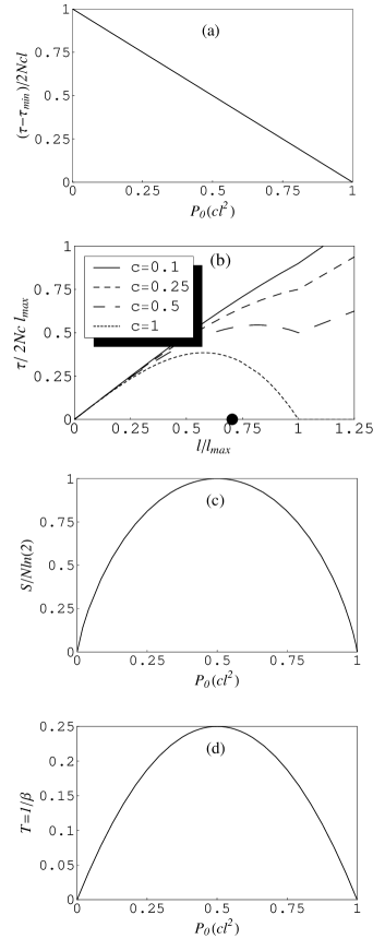
Figure 2: Thermodynamic and mechanical response as a function of imposed deformation for the global-load sharing model: (a) the difference between the average Young’s modulus $\tau/l$ and the minimum Young’s modulus $\tau_{min}/l$ (that holds in the entirely damaged configuration); (b) average stress for a few particular models (the black dot is the percolation critical-point transition); (c) Shannon entropy; and (d) temperature.

Most importantly for our present purposes, since the probabity $P_{0}$ of having a site broken in this model is independent of the configuration and site location, the global load-sharing damage model is exactly equivalent to the percolation model with occupation probability $P_{0}(l)$. There is a critical-point phase transition in this model, when $P_{0}(l_{c})=1/2$, for which $S$ goes through a maximum $S=N\ln 2$. The correlation length diverges then as

$$\xi\sim|P_{0}(l)-1/2|^{-\nu}$$ (50)

with $\nu=4/3$ in dimension $D=2$ Stauffer and Aharony (1994). We have in general

$$P_{0}(l)-P_{0}(l_{c})\sim p(cl_{c}^{2})(l-l_{c})$$ (51)

and thus

$$\xi\sim|l-l_{c}|^{-4/3}.$$ (52)

In pathological cases, special q.d. distributions satisfy $p(cl_{c}^{2})=0$ so that $P_{0}(l)-P_{0}(l_{c})\sim(l-l_{c})^{\alpha}$ with $\alpha\neq 1$. This results in

$$\xi\sim|l-l_{c}|^{-4\alpha/3}.$$ (53)

Note that in Ref.Pride and Toussaint (2002), we have treated this model with $c=1$, which did not change anything to the nature of the transition, but only changed the minimum stiffness associated with the most damaged configuration where $\tau_{min}=2N(1-c)l$, and, consequently, the position or existence of a peak stress in the average mechanical response $\tau(l)$. This is seen in Fig. 2(b): the existence, and the position of a possible peak-stress position relative to the percolation transition (black dot $l/l_{max}=1/\sqrt{2}$), depends on the particular model considered. However, the divergence of the correlation length and the associated critical-point nature of the percolation transition are insensitive to $c$.

The present approach does not allow a direct exploration of the avalanche distributions as the critical point is approached. This is because the probability distribution over configurations was obtained at each elongation $l$ by averaging over all realizations of the quenched disorder. To obtain directly a result on avalanches, on the contrary, correlations between successive elongations should be considered for each realization of the q.d., and the average over q.d. should only be considered afterwards. Our damage model nonetheless behaves as a fiber bundle with GLS for which results about the avalanche distribution have been determined Kloster et al. (1997); Hansen and Hemmer (1994); Hemmer and Hansen (1992). If $c$ is sufficiently large that the average strain/stress curve has a peak at $\tau_{c}$, there is a burst in the number of elements that must break before the system is able to sustain the same global force again. The distribution of the burst size $\Delta$ should thus scale as

$$n(\Delta)\sim\Delta^{-5/2}e^{-\Delta/\Delta_{0}},$$

with $\Delta_{0}\sim|\tau-\tau_{c}|^{-1/2}$. It might be tempting to relate this power-law behavior of the burst distribution to the behavior of cluster numbers in mean-field percolation (on a Bethe lattice or on hypercubes in dimensionality $D\geq 6$). The average number of clusters of size $s$ per lattice site also scales as $n_{p}(\Delta)\sim\Delta^{-5/2}e^{-\Delta/\Delta_{0}}$ in such models where $\Delta_{0}\sim|p-p_{c}|^{-2}$ Stauffer and Aharony (1994). But the fact that both the cluster number distribution at critical percolation threshold and the burst size distribution at peak stress have the same power law exponent of -5/2 might simply be coincidental. These two points (critical percolation threshold and possible peak stress) in general differ, and the exponents characterizing the evolution of the upper cutoff $\Delta_{0}$ of these distributions close to percolation threshold or peak stress seem also unrelated.

V.2 Local load model

In this case, $J_{xy}=\alpha$ when $x,y$ are nearest neighbors, and zero otherwise. Defining the order parameter $\sigma\in\left\{-1,1\right\}$ as $\sigma=2\varphi-1$, we note that

$$\sum_{xy}J_{xy}\varphi_{x}\varphi_{y}=\alpha N+2\alpha\sum_{x}\sigma_{x}+\frac{\alpha}{4}\sum_{<xy>}\sigma_{x}\sigma_{y}$$ (54)

where $<xy>$ denotes a sum on nearest neighbors only. Consequently, the probability over configurations can be cast under the form

$$P[\sigma,l] = e^{\beta(E\sum_{x}\sigma_{x}+J\sum_{<xy>}\sigma_{x}\sigma_{y})}/Z,$$ (55)

which is exactly a classical Ising model with coupling constant and external field given by

$$\beta J = \frac{\alpha p(cl^{2})\varepsilon l^{2}}{4P_{0}(1-P_{0})},$$ (56)

$$\beta E = \frac{1}{2}\ln\left[\frac{P_{0}}{1-P_{0}}\right]+\frac{2\alpha p(cl^{2})\varepsilon l^{2}}{P_{0}}.$$ (57)

The critical point of this model is at Huang (1987)

$$(\beta J_{c},\beta E)=(A_{c},0)$$

with $A_{c}=\ln(1+\sqrt{2})/2$. The external field $\beta E$ starts at infinitely negative values, and ends up at infinitely positive ones. It evolves continuously and thus necessarily crosses $E=0$ at the $l_{c}$ satisfying , from Eq. (57),

$$P_{0}(l_{c})\left\{\ln[1-P_{0}(l_{c})]-\ln[P_{0}(l_{c})]\right\}=4\alpha p(cl_{c}^{2})\varepsilon l_{c}^{2}.$$ (58)

The mean-field percolation result of $P_{0}(l_{c})=1/2$ is thus recovered when the coupling vanishes ($J=0$), which is a consistency check.

More generally, for non-zero nearest coupling constants $\alpha$, the system will undergo a first-order transition if at $l_{c}$ satisfying Eq. (58), the formal inverse temperature satisfies

$${\beta(l_{c})J=\frac{\alpha p(cl_{c}^{2})\varepsilon l_{c}^{2}}{4P_{0}(l_{c})(1-P_{0}(l_{c}))}=}$$ (59)

$$\frac{\ln[1-P_{0}(l_{c})]-\ln[P_{0}(l_{c})]}{16(1-P_{0}(l_{c}))}>A_{c}.$$

Depending on the value of $\beta(l_{c})J$, the system can display four types of behavior, that are schematically depicted in Fig. 3:

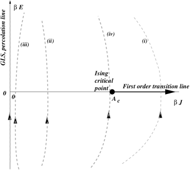
Figure 3: Possible Paths in the space of coupling constants of Ising models, under increasing imposed elongation associated to different Local Load Sharing damage models.

(i) For many q.d. distributions, the first value of $l_{c}$ satisfying Eq. (58) occurs for very small values of $P_{0}(l_{c})$, that correspond to small values of $2\alpha p(cl_{c}^{2})\varepsilon l_{c}^{2}$, since $x\ln[(1-x)/x]\rightarrow 0^{+}$ when $x\rightarrow 0$. In this case, $\ln[(1-P_{0}(l_{c}))/P_{0}(l_{c})]/(1-P_{0}(l_{c}))\simeq-\ln[P_{0}(l_{c})]\geq 1$, and the condition of Eq. (59) is fulfilled. The system thus goes through a first-order phase transition at this $l_{c}$ and there is a discontinuous jump in the average number of broken cells and the average stress (which are related to first derivatives of the free energy with respect to $l$ or $\mu$, and are similar to the average number of spins up in an Ising model) Huang (1987). The correlation length increases up to the transition but remains finite. All of this behavior for such local load models has been documented in the literature Kloster et al. (1997); Hansen and Hemmer (1994); Hidalgo et al. (2002).

However, three other behaviors are also possible if $\beta(l_{c})J<A_{c}$ at the point $l_{c}$ at which the external field vanishes [Eq. (58)]. Whether this occurs is controlled by the type of q.d. distribution and the value of the coupling constant $\alpha$. When $\beta(l_{c})J<A_{c}$, no first order transition is encountered and one can further classify the transition into three subcategories:

(ii) If $\beta(l_{c})$ has a finite value of order unity, significantly below $A_{c}$, the system simply goes continuously through $l_{c}$, without discontinuity in sustained load or average number of cracks. The correlation length remains finite.

(iii) If $\beta(l_{c})J\ll 1$, (which should happen for vanishing $\alpha$), the distribution over configurations is dominated by the external field, and the system essentially behaves as a percolation model going through the percolation transition. Although there should be corrections due to the nonzero character of $\beta(l_{c})J$, these might be smaller than the finite-size corrections in numerical realizations, and the correlation length would then be found to diverge up to the system size as $\xi\sim|l-l_{c}|^{-4/3}$.

(iv) Finally, if $\beta(l_{c})J\sim A_{c}^{-}$, the system comes close to the critical point of the Ising model at $l_{c}$, and the correlation length should diverge corresponding as in an Ising system whose temperature comes close to $1/A_{c}=T_{c}$ from above, while the external field reverts sign. The slope of the average mechanical curve $\tau(l)$ should also locally diverge around $l_{c}$. The exponents associated with the divergence of $\xi$ as function of $(l-l_{c})$ depend on the way the critical point is approached as a function of $l$. For values of $l$ such that $\beta E(l)\ll 1$, we write $1/\beta(l)J\sim T_{c}+f(l)$, and $\xi\sim|T(l)-T_{c}|^{-\nu}=|f(l)|^{-\nu}$ where $\nu=1$ for the 2D Ising model. The correlation length therefore diverges as $|l-l_{c}|^{-\nu}$, unless the temperature has a quadratic minimum in $l$ close to $l_{c}$ in which case it diverges as $|l-l_{c}|^{-2\nu}$.

V.3 Power-law decay

We last consider the general case of stress perturbations decaying as power-laws of the distance to broken cells, $J(x)\sim\alpha(x/d)^{-\gamma}/\Phi(\gamma)$, where $\alpha$ is of order unity, $d$ is the lattice constant, and $\Phi(\gamma)=\sum_{y\neq x}(|y-x|/d)^{-\gamma}$ is a normalizing factor (which depends on the lattice size if $\gamma>D$, where $D$ is the system´s dimension). To be consistent, the models considered here are biperiodic of linear size $L$, and the interactions are put to $0$ for distances above $L$. This type of model, considered for example by Hidalgo et al Hidalgo et al. (2002); Yewande et al. (2003), allows us to span ranges between purely global sharing (when $\gamma=0$), to the local sharing limit ($\gamma\rightarrow\infty$). Equations (42-44) show that this model leads to probability distributions over configurations of the form

$$P[\sigma,l] = e^{\beta(E\sum_{x}\sigma_{x}+\sum_{x\neq y}J(|x-y|)\sigma_{x}\sigma_{y})}/Z,$$ (60)

which is a generalized long-range Ising model with coupling constants and external field given by:

$$\beta J(r) = \frac{\alpha p(cl^{2})\varepsilon l^{2}}{4P_{0}(1-P_{0})}\frac{(r/d)^{-\gamma}}{\Phi(\gamma)},$$ (61)

$$\beta E = \frac{1}{2}\ln(\frac{P_{0}}{1-P_{0}})+\frac{\alpha p(cl^{2})\varepsilon l^{2}}{2P_{0}}.$$ (62)

Note that although the case $\gamma\rightarrow\infty$ is isomorphic to the Local Load Sharing Model introduced in the previous section, the Global Load Sharing Model of Section V.1 corresponds to $\alpha=0$, but not to the exponent $\gamma=0$. The presence of the quadratic coupling makes this later case isomorphic to a Curie-Weiss model, which is the Mean-Field theory of Ising models.

Although such long-range Ising models are still an open area of research, it has been proposed Cannas et al. (2004, 2000); Cannas and Tamarit (1996) that their behavior can be classified into two categories depending on whether $\gamma>D$ or $\gamma<D$. In the short-range case, $\gamma>D$, this model admits a traditional thermodynamic limit when $L\rightarrow\infty$. Although $\Phi(\gamma)$ diverges when $L\rightarrow\infty$, the thermodynamic limit is well defined once $\Phi(\gamma)$ is introduced into the coupling constants $J(r)={(r/d)^{-\gamma}}/{\Phi(\gamma)}$. Thus, the free or internal energy per lattice site, entropy and magnetization all admit a finite limit when $L\rightarrow\infty$, and are functions of $\beta$ and the external field $E$.

In our case, we have

$$\beta = \frac{\alpha p(cl^{2})\varepsilon l^{2}}{4P_{0}(1-P_{0})}$$

$$\beta E = \frac{1}{2}\ln(\frac{P_{0}}{1-P_{0}})+\frac{\alpha p(cl^{2})\varepsilon l^{2}}{2P_{0}}.$$

With $J$ defined as above, the Ising model shows that in the limit $\gamma\rightarrow\infty$, the critical point is at

$$\lim_{\gamma\rightarrow\infty}\beta_{c}=\ln(1+\sqrt{2})/2.$$

It has also been shown Cannas and Tamarit (1996) that as $\gamma\rightarrow D^{+}$, $\beta_{c}\sim 1$. All short-range models $\gamma>D$ display critical points at finite temperature, and since all of them have a finite range of interaction, one can conjecture that all of them belong to the same universality class as the Ising model, with a critical point such that $\beta_{c}$ is of order unity . It has also been conjectured that all nonlocal models $\gamma<D$ belong to the Curie-Weiss universality class of the Mean Field Ising model. They also present critical temperatures such that $\beta_{c}$ is of order one Cannas et al. (2000). The Curie-Weiss model corresponds to the mean-field coupling $J_{xy}=1/N$, independently of $x$ and $y$, where $N$ is total number of cells in the system. For the Curie-Weiss model, the p.d.f. over state configurations is $P[\sigma]\propto\exp[\beta(E\sum_{x}\sigma_{x}+\sum_{xy}\sigma_{x}\sigma_{y}/N)]\propto\exp[\beta(E\sum_{x}\sigma_{x}+(\sum_{x}\sigma_{x})^{2}/2N)]$.

All this suggests the following classifications of our damage models:

(1) If the coupling constant is small ($\alpha\ll 1$), the damage model is close to the percolation model so that in the approach to the transition at elongation $l_{c}$, the correlation length behaves as $\xi\sim|l-l_{c}|^{-\nu}$, with $\nu=4/3$;

(2) For non-negligeable coupling constants $\alpha$, in the short-range case $\gamma>D$, we recover the same three possible behaviors as described above for the local load sharing rule;

(3) In the long-range case where $\gamma<D$, we again recover the same type of four scenarios depending on the ratio $\beta(l_{c})/A_{c}$ (as discussed in the local-load sharing case). The model behaves as percolation when $\alpha\ll 1$. Otherwise, the behavior is determined by the ratio $\beta(l_{c})/A_{c}$. Note that $A_{c}$ is of order unity, but depends on the particular exponent $\gamma$ and on the system size. If $\beta(l_{c})/A_{c}<1$, the system behaves continuously and no transition is observed. If $\beta(l_{c})/A_{c}>1$, there is a discrete jump in both the average number of broken cells and the sustained load. The correlation length remains finite in both of these two cases. Only the limiting case of $\beta(l_{c})/A_{c}\sim 1$ corresponds to a second-order phase transition. In any of these cases, for large enough systems, the Curie-Weiss description holds according to Refs. Cannas et al. (2004, 2000); Cannas and Tamarit (1996). Accordingly, if there is any divergence of correlation length due to the system coming close to $\beta(l_{c})/A_{c}\sim 1$ at $E=0$, the associated exponents should be those of the Curie-Weiss mean-field critical point ($\nu=1/2$), and not the Ising one.

These results can be compared to numerical-simulation results in the literature for related models. In fiber bundle models with power-law interactions Hidalgo et al. (2002), a transition has been found as a function of the interaction exponent $\gamma$ that is consistent with the above analysis, predicting mean-field behavior for the long-range case $\gamma<D$, and Ising-like behavior in the short-range case $\gamma>D$. Typical configurations prior to breakdown for this type of system are displayed in Fig. 5 of Ref. Hidalgo et al. (2002), and look very similar to percolation configurations close to the transition in the case $\gamma=0$, displaying shorter and shorter cluster sizes (characteristic of the autocorrelation length) and compact configurations as $\gamma$ increases above $D$. This is coherent with a mean-field behavior close to percolation transition in the first case, as opposed to a first order transition (analogous to Ising model crossing $E=0$ below $T_{c}$) when $\gamma<D$. This analogy is even more apparent in Fig. 7, bottom, of Ref. Yewande et al. (2003), where an extension of this model was considered, with time-delayed fiber breaking process in addition to this power-law decaying interactions Yewande et al. (2003).

Burned fuse models, in which the interactions between burned fuses decay as $1/r^{D}$, exhibit diverging autocorrelation lengths at breakdown, with $\xi\sim|l-l_{c}|^{-\nu}$ where $l$ is the imposed voltage, and $\nu$ is equal to the percolation exponent Stauffer and Aharony (1994), $\nu=4/3$ in 2D Hansen and Schmittbuhl (2003) or $0.88$ in 3D Ramstad et al. (2004). The morphology of the connected “fracture” at breakdown is oriented, and different from percolating clusters in the percolation model. This seems to be related to the anisotropic character of interactions in the burned-fuse model; i.e., the current perturbation from a burned fuse goes as a dipolar field decaying as $1/r^{D}$, but also having an orientational aspect not included in the models under study in this paper. Based on this, Hansen et al. Hansen and Schmittbuhl (2003) relate the roughness of the spanning fracture to the autocorrelation length exponent, based on arguments of percolation in gradient, and this properly predicts the Hurst exponent of the final damage fronts, both in 2 and 3D. This anisotropic aspect is absent from the models discussed here, but the fact that the autocorrelation length exponent is similar to the ones of percolation, is coherent with the fact that long-range systems are in the percolation universality class. Burned fuse systems are at the verge between short and long range interactions, in the sense that they correspond to $\gamma=D$.

Last, fiber bundles connected to elastic plates, where $\gamma=1$ and $D=2$, have been numerically studied in Ref. Schmittbuhl et al. (2003) and an autocorrelation length exponent of $\nu\simeq 1.54$ numerically determined. The present theory does not explain this autocorrelation exponent. The discrepancy between this result and the percolation or Curie-Weiss critical point result, might presumably result from finite-size effects making this model ($\gamma=1$) still significantly different from the Curie Weiss one ($\gamma=0$), or from the fact that the stress perturbation was in this numerical model too large for the small perturbation expansion performed here to apply.

VI Conclusions

We have treated a class of damage models having weak isotropic interactions between cells that become damaged in the lattice. A quenched disorder is present in the rupture energies for each lattice cell, and the evolution of damage is ruled by the Griffith principle. Averaging over all possible realizations of the underlying quenched disorder, the probability distribution of each possible damage configuration was obtained as a function of the deformation externally applied to the system.

The exact calculation is analytically tractable in the case of a global load sharing model, and it has been shown to be isomorphic to a percolation model. This corresponds to the behavior of a system totally dominated by the underlying disorder, where the next cell to break is always the weakest one. Spatial interactions added to the system modify this picture, since the overload created by broken cells induce some degree of spatial ordering that competes with the weakest-cell mechanism. By limiting ourselves to small overloads compared to the average load of the system, it was possible to obtain the probability of damage configurations as integrated over all realizations of the quenched disorder.

In this weak interaction limit, the resulting probability distributions were shown to be Boltzmannians in the number of broken cells and in the stored elastic energy. This type of distribution maximizes Shannon´s entropy under constraints related to the energetic balance of the fracture process, and we have demonstrated the formal relationship between our quenched-disorder damage models and the standard distributions arising in equilibrium statistical mechanics. This then allows the standard toolbox of statistical mechanics to be applied to our damage models.

Our systems map onto three types of possible behaviors: (1) percolation models in the case of interactions so weak, they may be neglected; (2) Ising models for non-negligeable short-range interactions; and (3) Curie-Weiss mean-field theory for non-negligeable long-range interactions. The temperature and external field in the partition function of our models are analytical functions that depend on the particular sharing rule, on the type of quenched disorder considered, and on the average elongation (or deformation) externally loaded onto the system. The path followed in the Ising control parameter space when the load is increased from $0$ depends on the q.d. distribution and the load-sharing rule. When the formal external field reverts sign, a phase transition is possible. This can correspond to a first-order phase transition, a percolation-like transition, or an Ising critical-point transition, depending on the value of the formal temperature during the transition.

The systems studied here are limited to isotropic load perturbations. We have earlier studied oriented crack models in Toussaint and Pride (2002a, b, c), which corresponds to anisotropic load perturbations that depend on the orinetation of the crack opened in the lattice. Those earlier studies were based on an entropy-maximum assumption. The hypotheses of the present work extend directly to oriented systems, and so the present paper justifies the entropy-maximum assumption postulated in our earlier work. The precise value of the temperature, and the physical interpretation of the functional forms given in Toussaint and Pride (2002a, b, c), should be modified according to the results of this paper. Such modifications will, however, result in identical functional forms relating the configuration space and the p.d.f. over configurations, and thus the present work confirms the existence of a phase transition in such an oriented crack model, with an associated divergence exponent of the autocorrelation length, $\nu=2$.

Appendix A Recoverable Energy as a Function of the Damage State

The argument here will be specific to a fiber bundle model. However, as noted in the text, other weak damage models will also be controlled by the same type of stored-energy function obtained here.

Define a fiber bundle as (initially) $N$ fibers stretched between a free rigid plate and an elastic half-space. The rigid plate has a controlled displacement $l$ applied to it that stretches the fibers and the elastic half-space. As a fiber breaks at fixed $l$, the force it held will be transmitted to the other fibers through the elastic half-space.

A fiber at point x is stretched a distance $\ell_{\textbf{x}}$. Where that fiber is attached to the elastic halfspace, the surface of the halfspace displaces an amount $u_{\textbf{x}}$. Thus, at those places x where fibers exist, we have

$$l=\ell_{\textbf{x}}+u_{\textbf{x}}.$$ (63)

The fiber at point x exerts a force on the elastic half-space that is

$$\frac{f_{\textbf{x}}}{A_{F}}=Y_{F}(1-\varphi_{\textbf{x}})\frac{\ell_{\textbf{x}}}{L_{F}}$$ (64)

where $A_{f}$ is the x-sectional area of the fiber (assumed to be independent of the extension), $L_{F}$ is the inital length of each fiber, and $Y_{F}$ is the Young’s modulus of each fiber. The local order parameter $\varphi_{\textbf{x}}$ is 0 if the fiber is intact and 1 if broken.

The Green function for point forces acting on the surface of an elastic halfspace Landau and Lifshitz (1986) yields

$$u_{\textbf{x}}=u_{3}({\textbf{x}}) = \frac{1-\sigma_{s}^{2}}{\pi Y_{s}}\sum_{{\textbf{y}}\neq{\textbf{x}}}\frac{f_{\textbf{y}}}{|{\textbf{y}}-{\textbf{x}}|}$$ (65)

$$= \frac{1-\sigma_{s}^{2}}{\pi}\frac{Y_{F}}{Y_{s}}\frac{A_{F}}{L_{F}}\sum_{{\textbf{y}}\neq{\textbf{x}}}\frac{(1-\varphi_{\textbf{y}})}{|{\textbf{y}}-{\textbf{x}}|}\ell_{\textbf{y}}$$ (66)

where $Y_{s}$ is the Young’s modulus and $\sigma_{s}$ the Poisson’s ratio of the elastic solid. In general, the displacement at a point ${\textbf{x}}=(x_{1},x_{2},x_{3})$ within the elastic solid (where $x_{3}=0$ defines the surface) due to a point force acting at a point ${\textbf{y}}=(y_{1},y_{2},0)$ on the surface [i.e., ${\textbf{f}}({\textbf{x}})=f_{\textbf{y}}\delta({\textbf{x}}-{\textbf{y}})\hat{\textbf{3}}$] is given by

$$\mbox{\hskip-14.22636pt}u_{1} \!\!\!=\!\!\! \frac{1+\sigma_{s}}{2\pi Y_{s}}\left[\frac{(x_{1}-y_{1})x_{3}}{r^{3}}-\frac{(1-2\sigma_{s})(x_{1}-y_{1})}{r(r+x_{3})}\right]f_{\textbf{y}}$$ (67)

$$\mbox{\hskip-14.22636pt}u_{2} \!\!\!=\!\!\! \frac{1+\sigma_{s}}{2\pi Y_{s}}\left[\frac{(x_{2}-y_{2})x_{3}}{r^{3}}-\frac{(1-2\sigma_{s})(x_{2}-y_{2})}{r(r+x_{3})}\right]f_{\textbf{y}}$$ (68)

$$\mbox{\hskip-14.22636pt}u_{3} \!\!\!=\!\!\! \frac{1+\sigma_{s}}{2\pi Y_{s}}\left[\frac{x_{3}^{2}}{r^{3}}+\frac{2(1-\sigma_{s})}{r}\right]f_{\textbf{y}}$$ (69)

where

$$r=\left[(x_{1}-y_{1})^{2}+(x_{2}-y_{2})^{2}+x_{3}^{2}\right]^{1/2}.$$ (70)

Putting $x_{3}=0$ in the expression for $u_{3}({\textbf{x}};{\textbf{y}})$ and then summing over all y yields the expression for the displacement $u_{\textbf{x}}$ of the surface.

We now define the dimensionless number

$$\varepsilon=\frac{(1-\sigma_{s}^{2})}{\pi}\frac{Y_{F}}{Y_{s}}\frac{A_{F}}{L_{F}L_{P}},$$ (71)

where a length $L_{P}$ has been defined as

$$\frac{1}{L_{P}}=\sum_{\bf y\neq\bf x}\frac{1}{|{\bf y-\bf x}|};$$ (72)

i.e., this sum is independent of which point ${\bf x}$ is considered. Assuming either that the elastic halfspace is stiffer than the fibers, or that each fiber has a length much great than its width, or that fibers are spaced far enough apart that $L_{p}$ is large, allows $\varepsilon$ to be considered a small number. Since the fiber bundle is assumed to be made of a finite number $N$ of fibers, there is no divergence to $L_{P}$.

Using these definitions along with $u_{\textbf{x}}=l-\ell_{\bf x}$ and iterating Eq. (66) once to get the leading order in $\varepsilon$ contribution gives

$$\frac{\ell_{\bf x}}{l}=1+\varepsilon\left(-1+\sum_{\bf y\neq\bf x}\frac{L_{P}}{|{\bf y-\bf x}|}\varphi_{\bf y}\right)+O(\varepsilon^{2}).$$ (73)

The elastic strain energy reversibly stored in each surviving fiber is then

$$\mbox{\hskip-17.07164pt}E_{\bf x} = \frac{1}{2}f_{\bf x}\ell_{\bf x}=\frac{1}{2}\frac{A_{F}Y_{F}}{L_{F}}l^{2}(1-\varphi_{\bf x})\left(\frac{\ell_{\bf x}}{l}\right)^{2}$$ (75)

$$= \frac{1}{2}\frac{A_{F}Y_{F}}{L_{F}}l^{2}\left\{1-\varphi_{\bf x}\phantom{\sum_{x}^{y}\left[\frac{L^{2}}{L^{2}}\right]}\right.$$

$$\left.+2\varepsilon\!\left[-1+\varphi_{\bf x}+\sum_{\bf y\neq\bf x}\frac{L_{P}}{|{\bf y-\bf x}|}\varphi_{\bf y}(1-\varphi_{\bf x})\right]\!\right\}.$$

where terms of $O(\varepsilon^{2})$ have been dropped. Thus, upon summing over all the fibers we obtain the total energy $E_{F}$ stored in the fibers as a function of the damage state

$$\mbox{\hskip-25.60747pt}E_{F}=\sum_{\bf x}E_{\bf x}=\frac{1}{2}\frac{A_{F}Y_{F}}{L_{F}}l^{2}$$

$$\mbox{\hskip-25.60747pt}\times\!\left[(1-2\varepsilon)N-(1-4\varepsilon)\!\sum_{\bf x}\!\varphi_{\bf x}-\varepsilon\!\!\!\sum_{{\bf x},{\bf y}\neq{\bf x}}\!\!\!J_{\bf x\bf y}\varphi_{\bf x}\varphi_{\bf y}\right]$$ (76)

where the coupling constant is defined

$$J_{\bf x\bf y}=\frac{2L_{P}}{|{\bf y-\bf x}|}.$$ (77)

This form of the fiber energy is consistent with what was defined in the text.

We now demonstrate that the energy recoverably stored in the elastic solid makes no important modification to $E_{F}$. The strain energy in the solid is given by

$$E_{s}=\frac{Y_{s}}{2(1+\sigma_{s})}\int_{x_{3}>0}d^{3}{\bf x}\sum_{\bf y\neq\bf x}\left(e_{ik}e_{ik}+\frac{\sigma_{s}}{1-2\sigma_{s}}e_{ll}^{2}\right)$$ (78)

where summation over the indices is assumed and where the strain tensor is defined

$$e_{ik}({\textbf{x}};{\textbf{y}})=\frac{1}{2}\left(\frac{\partial u_{i}({\textbf{x}};{\textbf{y}})}{\partial x_{k}}+\frac{\partial u_{k}({\textbf{x}};{\textbf{y}})}{\partial x_{i}}\right).$$ (79)

The displacements are given by Eqs. (67)–(69).

From these equations, the strain at points ${\bf x}$ inside the elastic solid takes the leading-order in $\varepsilon$ form

$$e_{ik}=\varepsilon lL_{P}\left[c_{ik}+\varepsilon\sum_{\bf y\neq\bf x}\frac{f_{ik}({\bf x-\bf y})}{|{\bf x-\bf y}|^{2}}\varphi_{\bf y}\right]$$ (80)

where the constant tensor $c_{ik}$ has units of inverse-length squared and the average strain tensor throughout the elastic solid is $\varepsilon lL_{P}c_{ik}$. The perturbation term due to broken fibers volume integrates to zero. The tensor $f_{ik}$ has no dependence on the norm $|{\bf x-\bf y}|$; however, this fact is immaterial since $f_{ik}$ plays no important role.

Upon forming the required products for the integrand in Eq. (78), and using the fact that terms linear in the broken-fiber perturbations integrate to zero, one obtains that the energy stored in the elastic solid is

$$E_{s}=\frac{1}{2}\frac{A_{F}Y_{F}}{L_{F}}l^{2}\varepsilon VL_{p}\left(c_{ik}c_{ik}+\frac{\sigma_{s}}{1-2\sigma_{s}}c_{ll}^{2}\right)\left[1+O(\varepsilon^{2})\right]$$ (81)

where $V$ is the volume integrated over (assumed finite). In otherwords, any energy stored in the elastic solid that is due to the interaction between fibers, is $\varepsilon^{2}$ smaller than the leading-order contribution which itself can be considered small. The leading order contribution only depends on the average number of broken fibers and thus does not alter the analytical form of Eq. (76). Thus, the energy stored in the elastic solid plays no essential role in the damage model.

References

- Griffith (1920) A. A. Griffith, Philos. Trans. Roy. Soc. London A 221, 163 (1920).
- Herrmann and Roux (1990) H. J. Herrmann and S. Roux, eds., Statistical models for the fracture of disordered media (North-Holland, Amsterdam, 1990).
- Daniels (1945) H. E. Daniels, Proc. R. Soc. A 183, 404 (1945).
- Daniels (1989) H. E. Daniels, Adv. Appl. Probab. 21, 315 (1989).
- Coleman (1958) B. D. Coleman, J. Appl. Phys. 29, 968 (1958).
- Peirce (1926) F. T. Peirce, J. Text. Ind. 17, 355 (1926).
- Sornette (1989) D. Sornette, J. Phys. A 22, L243 (1989).
- Sornette (1992) D. Sornette, J. Phys. I France 2, 2089 (1992).
- Andersen et al. (1997) J. V. Andersen, D. Sornette, and K. W. Leung, Phys. Rev. Lett. 78, 2140 (1997).
- Hemmer and Hansen (1992) P. C. Hemmer and A. Hansen, J. Appl. Mech. 59, 909 (1992).
- Pride and Toussaint (2002) S. R. Pride and R. Toussaint, Physica A 312, 159 (2002).
- Hansen and Hemmer (1994) A. Hansen and P. C. Hemmer, Phys. Lett. A 184, 394 (1994).
- Kloster et al. (1997) M. Kloster, A. Hansen, and P. C. Hemmer, Phys. Rev. E 56, 2615 (1997).
- Zhang and Ding (1996) S. D. Zhang and E. J. Ding, Phys. Rev. B 53, 646 (1996).
- Hidalgo et al. (2002) R. C. Hidalgo, Y. Moreno, F. Kun, and H. J. Herrmann, Phys. Rev. E 65, 046148 (2002).
- Yewande et al. (2003) O. E. Yewande, Y. Moreno, F. Kun, R. C. Hidalgo, and H. J. Herrmann, Phys. Rev. E 68, 026116 (2003).
- Bakke et al. (2003) J. O. H. Bakke, J. Bjelland, T. Ramstad, T. Stranden, A. Hansen, and J. Schmittbuhl, Phys. Scripta A T106, 65 (2003).
- Batrouni and Hansen (1998) G. G. Batrouni and A. Hansen, Phys. Rev. Lett. 80, 325 (1998).
- De Arcangelis and Herrmann (1989) L. De Arcangelis and H. J. Herrmann, Phys. Rev. B 39, 2678 (1989).
- De Arcangelis et al. (1989) L. De Arcangelis, A. Hansen, H. J. Herrmann, and S. Roux, Phys. Rev. B 40, 877 (1989).
- Duxbury et al. (1987) P. M. Duxbury, P. L. Leath, and P. D. Beale, Phys. Rev. B 36, 367 (1987).
- Hansen and Schmittbuhl (2003) A. Hansen and J. Schmittbuhl, Phys. Rev. Lett. 90, 045504 (2003).
- Hansen et al. (1991) A. Hansen, E. L. Hinrichsen, and S. Roux, Phys. Rev. B 43, 665 (1991).
- Zapperi et al. (2000) S. Zapperi, H. J. Herrmann, and S. Roux, Eur. Phys. J. B 17, 131 (2000).
- Zapperi et al. (2003) S. Zapperi, H. J. Herrmann, and S. Roux, Fractals 11, 327 (2003).
- Batrouni et al. (2002) G. G. Batrouni, A. Hansen, and J. Schmittbuhl, Phys. Rev. E 65, 036126 (2002).
- Herrmann et al. (1989) H. J. Herrmann, A. Hansen, and S. Roux, Phys. Rev. B 39, 637 (1989).
- Schmittbuhl et al. (2003) J. Schmittbuhl, A. Hansen, and G. G. Batrouni, Phys. Rev. Lett. 90, 045505 (2003).
- Bouchaud (1997) E. Bouchaud, J. Phys. Condens. Matt. 9, 4319 (1997).
- Schmittbuhl et al. (1995) J. Schmittbuhl, F. Schmitt, and C. H. J. Scholz, J. Geophys. Res. B 100, 5953 (1995).
- Schmittbuhl et al. (1993) J. Schmittbuhl, S. Gentier, and S. Roux, Geophys. Res. Lett. 20, 639 (1993).
- Lea Cox and Wang (1993) B. Lea Cox and J. S. Y. Wang, Fractals 1, 87 (1993).
- Måløy et al. (1992) K. J. Måløy, A. Hansen, E. L. Hinrichsen, and S. Roux, Phys. Rev. Lett. 68, 213 (1992).
- Bouchaud et al. (1990) E. Bouchaud, G. Lapasset, and J. Planès, Europhys. Lett. 13, 73 (1990).
- Daguier et al. (1996) P. Daguier, S. Henaux, E. Bouchaud, and F. Creuzet, Phys. Rev. E 53, 5637 (1996).
- Daguier et al. (1997) P. Daguier, B. Nghiem, E. Bouchaud, and F. Creuzet, Phys. Rev. Lett. 78, 1062 (1997).
- Schmittbuhl and Måløy (1997) J. Schmittbuhl and K. J. Måløy, Phys. Rev. Lett. 78, 3888 (1997).
- Delaplace et al. (1999) A. Delaplace, J. Schmittbuhl, and K. J. Måløy, Phys. Rev. E 60, 1337 (1999).
- Sapoval et al. (1985) B. Sapoval, M. Rosso, and J. F. Gouyet, J. Phys. (Paris), Lett. 46, L149 (1985).
- Moreno et al. (2001) Y. Moreno, J. B. Gomez, and A. F. Pacheco, Physica A 296, 9 (2001).
- Moreno et al. (2000) Y. Moreno, J. B. Gómez, and A. F. Pacheco, Phys. Rev. Lett. 85, 2865 (2000).
- Zapperi et al. (1997a) S. Zapperi, P. Ray, H. Stanley, and A. Vespignani, Phys. Rev. Lett. 78, 1408 (1997a).
- Zapperi et al. (1999) S. Zapperi, P. Ray, H. Stanley, and A. Vespignani, Phys. Rev. E 59(5), 5049 (1999).
- Zapperi et al. (1997b) S. Zapperi, A. Vespignani, and H. E. Stanley, Nature 388, 658 (1997b).
- Kun et al. (2000) F. Kun, S. Zapperi, and H. J. Herrmann, Eur. Phys. J B 17, 269 (2000).
- Sornette and Andersen (1998) D. Sornette and J. V. Andersen, Eur. Phys. J. B. 1, 353 (1998).
- Caldarelli et al. (1996) G. Caldarelli, F. D. Di Tolla, and A. Petri, Phys. Rev. Lett. 77, 2503 (1996).
- Räisänen et al. (1998) V. I. Räisänen, M. J. Alava, and R. M. Nieminen, Phys. Rev. B 58, 14288 (1998).
- Rundle and Klein (1989) J. B. Rundle and W. Klein, Phys. Rev. Lett. 63, 171 (1989).
- Toussaint and Pride (2002a) R. Toussaint and S. R. Pride, Phys. Rev. E 66, 036135 (2002a).
- Toussaint and Pride (2002b) R. Toussaint and S. R. Pride, Phys. Rev. E 66, 036136 (2002b).
- Toussaint and Pride (2002c) R. Toussaint and S. R. Pride, Phys. Rev. E 66, 036137 (2002c).
- Blumberg Selinger et al. (1991) R. L. Blumberg Selinger, Z. G. Wang, W. M. Gelbart, and A. Ben-Shaul, Phys. Rev. A 43, 4396 (1991).
- Pomeau (1992) Y. Pomeau, C. R. Acad. Sci., Ser. II 314, 553 (1992).
- Roux (2000) S. Roux, Phys. Rev. E 62, 6164 (2000).
- Politi et al. (2002) A. Politi, S. Ciliberto, and R. Scorretti, Phys. Rev. E 66, 026107 (2002).
- Santucci et al. (2003) S. Santucci, L. Vanel, A. Guarino, R. Scorretti, and S. Ciliberto, Europhys. Lett. 62, 320 (2003).
- Ciliberto et al. (2001) S. Ciliberto, A. Guarino, and R. Scorretti, Physica D 158, 83 (2001).
- Guarino et al. (2002) A. Guarino, S. Ciliberto, A. Garcimartin, M. Zei, and R. Scorretti, Eur. Phys. J. B 26, 141 (2002).
- Guarino et al. (1998) A. Guarino, A. Garcimartin, and S. Ciliberto, Eur. Phys. J. B 6, 13 (1998).
- Garcimartin et al. (1997) A. Garcimartin, A. Guarino, L. Bellon, and S. Ciliberto, Phys. Rev. Lett. 79, 3202 (1997).
- Shannon (1948) C. E. Shannon, Bell Systems Technical Journal 27, 373 (1948).
- Stauffer and Aharony (1994) D. Stauffer and A. Aharony, Introduction to percolation theory (Taylor and Francis, London, 1994), 2nd ed.
- Huang (1987) K. Huang, Statistical mechanics (Wiley, N.Y., 1987), 2nd ed.
- Cannas et al. (2004) S. A. Cannas, P. M. Gleiser, and F. A. Tamarit, Recent Research Developments in Physics (Transworld Research Network, 2004), chap. Two dimensional Ising model with long-range competing interactions, to appear, preprint on http://tero.fis.uncor.edu/ cannas/papers/bookchapter3.pdf.
- Cannas et al. (2000) S. A. Cannas, A. C. N. Magalhaes, and F. A. Tamarit, Phys. Rev. B 61, 11521 (2000).
- Cannas and Tamarit (1996) S. A. Cannas and F. A. Tamarit, Phys. Rev. B 54, 12661 (1996).
- Ramstad et al. (2004) T. Ramstad, J. Ø. H. Bakke, J. Bjelland, T. Stranden, and A. Hansen, cond-mat/0311606 (2004), preprint.
- Landau and Lifshitz (1986) L. D. Landau and E. M. Lifshitz, Theory of Elasticity (Pergamon Press, New York, 1986), 3rd ed.