Disordered and Ordered States in a Frustrated Anisotropic Heisenberg Hamiltonian

Abstract

We use a recently proposed perturbative numerical renormalization group algorithm to investigate ground-state properties of a frustrated three dimensional Heisenberg model on an anisotropic lattice. We analyze the ground state energy, the finite size spin gap and the static magnetic structure factor. We find in two dimensions a frustration-induced gapless spin liquid state which separates two magnetically ordered phases. In the spin liquid state, the magnetic structure factor shows evidence that this state is made of nearly disconnected chains. This spin liquid state is unstable against unfrustrated interplane couplings.

Low dimensional quantum magnets are currently the object of an important interest review . This stems from the rich physics which is displayed by these sytems due to their reduced dimension and competing interactions which often push the transition to ordered states to very low temperatures or even preclude the onset of magnetism at all. Geometric frustration is one of the effects which are believed to lead to possible non-classical states. A non-classical ground state exists in a pure one-dimensional quantum antiferromagnet. The ground state is disordered and the low energy excitations are spinons which carry fractional quantum numbers. A fundamental question is whether spinons can survive in higher dimension.

The relevance of these questions has been substantiated in a recent neutron scattering experiment coldea reported in the quantum magnet Cs₂CuCl₄. This compound is a quasi-two dimensional spin one-half Heisenberg antiferromagnet. It is made of anisotropic triangular planes (with $J^{\prime}=J"\approx 0.34J$ in Eq(1)) which are weakly-coupled by an exchange which is roughly $J_{z}=0.045J$. An incommensurate Néel state is stable below $T_{N}=0.62K$ at zero magnetic field. In the two dimensional regime above $T_{N}$, the dynamic correlation displays a highly dispersive continuum of excited states which is a signature of spinons. This finding together with the fact that $J^{\prime}$ is in the same order as $J$ led to the conclusion that above $T_{N}$, Cs₂CuCl₄ is a 2D spin liquid with fractional excitations.

In order to study these effects of frustration and dimensional crossover, we will consider the following anisotropic 3D Heisenberg Hamiltonian:

$$H=J\sum_{i,l,k}{\bf S}_{i,l,k}{\bf S}_{i+1,l,k}+J^{\prime}\sum_{i,l}{\bf S}_{i,l,k}{\bf S}_{i,l+1,k}+$$

$$J"\sum_{i,l,k}{\bf S}_{i,l,k}{\bf S}_{i+1,l+1,k}+J_{z}\sum_{i,l,k}{\bf S}_{i,l,k}{\bf S}_{i,l,k+1},$$ (1)

where the $i$ index represents sites, the $l$ index chains and the $k$ index planes, the exchange couplings are such that $J_{z}\ll J=1$ and $J^{\prime},J"\lesssim 1$. When $J^{\prime}\neq 0$ and $J"\neq 0$ the system is frustrated. In this case the Quantum Monte Carlo method, which is so far the most reliable method of investigation of spin systems, is plagued by the sign problem. Alternative approaches series ; RPA have investigated the possibility of a spin liquid state in the 2D regime ($J_{z}=0$) of the Hamiltonian(1). In Ref. series , this 2D model was studied using a combination of Ising and dimer series expansions. Considering the extrapolation of their results to the limit of weakly coupled chains, the authors was not able to conclude clearly due to the limitation of their technique. They argued that either a spiral ordered or a nearly critical disordered phase are possible in this regime. The dynamical susceptibility of this model was computed within the Random Phase Approximation (RPA) RPA using an essentially exact expression for the 1D chain dynamical susceptibility. For the 2D system incommensurate order with exponentially small characteristic wave vector is predicted. But this prediction was inspired by the experimental observation. It is impossible to tell from this study if this is an intrinsic behavior of the Hamiltonian(1).

We wish to present in this letter an ab-initio computation of the ground state static properties of the Hamiltonian(1). For this purpose, we use a recently proposed perturbative density matrix renormalization group (DMRG) approach moukouri-TSDMRG ; moukouri-TSDMRG2 ; moukouri-KB ; alvarez-ED . This perturbative DMRG method which has been so far used for only anisotropic 2D systems is extended here to anisotropic 3D systems. We will explore the following issues: (i) what is the nature of the ground state in the 2D regime of the Hamiltonian (1)? (ii) Is a spin liquid state favored when $J^{\prime}=J"=0.3$ as found experimentally? If so, what is the nature of this spin liquid state? (iii) Does $J_{z}$ restore a magnetic state starting from this eventual spin liquid state? If so, is this order incommensurate?

The perturbative DMRG which will be used in this study is a particular case of a more general matrix perturbation method based on Kato-Bloch expansion kato ; bloch which was recently introduced by one of us moukouri-KB . In the first step, the usual 1D DMRG method white is applied to find a set of low lying eigenvalues $\epsilon_{n}$ and eigenfunctions $|\phi_{n}\rangle$ of a single chain. One can note that during this step, if one wishes to study not too large lattices, it is preferable to use the exact diagonalization method instead of the DMRG. The advantage of the exact diagonalization method is that by selecting both the total spin $S$ and the momentum in addition to the $S_{z}$ component of $S$ as done in DMRG, it will lead to a better estimation of the low energy Hamiltonian of a single chain.

In the second step, the 2D Hamiltonian (Eq.(1) with $J_{z}=0$ )is then projected onto the basis constructed from the tensor product of the $|\phi_{n}\rangle$’s. This projection yields an effective one-dimensional Hamiltonian for a single plane (we drop temporaly the plane index $k$),

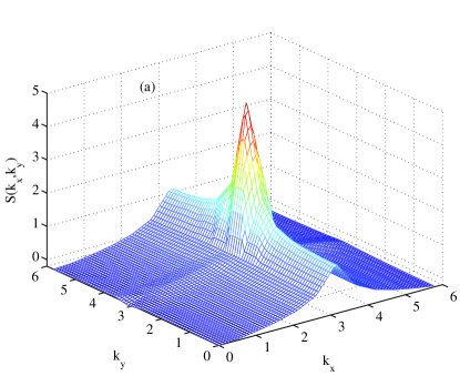
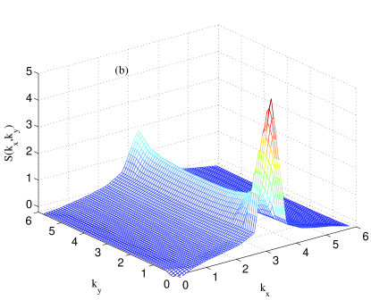
Figure 1: Static spin structure factor $S(k_{x},k_{y})$ for $L_{x}\times L_{y}=24\times 25$, $J^{\prime}=0.3$, $J"=0$ (upper graph) and $J^{\prime}=0.3$, $J"=0.6$ (lower graph)

$$\tilde{H}_{2}\approx\sum_{[n]}E_{[n]}|\Phi_{[n]}\rangle\langle\Phi_{[n]}|+J^{\prime}\sum_{l}{\bf\tilde{S}}_{l}{\bf\tilde{S}}_{l+1}+$$

$$J"\sum_{l}{\bf\tilde{S}}_{l}{\bf\tilde{S}}_{l+1}$$ (2)

where $E_{[n]}$ is the sum of eigenvalues of the different chains, $E_{[n]}=\sum{\epsilon_{n_{l}}}$; $|\Phi_{[n]}\rangle$ is the corresponding eigenstate, $|\Phi_{[n]}\rangle=|\phi_{n_{1}}\rangle|\phi_{n_{2}}\rangle...|\phi_{n_{L}}\rangle$; the composite chain-spin operators on the chain $l$ are ${\bf\tilde{S}}_{l}=({\bf\tilde{S}}_{1l},{\bf\tilde{S}}_{2l},...{\bf\tilde{S}}_{Ll})$, where the running index labels sites in a chain $l$. Note that the products of spin-chain operators in Eq. 2 are different for the terms involving $J^{\prime}$ and $J"$. The term with $J^{\prime}$ couples spins with same site index on neighboring chains, when the one with $J"$ couples spins with site index $i$ on chain $l$ and $i-1$ on chain $l+1$ are coupled. These renormalized matrix elements on the single chain basis are

$${\bf\tilde{S}}_{i,l}^{n_{l},m_{l}}=\langle\phi_{n_{l}}|{\bf S}_{i,l}|\phi_{m_{l}}\rangle$$ (3)

The effective Hamiltonian (2) is one-dimensional and it is also studied by the DMRG method. The only difference with a normal 1D situation is that the local operators are now $m\times m$ matrices, where $m$ is the number of states kept to describe the single chain.

In the third step, the same procedure is repeated in order to go from 2D to 3D once $J_{z}$ is set on. One then obtains the following effective 1D Hamiltonian for the 3D system:

$$\tilde{H}_{3}\approx\sum_{[p]}E_{[p]}^{\prime}|\Psi_{[p]}\rangle\langle\Psi_{[p]}|+J_{z}\sum_{k}{\bf\tilde{S^{\prime}}}_{k}{\bf\tilde{S^{\prime}}}_{k+1}$$ (4)

where $E_{[p]}^{\prime}$ are the sum of eigenvalues of the decoupled planes, $|\Psi_{[p]}\rangle$ are the corresponding eigenstate, and the composite plane-spin operators on a plane $k$ are ${\bf\tilde{S^{\prime}}}_{k}=({\bf\tilde{S}}_{1k},{\bf\tilde{S}}_{2k},...{\bf\tilde{S}}_{Pk})$, the running index labels chains in a plane $k$. The generation of the effective Hamiltonian (4) is identical to that of the effective Hamiltonian (2) described in Refs.moukouri-TSDMRG ; moukouri-TSDMRG2 . We target the spin sectors $S_{z}=0$, $\pm 1$, and $\pm 2$ to generate a low energy Hamiltonian which describes the 2D systems. In Refmoukouri-TSDMRG2 ; alvarez-ED , this perturbative DMRG was tested against the stochastic series expansion quantum Monte Carlo (QMC) and exact diagonalization methods respectively. The agreement was very good for small transverse couplings and not too large lattices. These comparisons showed that the method is well controlled and its accuracy can systematically be improved by increasing the number of states kept during each step.

We first set $J_{z}=0$ and study the ground state properties of a single plane. We studied lattice sizes ranging from $8\times 9$ to $32\times 33$ for $J^{\prime}=0.15$ and $J"$ varying from $0$ to $0.3$; then $J^{\prime}=0.3$ and $J"$ going from $0$ to $0.6$. We tipically keep $m_{x}=128$ states in the single chain calculations; i.e. the whole chain is described by $4\times 128^{2}$ states. Among these states we keep only up to $m_{y}=64$ states in the second step; i.e. a plane is described by $64^{3}$ states. The truncation errors are smaller than $10^{-8}$. The reason for this abnormally small truncation error, which is related to the use of three blocks instead of four, has been discussed in Ref.moukouri-TSDMRG .

We found a similar qualitative behavior for these two sets of parameters. When $J"<J^{\prime}$, the correlation in the transverse direction are AFM; the static structure factor $S(k_{x},k_{y})$ shown in the upper graph of Fig. 1 for a $24\times 25$ lattice, displays a maximum at $(k_{x},k_{y})=(\pi,\pi)$ (Note that the triangular lattice is equivalent to a square lattice with a coupling along one diagonal only. We thus adopt a square lattice notation throughout this study). We can thus conclude that in this regime, a Néel state is stable. Now if $J">J^{\prime}$, the maximum in $S(k_{x},k_{y})$ shifts to $(\pi,0)$ as seen in the lower graph of Fig. 1. This is a signature of the collinear phase as in Ref.moukouri-TSDMRG2 . This behavior was expected and has been found in other frustrated models: if one of the competing exchange parameters is dominant, the corresponding ordered state ( the order which might prevail in the absence of the other competing exchange) is favored chandra ; dagotto . A disordered state can only be expected in the region of parameter space where the competing exchanges are close.

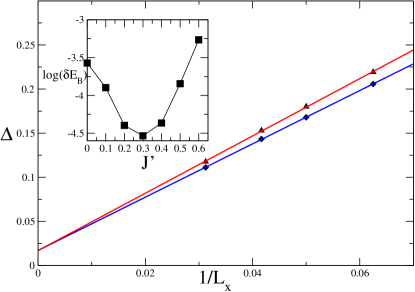
Figure 2: Finite size spin gap of 2D lattices (triangles) versus that of a single chain (diamonds). In the inset, error in the binding energy $\delta E_{B}=|E_{B}-E_{B}^{ED}|$ (in log scale) as a function of $J"$ for $J^{\prime}=0.3$.

We now concentrate on to the regime $J"=J^{\prime}$. The possibility of a disordered critical state was raised by the series expansion study of Refseries . The expansion becomes inacurate for small values of $J^{\prime}/J$, these authors could not reach this critical regime. Our data show the existence of such a disordered state for $J^{\prime}=J"=0.15$, $0.3$, and $0.45$. Fig. 2 shows for $J"=J^{\prime}=0.3$ the finite size gap $\Delta_{2D}$ of the 2D system and that of a single chain $\Delta_{1D}$. $\Delta_{2D}$ is found to be always smaller than $\Delta_{1D}$. Since $\Delta_{1D}\rightarrow 0$ when $L\rightarrow\infty$ and $m\rightarrow\infty$, we can thus conclude that the 2D system is also gapless in the thermodynamic limit. The 1D version of this model, the two-leg zigzag ladder white-affleck , has an exponentially small gap ($\Delta_{1D}\propto\exp(-\alpha J"/J)$ and $\alpha$ is a constant) hard to extrapolate from a finite size analysis. That small gap coexists with ferromagnetic correlations between adjacent spins on the weakest bonds of the dimerized states. None of these concurrent signatures of the 1D frustrated system are observed in the 2D model where the ferromagnetic correlations favor a collinear state.

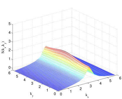
Figure 3: $S(k_{x},k_{y})$ for $L_{x}\times L_{y}=24\times 25$, $J^{\prime}=0.3$ and $J"=0.3$.

For $J^{\prime}=J"$, $S(k_{x},k_{y})$ shown in Fig. 3 is structureless in the $k_{y}$ direction and it retains its maximum at $\pi$ in the $k_{x}$ direction. This indicates that the chains are disconnected. The small bump which can be observed in $S(k_{x},k_{y})$ near $(\pi,\pi)$ is a consequence of very small short-range transverse AFM correlations. Thus the spin liquid state is mostly 1D. Our conclusion of a disconnected chains ground state is also supported by the transverse local bond strength $|\langle{\bf S}_{il}{\bf S}_{il+1}\rangle|$ and the binding energy of the chains $E_{B}=E_{1D}-E_{2D}/(L+1)$ (not shown), where $E_{1D}$ is the ground state energy of a chain of length $L$ and $E_{2D}$ the ground state energy of a $L\times L+1$ lattice. $|\langle{\bf S}_{il}{\bf S}_{il+1}\rangle|$ decays from $0.0818$ in the Néel state ($J^{\prime}=0.3$, $J"=0$) and $0.0766$ in the collinear state ($J^{\prime}=0.3$, $J"=0.6$) to $0.0132$ in the disordered state ($J^{\prime}=0.3$, $J"=0.3$).

Indeed, one expects the perturbative DMRG method to be valid only at small couplings. One may thus question its validity for relatively large couplings such as $J^{\prime}=J"=0.3$, and $0.45$. In Refalvarez-ED we have shown that, when larger values of the transverse coupling are used, the two-step DMRG is indeed less accurate when a genuine two-dimensional state emerges. But at the maximally frustrated point (which is at $J^{\prime}=J"$) the method remains surprisingly accurate even for intermediate values of $J^{\prime}$ and $J"$. This is seen in the inset of Fig.2 which shows that $\delta E_{B}$, the difference in binding energy between the perturbative DMRG and exact diagonalization, is minimum at $J^{\prime}=J"$. This is because at the maximally frustrated point, the interchain correlations are very small. Thus consistent with the observation made on $S(k_{x},k_{y})$, in the ground state, the eigenstates of an isolated chains are a good approximation for the 2D system.

We now study the stability of the 2D spin liquid state against interplane perturbations. The 3D results are less accurate than the 2D ones. The maximum truncation error was about $10^{-3}$ during the generations of the effective 2D Hamiltonian to be used as the starting point in the 3D computations. This relatively large truncation error is due to the fact that five spin sectors are targeted. We thus were restricted to smaller 2D lattices. The largest lattice we studied was $16\times 16\times 17$. We set $J^{\prime}=J"=0.3$ and we vary $J_{z}$ from $0.05$ to $0.15$. Fig. 4 displays $S(k_{x},k_{y})$ for $J_{z}=0.2$ in the middle plane, i.e. the $9^{th}$ plane in a $16\times 16\times 17$ lattice. One can observe the emergence of a small peak at $(\pi,\pi)$ which is due to the interplane coupling. We find that as one may expect, the height of this peak increases with increasing $J_{z}$. Since the coupling in the third direction is not frustrated, magnetic energy can be gained by coupling the planes. As a consequence, the spin liquid state which results from the inability of the chains within the planes to couple effectively is destroyed.

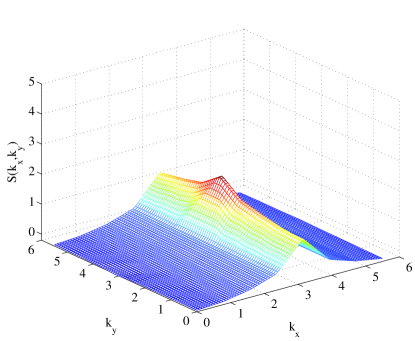
Figure 4: $S(k_{x},k_{y})$ for $L_{x}\times L_{y}=16\times 16$, $J^{\prime}=0.3$, $J"=0.3$ and $J_{z}=0.15$.

To summarize, we have studied the ground state properties of a 3D anisotropic Heisenberg model. We can now address the issues mentioned in the introduction which were motivated by the experimental results of Ref.coldea . (i) In the 2D regime of this model, the magnetic structure factor, the binding energy display the properties of a spin liquid state. This spin liquid state separate two regimes with long-range order. (ii) This spin liquid state is gapless and is made of nearly independent chains. It is remarkable that it survives even when the interchain exchange are of the same magnitude as the intrachain exchange. Since it has been previously reported in the crossed chain model singh and on a square lattice, it seems to be generic of models of chains coupled with a frustrating interaction. (iii) Turning on the interplane coupling restores magnetism. But we do not find any tendency to incommensurate ordering. The discrepancy on this point between our simulation and the experiment coldea may be due to the fact that in the compound Cs₂CuCl₄, consecutives triangular layers are sligthly rotated from each other. This effect can be taken into account by adding a Dzyaloshinskii-Moriya interaction into the Hamiltonian(1). This term could be the source of the incommensurate ordering.

- (1) M.F. Collins and O.A. Petrenko, Can. J. Phys. 75, 605 (1997).
- (2) R. Coldea et. al., Phys. Rev. Lett. 86, 1335 (2001); Phys. Rev. B 68, 134424 (2003).
- (3) Z. Weihong, Ross H. McKenzie, R. R. P. Singh Phys. Rev. B 59, 14367 (1999).
- (4) M. Bocquet, F.H.L. Essler, A. M. Tsvelik, A. O. Gogolin Phys. Rev. B 64, 094425 (2001).
- (5) S. Moukouri and L.G. Caron, Phys. Rev. B 67, 092405 (2003).
- (6) S. Moukouri cond-mat/0305608 (unpublished).
- (7) S. Moukouri physics/0312011 (to appear in Phys. Lett. A).
- (8) J.V. Alvarez and S. Moukouri cond-mat/0402530 (unpublished).
- (9) T. Kato, Prog. Teor. Phys. 4, 514 (1949); 5, 95 (1950).
- (10) C. Bloch, Nucl. Phys. 6, 329 (1958).
- (11) S.R. White, Phys. Rev. Lett. 69, 2863 (1992). Phys. Rev. B 48, 10 345 (1993).
- (12) E. Dagotto and A. Moreo, Phys. Rev. Lett. 63, 2148 (1989).
- (13) P. Chandra, P. Coleman and A.I. Larkin, Phys. Rev. Lett. 64, 88 (1990).
- (14) S.R. White and I. Affleck, Phys. Rev. B 54, 9862 (1996).
- (15) O.A. Starykh, R.R.P. Singh and G.C. Levine, Phys. Rev. Lett. 88, 167203 (2002).