Collective edge modes in fractional quantum Hall systems

Abstract

Over the past few years one of us (Murthy) in collaboration with R. Shankar has developed an extended Hamiltonian formalism capable of describing the ground state and low energy excitations in the fractional quantum Hall regime. The Hamiltonian, expressed in terms of Composite Fermion operators, incorporates all the nonperturbative features of the fractional Hall regime, so that conventional many-body approximations such as Hartree-Fock and time-dependent Hartree-Fock are applicable. We apply this formalism to develop a microscopic theory of the collective edge modes in fractional quantum Hall regime. We present the results for edge mode dispersions at principal filling factors $\nu=1/3,1/5$ and $\nu=2/5$ for systems with unreconstructed edges. The primary advantage of the method is that one works in the thermodynamic limit right from the beginning, thus avoiding the finite-size effects which ultimately limit exact diagonalization studies.

I Introduction

The bulk fractional quantum Hall effect is by now well-understood as a consequence of an interaction-driven incompressible statelaugh ; jain ; fqhereviews of a two-dimensional electron gas (2DEG) in a strong perpendicular magnetic field. It was also realized long agohalperin that the edges of the bulk system play a fundamental role in transport at low frequencies, since the bulk is incompressible and the gapless excitations are available only at the edges. An effective description of edge excitations for incompressible fractions was first proposed by Wen.wen He developed a hydrodynamic theory of a sharp edge, which is a realization of the one-dimensional Chiral Luttinger liquid.

Recently, several high-precision experiments have probed the low-frequency dynamics of the edge in the fractional quantum Hall (FQH) regime over a range of filling factors.expts ; lloyd Some features of the results, such as the observation of a power law in the $I$-$V$ curve which depends on the filling factor, and the magnitude of the power-law exponent,expts are unexpected from the point of view of hydrodynamic theories of the edge.wen ; kane Many explanations have been proposed for these discrepancies,dhlee ; ana ; ulrich ; levitov ; goldman ; wan ; mandal ; kun including the effects of long-range interactions and edge reconstructions. Motivated by these experiments, Wan et al.wan have recently explored the effects of edge reconstructions on the behavior of the collective modes using numerical exact diagonalization. While important qualitatively new resultskun have been obtained by this research, these studies do suffer from finite-size effects.

We want to investigate the physics of FQH edges using the extended Hamiltonian theory developed by Shankar and Murthy.sm1 This approach has the advantages that it starts with a microscopic Hamiltonian, permits analytic calculations in the thermodynamic limit and also retains the lowest Landau level limit. It thus provides a complementary approach to that of exact diagonalization studies. In a previous paperyogesh we applied the extended Hamiltonian theory to study the structure of FQH edges within the Hartree-Fock (HF) approximation. In this paper, we further explore the edge states beyond mean-field level. We use the time-dependent Hartree-Fock (TDHF) approximation which systematically incorporates particle-hole states because it is a conserving approximation,conserving i.e. it respects the symmetries of the problem.

The structure of our paper is as follows: In the next section, we review the essentials of the extended Hamiltonian theory and mean-field theory of FQH edges. The time-dependent Hartree-Fock approximation is described in Section III. Our numerical results for $\nu=1/3,1/5$ and $\nu=2/5$ are presented in Section IV. The results for $\nu=2/5$ are, to the best of our knowledge, the first in the literature. The last section contains conclusions and caveats. Throughout this paper we restrict ourselves to unreconstructed edges due to the computational limitations of our own.

II Extended Hamiltonian theory and Hartree-Fock approximation

For a two-dimensional electron gas in a strong perpendicular magnetic field, the kinetic energy of electrons is quenched and the single-particle states are organized into Landau levels separated by the cyclotron energy. For electrons in the lowest Landau level, neglecting the zero point energy, the interaction Hamiltonian is given by

$$H_{e}=\frac{1}{2A}\sum_{\vec{q}}V_{ee}(\vec{q}):\rho_{e}(\vec{q})\rho_{e}(-\vec{q}):$$ (1)

where $V_{ee}(\vec{q})$ is the repulsive electron-electron interaction. This interaction energy scale is typically several tens of Kelvins, of the same order as the cyclotron energy (about 100K). Nevertheless, in the integer quantum Hall regime, the interaction is usually treated as a perturbation on the ground-state Slater-determinant of $\nu$ Landau levels completely filled. For a fractional filling factor, this ground state is degenerate and the perturbative approach fails.laugh The key insight of Jainjain was that if one thinks in terms of Composite Fermions (CFs), which are envisioned as electrons attached to an even number $2s$ of flux quanta, one can use the independent particle picture for the Composite Fermions. In this approach, a system at filling factor $\nu=p/(2ps+1)$ has CFs which see an effective field $B^{*}=B/(2ps+1)$, which is just right for them to fill $p$ CF Landau levels (CF-LLs). Based on this insight, Jain constructed excellent wavefunctions for ground state and low-lying excited states for the principal filling factors. However in order to calculate response functions or finite-temperature properties, one needs a dynamical theory. Initial attempts focused on bosonicbosonic or fermionicfermionic variants of the Chern-Simons theorycs culminatingkalmeyer in a Chern-Simons theory for $\nu=1/2$, which is a Fermi-liquid-like state.nu-half These theories, while satisfactory in many respects, still did not incorporate some of the nonperturbative aspects of the CF, such as the facts that in the lowest-Landau-level limit the effective mass of the CF is determined by the interactions alone or that its charge is fractional.

To handle these problems, Shankar and Murthy developed the extended Hamiltonian theory,sm1 a detailed account of which can be found in a recent review.rmpus A key ingredient of this theory is the introduction of a new set of coordinates for pseudovortices in addition to those of electrons. For a FQH liquid at filling factor $\nu=p/(2ps+1)$ where $p$ and $s$ are integers, each electron couples with $2s$ pseudovortices to form a composite fermion (CF) in the following way

$$\vec{R_{e}} = \vec{r}-\frac{l^{2}}{1+c}\hat{z}\times\vec{\Pi},$$ (2)

$$\vec{R_{v}} = \vec{r}+\frac{l^{2}}{c(1+c)}\hat{z}\times\vec{\Pi},$$ (3)

where $c^{2}=2\nu s$, $l=\sqrt{h/eB}$ and $\vec{r}$ and $\vec{\Pi}$ are the position and velocity operators of the composite fermion. The electron guiding center $\vec{R_{e}}$ and the pseudovortex guiding center $\vec{R_{v}}$ satisfy the algebra

$$[R_{e\alpha},R_{v\beta}] = 0,$$ (4)

$$[R_{e\alpha},R_{e\beta}] = -il^{2}\epsilon_{\alpha\beta},$$

$$[R_{v\alpha},R_{v\beta}] = +i\frac{l^{2}}{c^{2}}\epsilon_{\alpha\beta}.$$

Thus, the electron guiding-center coordinates satisfy the magnetic algebra with charge $-e<0$, whereas the pseudovortex guiding-center algebra represents an object with charge $+ec^{2}$. The CFs thus have a magnetic algebra charge of $e^{*}=-e(1-c^{2})$, showing that they are subject to a reduced magnetic field $B^{*}=B/(2ps+1)$, just right to fill the first $p$ CF-Landau levels, exactly as in Jain’s picture.jain The Hartree-Fock state of CFs with the first $p$ Landau levels filled provides a nondegenerate starting point for analytical calculations.

To calculate the matrix elements of these operators in the CF basis, we use the single-particle states of the CFs in the reduced effective field $B^{*}$. In the Landau gauge, a single-particle state $|nX\rangle$ is characterized by the CF-Landau level index $n$ and the guiding-center coordinate $X$. In the real-space representation, the (unnormalized) single-particle wavefunction is

$$\langle\vec{r}|nX\rangle=e^{iXy/l^{*^{2}}}e^{-(x-X)^{2}/2l^{*^{2}}}H_{n}\left[(x-X)/l^{*}\right],$$ (5)

where $H_{n}(x)$ are the Hermite polynomials and $l^{*}=\sqrt{h/eB^{*}}$ is the magnetic length in the reduced field $B^{*}$ seen by the CFs. In the following, we use $l^{*}=1$ as the unit of length. Using this basis, it is straightforward to express the electron density $\rho_{e}$ and the pseudovortex density $\rho_{v}$ operators in second-quantized notation

$$\rho_{e}(\vec{q}) = \sum_{n_{i}X}e^{-iq_{x}X}d^{\dagger}_{n_{1}X-q_{y}/2}d_{n_{2}X+q_{y}/2}\rho_{n_{1}n_{2}}(\vec{q}),$$ (6)

$$\rho_{v}(\vec{q}) = \sum_{\nu X}e^{-iq_{x}X}d^{\dagger}_{n_{1}X-q_{y}/2}d_{n_{2}X+q_{y}/2}\chi_{n_{1}n_{2}}(\vec{q}),$$ (7)

where $d_{nX}(d^{\dagger}_{nX})$ destroys (creates) a CF in the state $|nX\rangle$, and $\rho_{n_{1}n_{2}}$ ($\chi_{n_{1}n_{2}}$) are the plane-wave matrix elements for electron guiding center $\vec{R}_{e}$ (pseudovortex guiding center $\vec{R}_{v}$).rmpus We have now expressed the electron density operators and hence the microscopic Hamiltonian for the fractional quantum Hall systems in terms of CF operators, $d_{nX}$ and $d^{\dagger}_{nX}$. Therefore the original problem of interacting electrons in the fractional quantum Hall regime has been readily transformed into a problem of CFs in the integer quantum Hall regime where various many-body approximations are applicable. But, we must remember that there is no free lunch; the price to pay is that the transformed problem is subject to special constraints as a result of the introduction of pseudovortex coordinates (section III).

We next consider the positive neutralizing background charge $\rho_{b}(x)$ which produces a confining potential near the edge at $x=0$. The corresponding Hamiltonian is

$$H_{b} = \sum_{\vec{q}}{V}_{eb}(-\vec{q})\rho_{e}(\vec{q})$$ (8)

where

$$V_{eb}(x)=\int^{\infty}_{-\infty}dx^{\prime}\,V_{eb}(x-x^{\prime})\rho_{b}(x^{\prime}),$$ (9)

and $V_{eb}(x)$ is the attractive electron-background interaction. We choose a background charge density which vanishes linearly over width $W$ near the edge: $\rho_{b}(x)=0$ for $x<-W/2$, $\rho_{b}(x)=-\frac{\rho_{0}}{2}\left[1+\frac{2x}{W}\right]$ for $|x|<W/2$, and $\rho_{b}(x)=\rho_{0}$ for $x>W/2$ where $\rho_{0}$ is the CF density in the bulk.chamon ; yogesh We also assume that the background charge resides in the same plane as the 2DEG, $V_{eb}(\vec{q})=-V_{ee}(\vec{q})$.

In the bulk of a FQH liquid at filling factor $\nu=p/(2ps+1)$, $p$ CF Landau levels are completely filled. Due to the presence of the confining potential close to the edge, different CF-LLs mix together. Since the system is still translationally invariant along the $y$-direction, the Landau gauge quantum number $X$ is a good quantum number, and only CF-LLs with the same value of $X$ mix. We introduce the mixing matrices $\alpha(X)$ as function of $X$

$$d_{nX}=\sum_{m}\alpha_{nm}(X)a_{mX}$$ (10)

where $a_{mX}$ denote the annihilation operators for the CF quasiparticles which result from mixing of different CF-LLs. The total Hamiltonian, $H_{e}+H_{b}$, represented in terms of new operators $a_{mX}$ and $a^{\dagger}_{mX}$, is decoupled using standard HF approximation rmpus and the mean-field solution is chosen to be

$$\langle a^{\dagger}_{mX}a_{nX^{\prime}}\rangle=\delta_{mn}\delta_{XX^{\prime}}N^{F}_{m}(X)$$ (11)

where $N^{F}_{m}(X)$ is the CF-occupation number at guiding center $X$ and CF Landau level $m$. Note that with this ansatz for the mean-field solution we are explicitly forbidding any structure in the $y$-direction. Upon decoupling, the mean-field Hamiltonian becomes

$$H^{HF} = \sum_{mnX}H_{mn}(X)a^{\dagger}_{mX}a_{nX}$$ (12)

We determine the mixing matrices $\alpha$’s so that the mean-field Hamiltonian $H^{HF}$ is diagonal. The process is normally carried out iteratively as in our previous work. yogesh The quantities of interest in mean-field study are the energy bands $E_{m}(X)=H_{mm}(X)$, the occupation functions $N^{F}_{m}(X)$, and the mixing matrices $\alpha(X)$.

III Time-dependent Hartree-Fock Approximation

III.1 Time-dependent Hartree-Fock Hamiltonian

As we mentioned earlier, special care is required in treating the transformed Hamiltonian. In particular, the original electronic Hamiltonian knows nothing about the pseudovortex density $\rho_{v}$ and thus is invariant with respect to our choice of it. The transformed problem has extra degrees of freedom, the pseudovortex coordinates. Exact solutions to this problem will automatically be degenerate along the pseudovortex manifold, and will thus have a gauge symmetry. However, the mean-field ground state does not have the required gauge invariance. The situation is similar in the theory of superconductivity, where the Bardeen-Cooper-Schrieffer (BCS) ground state is not gauge invariant. Nonetheless gauge-invariant dynamical response functions can still be obtained from the mean-field ground state by a so-called conserving approximation.conserving TDHF approximation turns out to be the simplest of the class of conserving approximations, and is standard in the context of superconductivity when dealing with the gauge symmetry.conserving Read was the first to apply the TDHF approximation to study the problem of $\nu=1$ bosons,nu1bosons which has important similarities to the FQH system at filling factor $\nu=1/2$.nu-half It was subsequently used by MurthyGanpathy to find the collective modes for the incompressible fractions using the extended Hamiltonian theory.

In this Section, we will exploit the TDHF approximation to obtain the dispersion relations of the edge excitations. The way the conserving nature of the TDHF approximation manifests itself is that the spectrum of the TDHF Hamiltonian necessarily contains zero eigenvalues, each corresponding to an unphysical gauge degree of freedom, while the rest of the spectrum is physical. Ganpathy It is important that the unphysical zero-modes are identified and excluded and we will discuss the techniques we use for the same in the next subsection.

It follows from Eq.(4) that $\left[\rho_{e}(\vec{q}),\rho_{v}({\vec{q}}^{\prime})\right]=0.$ The total Hamiltonian, $H_{e}+H_{b}$, therefore commutes with the pseudovortex density $\rho_{v}$. Let us consider the magnetoexciton operator

$$O_{m_{1}m_{2}}(X,q_{y})=a^{\dagger}_{m_{1},X-q_{y}/2}a_{m_{2},X+q_{y}/2}$$ (13)

where $a_{mX}$ is the rotated annihilation operator related to the CF-operator $d$ as in Eq. (10). We have explicitly made use of the fact that there is translational invariance in the $y$-direction and therefore $q_{y}$ is a good quantum number. Henceforth we shall suppress the index $q_{y}$ and simply write $O_{m_{1}m_{2}}(X)$. The equation of motion for the magnetoexciton operator is

$$-i\frac{\partial}{\partial t}O_{m_{1}m_{2}}(X)=[H,O_{m_{1}m_{2}}(X)]$$ (14)

Using the standard HF decoupling to evaluate the right-hand-side we get

$$\left[H,O_{m_{1}m_{2}}(X_{0})\right] \rightarrow [E_{m_{1}}(X_{0}-q_{y}/2)-E_{m_{2}}(X_{0}+q_{y}/2)]O_{m_{1}m_{2}}(X_{0})+[N^{F}_{m_{1},X_{0}-q_{y}/2}-N^{F}_{m_{2},X_{0}+q_{y}/2}]$$ (15)

$$\times\sum_{X\nu k_{i}k^{\prime}_{i}}\left[h_{k_{1}k_{2}^{\prime}k_{1}^{\prime}k_{2}}(X_{0}-X,-q_{y})-h_{k_{1}k_{2}k_{1}^{\prime}k_{2}^{\prime}}(X-X_{0},q_{y})\right]$$

$$\times\ \ \alpha^{\dagger}_{k_{1}n_{1}}(X-q_{y}/2)\alpha_{k_{2}n_{2}}(X+q_{y}/2)\alpha^{\dagger}_{k_{1}^{\prime}m_{2}}(X_{0}+q_{y}/2)\alpha_{k_{2}^{\prime}m_{1}}(X_{0}-q_{y}/2)O_{n_{1}n_{2}}(X)$$

where

$$h_{k_{1}k_{2}k_{1}^{\prime}k_{2}^{\prime}}(X,q_{y})=\int\frac{dq_{x}}{2\pi}V_{ee}(\vec{q})\rho_{k_{1}k_{2}}(\vec{q})\rho_{k_{1}^{\prime}k_{2}^{\prime}}(-\vec{q})e^{-iq_{x}X}$$ (16)

and $\mu=(m_{1},m_{2})$, $\nu=(n_{1},n_{2})$ etc. We define a vector $\Psi_{\mu}(X)$ corresponding to the operator

$$O_{\Psi}=\sum_{\mu X}\Psi_{\mu}(X)O_{\mu}(X).$$ (17)

In the space spanned by $O_{\Psi}$, the TDHF Hamiltonian reads

$${\cal H}(\mu,\nu;X_{0},X;q_{y}) = \delta_{m_{1}n_{1}}\delta_{m_{2}n_{2}}[E_{m_{1}}(X_{0}-q_{y}/2)-E_{m_{2}}(X_{0}+q_{y}/2)]+[N^{F}_{m_{1},X_{0}-q_{y}/2}-N^{F}_{m_{2},X_{0}+q_{y}/2}]$$ (18)

$$\times\sum_{k_{i},k^{\prime}_{i}}\left[h_{k_{1}k_{2}^{\prime}k_{1}^{\prime}k_{2}}(X_{0}-X,-q_{y})-h_{k_{1}k_{2}k_{1}^{\prime}k_{2}^{\prime}}(X-X_{0},q_{y})\right]$$

$$\times\ \ \alpha^{\dagger}_{k_{1}n_{1}}(X-q_{y}/2)\alpha_{k_{2}n_{2}}(X+q_{y}/2)\alpha^{\dagger}_{k_{1}^{\prime}m_{2}}(X_{0}+q_{y}/2)\alpha_{k_{2}^{\prime}m_{1}}(X_{0}-q_{y}/2)$$

The TDHF Hamiltonian is the key quantity containing information about the collective modes in the system. Upon diagonalization, we obtain the energy spectrum of excitations, and the left ($\psi^{L}$) and right ($\psi^{R}$) eigenvectors. Direct inspection of Eqs.(16) and (18) shows that $\cal H$ changes sign, after a suitable reshuffling of indices, as $q_{y}$ does. That means the spectrum at a $q_{y}$ contains information about the spectrum at $-q_{y}$ as well. The left- and right-eigenvectors are identical (modulo reshuffled indices) for both $\pm q_{y}$. We are interested in the gapless excitations across the edge. These modes are in the regime of low energy and momentum, and our task at hand is to identify these modes from the energy spectrum.

III.2 Identification of the Physical Modes

Due to the gauge symmetry of the original Hamiltonian the TDHF Hamiltonian $\cal H$ necessarily has zero eigenvalues, even for a nonuniform system. In the exact solution of the original Hamiltonian each energy level is infinitely degenerate since it costs no energy to rotate among gauge-connected eigenstates. The zero modes of $\cal H$ are thus unphysical and we have to discard them from its spectrum. We stress that the spurious modes have precisely zero energy only when the full set of infinite CF-LLs are taken into account. Obviously, in computations, though one tries to include as many CF-LLs as possible, that number cannot be infinite. Therefore, the technical problem of how to separate the unphysical modes from the low-lying physical ones arises. There are two different ways to achieve this. The first one is to monitor the behavior of the energy of a mode. As more CF-LLs are added, the energy of an unphysical mode gets closer to zero while that of a physical mode becomes stable. In the bulk case the unphysical modes were singled out successfully using this procedure.Ganpathy The second is to resort to the electron density correlation function. Since the electron density operator is gauge-invariant, unphysical modes should decouple from its correlation functions as more CF-LLs are added.

In the edge case, the first method is not practical because the energy spectrum of $\cal H$ contains every mode at a given $q_{y}$ including many unphysical modes which have high $q_{x}$ and therefore require a very large number of CF-LLs for their detection. We shall instead use the second method. We define the electron density correlation function

$$S(X_{0},X^{\prime}_{0};q_{y},\omega)=-i\langle\rho_{e}(X_{0},q_{y},\omega)\rho_{e}(X_{0}^{\prime},-q_{y},-\omega)\rangle$$ (19)

as the ground-state expectation of a four-fermion operator. A detailed but straightforward calculation gives rise to the following expression for the density correlator in terms of known quantities,

$$S(X_{0},X^{\prime}_{0};q_{y},\omega) = \frac{A}{2\pi}\sum_{\alpha,k_{i}}\left[\sum_{\mu X}\rho_{m_{1}m_{2}}(X_{0}-X,q_{y})\psi^{R(\alpha)}_{k_{1}k_{2}}(X,q_{y})\alpha^{\dagger}_{m_{1}k_{1}}(X-q_{y}/2)\alpha_{m_{2}k_{2}}(X+q_{y}/2)\right]$$ (20)

$$\times\left[\sum_{\nu X^{\prime}}\rho_{n_{1}n_{2}}(X^{\prime}_{0}-X^{\prime},-q_{y})\psi^{L(\alpha)}_{k_{4}k_{3}}(X^{\prime},-q_{y})\alpha^{\dagger}_{n_{1}k_{3}}(X^{\prime}+q_{y}/2)\alpha_{n_{2}k_{4}}(X^{\prime}-q_{y}/2)\right]$$

$$\times\left[N^{F}_{k_{3}}(X^{\prime}+q_{y}/2)-N^{F}_{k_{4}}(X^{\prime}-q_{y}/2)\right]\left(\omega-E_{\alpha}+i\eta\,sign(E_{\alpha})\right)^{-1}$$

where $\rho_{\mu}(X,q_{y})$ is the 1D Fourier transform of the density matrix

$$\rho_{\mu}(X,q_{y})=\int\frac{dq_{x}}{2\pi}\,e^{iq_{x}X}\rho_{\mu}(q_{x},q_{y})$$ (21)

As handy as it looks, Eq. (20) still has a minor technical problem. It describes how strongly a mode couples with the electron density; in other words, while it does discriminate between physical and unphysical modes, it does not discriminate between the bulk and edge modes. We note that physical edge modes at low momentum and energy, the regime of interest, should become stable as more and more CF-LLs are added. In a further refinement we exclude the high-momentum modes by the following filtering procedure. Let us consider, instead of the pure electron density $\rho_{e}$ used in Eq.(20), a filtered operator concentrated near the edge

$$\rho^{f}_{\mu}(X_{0},q_{y})=\sum_{X}e^{-(X-X_{0})^{2}/2l^{2}_{f}}\ \rho_{\mu}(X,q_{y})$$ (22)

that cuts off all fluctuations across the edge with length-scales longer than $l_{f}$. The choice of Gaussian filtering in Eq.(22) is convenient for calculations. The results we present in the following section are based on the choice $l_{f}=l^{*}$, which seems to work well. The filtered density correlator, $S^{f}(X_{0},X^{\prime}_{0};q_{y},\omega)=-i\langle\rho^{f}_{e}(X_{0},q_{y},\omega)\rho^{f}_{e}(X^{\prime}_{0},-q_{y},-\omega)\rangle$ satisfies exactly the same formula (20) except that the electronic density matrix elements $\rho_{\mu}(X,q_{y})$ are replaced by the filtered density ones $\rho^{f}_{\mu}(X,q_{y})$, defined as

$$\rho^{f}_{\mu}(X,q_{y})=\int\frac{dq_{x}}{2\pi}\,e^{-q_{x}^{2}l_{f}^{2}/2+iq_{x}X}\rho_{\mu}(q_{x},q_{y})$$ (23)

IV Results

In the following calculations, we vary the confining potential at the edge by changing the width $W$ over which the background charge vanishes linearly from its bulk value to zero. We consider a short-ranged Gaussian interaction

$$V_{ee}(\vec{q})=V_{0}e^{-q^{2}\,\lambda^{2}/2}=-V_{eb}(\vec{q})$$ (24)

with range $\lambda=l^{*}$, and a Thomas-Fermi interaction

$$V_{ee}\vec{q})=\frac{2\pi e^{2}}{\sqrt{q^{2}+q_{TF}^{2}}}=-V_{eb}(\vec{q})$$ (25)

with $q_{TF}l^{*}=0.4$, which becomes truly long ranged as $q_{TF}\rightarrow 0$. The Thomas-Fermi case is considerably more difficult for the HF part of the calculation. As $q_{TF}$ decreases, it takes more iterations for the HF to converge and the presence of the edge makes itself felt deeper inside the bulk. We do not find any qualitative difference in the edge collective modes between the two cases. This being the case, we concentrate on the short-range Gaussian interactions for $\nu=1/5$ and $\nu=2/5$.

Deep in the bulk, the quantum Hall liquid is uniform and the structure of CF-LLs and excitations in TDHF is well-understood. Ganpathy For numerical purposes we focus on the region around the edge, taking $8l^{*}$ in the bulk side and $2l^{*}$ in the empty side. The lattice spacing is $\Delta x=0.1l^{*}$, resulting in 100 sites. Typically, 8 to 10 CF-LLs are considered. The TDHF Hamiltonian size is of the order of a few thousand, making the diagonalization feasible. Notice that $\Delta x$ sets the lower bound on resolution for $q_{y}$ (recall that the magnetoexciton contains CF creation and destruction operators separated by distance $q_{y}$.) We believe that our choice of $\Delta x=0.1l^{*}$ is appropriate as the natural length-scale in the problem is $l^{*}$. Reducing $\Delta x$, while allowing us to explore smaller values of $q_{y}$, would require more computational resources.

Figure 1: Typical mean-field energy bands (left) and electron density profile (right) at the edge for $\nu=1/3$. We have used the Gaussian interaction, $W=0$ and 10 CF-LLs. The energy is measured in units of $e^{2}/\epsilon l^{*}$ and length is measured in units of $l^{*}$ (Note that our interaction is not normalized). Only one CF-LL is occupied in the bulk, as signified by the bulk electron density $\rho_{e}=1$ in the right panel; the dotted line in the left panel denotes the chemical potential.

First we present results for the $\nu=1/3$ case, which corresponds to $s=1=p$ or $c=\sqrt{2/3}$. In this case, the ground state in the bulk has only the lowest CF-LL filled. We solve the HF mean-field equations to obtain the energy bands, the mixing matrices, and the CF occupation profile. Figure 1 shows typical mean-field energy bands (left) and electron density profile (right) near the edge for a Gaussian interaction, with $W=0$ and 10 CF-LLs. From the mean-field results the TDHF Hamiltonian $\cal H$, Eq.(18), is created and diagonalized. A direct inspection of $\cal H$ reveals that only the excitations from the lowest CF-LL to higher ones are relevant to the edge modes. We thus need to keep only elements in $\cal H$ that have $m_{1}=0$ or $m_{2}=0$. The size of the TDHF Hamiltonian with 10 CF-LLs is $100\times 19=1,900$ rows (and columns). While diagonalizing a matrix this size is easy, the most time-consuming part of the computation is the evaluation of the matrix $\cal H$ due to the quadruple sum in Eq. (18). Although the TDHF Hamiltonian is not symmetric, remarkably, our diagonalization results find that it only possesses real eigenvalues, meaning every mode is long-lived as normally expected. Upon diagonalization, the set of left- and right- eigenvectors are used to compute the filtered density correlator.

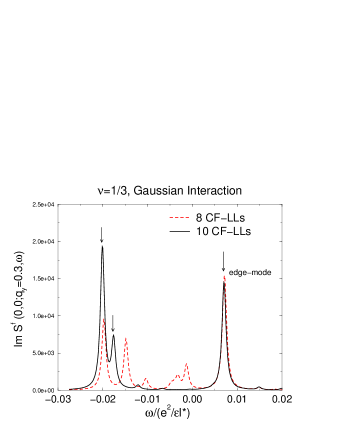
Figure 2: Spectral function of the local electron density correlator, Im $S^{f}(0,0;q_{y}=0.3,\omega)$ for a $\nu=1/3$ system with Gaussian interaction and $W=0$. The dotted (solid) lines show results with 8 (10) CF-LLs. The arrows indicate poles of physical edge modes. Notice that the spurious modes lying between the arrows are strongly suppressed as the number of CF-LLs is increased from 8 to 10, whereas the physical edge mode with positive energy remains essentially unchanged in both position and weight.

Figure 2 shows the imaginary part of the local filtered correlator $S^{f}(0,0;q_{y}=0.3,\omega)$. It is evident from the picture that while there are several peaks in Im $S^{f}$ at 8 CF-LLs, many of them at low energy disappear at 10 CF-LLs. These peaks represent spurious modes which decouple from the electron density in the limit of infinite number of CF-LLs. The arrows indicate peaks corresponding to the physical modes which are stable as more CF-LLs are added. The peak at positive energy is the edge mode; it changes little in position and weight as the number of CF-LLs is increased. The gradual disappearance of unphysical modes and the stability of the physical modes with respect to increasing number of CF-LLs are strong indications that our results, although obtained using a finite number of CF-LLs, are reliable.

Figure 3: Dispersion (left) and inverse velocity (right) of $\nu=1/3$ edge mode for a system with Gaussian interaction, $W=0$, and 10 CF-LLs. In the left panel, the dotted line is the naive mean-field result whereas the solid line is the dispersion obtained from TDHF approximation. The right panel shows the momentum-dependent inverse velocity $1/v(q)$ which fits the heuristic form (26). The suppression of velocity at large $q$ is due to the decreasing electron density near the edge.

By carrying out this procedure for different values of $q_{y}$ we obtain the dispersion relation for the $\nu=1/3$ edge mode, which is shown in Fig. 3. The TDHF approximation, which takes into account the collective particle-hole pair states, reduces the excitation energy below its mean-field value and is shown with a dotted line. As expected, the edge mode is gapless, and at small momenta the dispersion is linear, $\omega_{c}(q)=v_{0}q_{y}$, where $v_{0}$ is the cyclotron velocity of the CF along the edge. For larger momenta, we assume a momentum-dependent velocity $v(q)$. To see heuristically what the natural form of this velocity might be, note that as $q_{y}$ increases we are making excitations deeper into the empty region. In this region the electron density is smaller than that in the bulk and thus the effective field $B^{*}$ seen by the CFs must be larger. This means the velocity of excitations must be smaller. Assuming a linear variation of the electron density and thus the effective field near the edge (Fig. 1) we arrive at the following form,

$$\frac{1}{v(q)}=\frac{1}{v_{0}}+aq_{y}$$ (26)

where $v_{0}=v(q=0)$ and $a$ is a constant. The right panel in Fig. 3 shows the inverse CF velocity corresponding to the dispersion shown in the left panel. Given that there is only one free parameter $a$, the data seem to fit our ansatz (26) very well.

Now we examine how the collective mode dispersion changes as the width of the confining potential $W$ is increased. We remind the reader that as $W$ increases, the $\nu=1/3$ edge becomes susceptible to reconstruction irrespective of the range of electron-electron interaction.chamon ; yogesh Therefore we expect a substantial softening of the collective mode dispersion as a precursor to the edge reconstruction. Figure 4 shows the dispersion (left) and the inverse CF velocity (right) for $W=1.2l^{*}$; indeed, as expected, the dispersion for $W=1.2l^{*}$ is softer than that for $W=0$ (Fig. 3).

Figure 4: Dispersion (left) and inverse CF velocity (right) of the $\nu=1/3$ edge mode with Gaussian interaction, 10 CF-LLs and $W=1.2l^{*}$. Note that the edge mode softens as $W$ increases (Fig. 3).

To illustrate the effect of the range of interaction on the edge modes, we also study the $\nu=1/3$ case with Thomas-Fermi interaction. In this case, it is harder to filter out the spurious modes than in the case with short-ranged Gaussian interactions; however, our scheme still works reasonably well. Figure 5 shows the edge-mode dispersion (left) and inverse CF velocity (right) with $W=0$ and 10 CF-LLs. These results are qualitatively similar to those obtained using Gaussian interaction. The overall change in the edge-mode energy-scale is due to our use of un-normalized Gaussian interaction and has no fundamental significance.

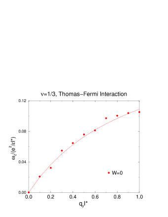
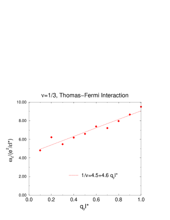
Figure 5: Dispersion (left) and inverse CF velocity (right) for $\nu=1/3$ state with Thomas-Fermi interaction, $W=0$, and 10 CF-LLs. Note that the dispersion is similar to that in the case of Gaussian interactions and our ansatz (26) for inverse velocity works for long-ranged interactions as well.

Next we consider filling factor $\nu=1/5$ which corresponds to CFs (consisting of electrons with $2s=4$ flux quanta) filling the lowest CF Landau level ($p=1$ and $c=\sqrt{4/5}$). Since there is no qualitative difference between collective edge modes obtained from Gaussian or Thomas-Fermi interactions, we concentrate on the Gaussian interaction which is more amenable to analytical calculations. Figure 6 shows the dispersion of the edge mode (left) and the inverse CF velocity (right), with $W=0$ and 10 CF-LLs. We note that the edge-mode energy scale is similar to that observed in the $\nu=1/3$ case. As expected, we find one edge mode and that mode softens with increasing $W$. We also find that the inverse CF velocity fits our heuristic form (26) and the free parameter $a$ has value similar to that in the $\nu=1/3$ case.

Figure 6: Dispersion (left) and inverse CF velocity (right) for the $\nu=1/5$ edge collective mode with Gaussian interaction, $W=0$ and 10 CF-LLs. The fit of the inverse CF velocity (right) to our heuristic form is still reasonable. The large scatter at small momenta arises from uncertainties in locating the physical edge mode at small energies.

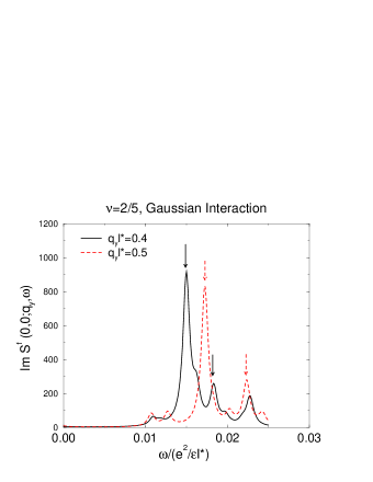
Figure 7: Spectral function of the local electron density correlator for $\nu=2/5$ with Gaussian interaction, $W=0$ and 8 CF-LLs. The positions of the physical edge modes, defined by their stability with increasing CF-LLs and their positive energies, are marked with arrows for $q_{y}l^{*}=0.4$ (solid) and $q_{y}l^{*}=0.5$ (dotted).

Let us now turn to the case of a fully spin-polarized $\nu=2/5$ state. Here we present, to the best of our knowledge, the first microscopic treatment of collective edge modes for $\nu=2/5$. In this case, the CFs (consisting of electrons with $2s=2$ flux quanta) fill $p=2$ CF Landau levels in the bulk, which leads to more involved numerical calculations. One now needs a TDHF matrix with twice the dimension as in the case of $\nu=1/3$ or $\nu=1/5$, since there are two filled CF-LLs in which the hole can be created. Consequently, we expect two gapless modes at the edge propagating in the same direction. Due to computational constraints, we restrict ourselves to Gaussian interaction and 8 CF-LLs. Figure 7 shows the spectral function of the local density correlator, Im $S^{f}(0,0;q_{y},\omega)$ for $q_{y}l^{*}=0.4$ and $q_{y}l^{*}=0.5$. For each value of $q_{y}$, two peaks marked by arrows represent the physical edge modes. It is interesting to note that contrary to the naive speculation, the edge mode with smaller energy has a greater spectral weight and therefore higher charge. Right panel in Fig. 8 shows dispersions for both edge modes, which have approximately the same velocity; the left panel shows that the inverse CF velocities can be fit to the heuristic form obtained earlier.

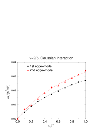
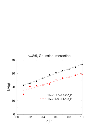
Figure 8: Dispersions (left) and inverse CF velocities of edge modes for a $\nu=2/5$ system with Gaussian interaction, $W=0$ and 8 CF-LLs. The two modes have similar velocities and their inverse CF velocities fit the ansatz (26) reasonably well.

V Discussion

In this paper we have presented a microscopic approach to calculating collective edge excitations in the fractional quantum Hall regime which is complementary to the exact diagonalization approach. This approach is based on the extended Hamiltonian theory rmpus and permits the use of many-body approximations which are generally valid in the integer quantum Hall regime. We have presented results for collective modes, and their dependence on the nature of electron-electron interaction and the width of the background confining potential at various filling factors. For an unreconstructed edge, at filling factor $\nu=1/3$ and $\nu=1/5$, we found a single linearly dispersing edge mode which softens with the increasing width $W$ of the confining potential. In contrast, we found two linearly dispersing modes for fully spin-polarized $\nu=2/5$ state. It is somewhat surprising that the two edge modes have nearly the same energy, and that the mode with the lower energy has a greater overlap with the charge operator. The curvature of the collective mode dispersion is somewhat unexpected from hydrodynamic theories. We show that it can be understood satisfactorily by assuming a momentum-dependent collective mode velocity, Eq.(26), which reflects the effect of decreasing electron density and the subsequent increase in the effective field $B^{*}$ seen by the CFs. Our ansatz implies that the magnetoexciton frequency $\omega_{c}(q)=v(q)q_{y}$ depends only on the combination $v_{0}q_{y}$. Incidentally, we find that the free parameter $a$ is roughly equal for $\nu=1/3$ dispersion and both branches of $\nu=2/5$ dispersion; therefore we can collapse all three dispersions (which have $s=1$) onto a single curve by scaling with $v_{0}$ (Fig. 9). Our results for edge-mode dispersions did not show the roton minimum near $q_{y}l^{*}\sim 1$ seen in exact diagonalization studies,wan presumably because the system is not close to edge reconstruction. yogesh

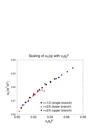
Figure 9: Scaling of the single-branch of $\nu=1/3$ dispersion and both branches of the $\nu=2/5$ dispersion with $v_{0}$. Since both have $s=1$, and similar values of the free parameter $a$ which appears in Eq.(26), the data collapse on a single curve.

Now let us mention some caveats. While our approach does not suffer from the computational limitations of exact diagonalization, we have computational limitations of our own. We work, in principle, in the thermodynamic limit. In practice, we are forced to truncate the filled states in the bulk and the empty states near the edge, to use a discretized Landau gauge index $X$, and to use a finite number of CF-LLs in the calculation. There are two limitations which we face: At the mean-field stage, we need to find the HF ground state as accurately as possible. Each step of the iterative HF calculation takes longer when these numbers get larger. In the TDHF stage, the main limitation is imposed by the time required to construct the TDHF matrix which involves a quadruple sum and increases as $N^{4}$ where $N$ is a measure of the number of single-particle levels kept. The diagonalization of the TDHF Hamiltonian takes a small fraction of the total computation time. We originally intended to study the softening of the collective edge-modes prior to edge reconstruction, and the evolution of edge-modes thereafter, as well. However, we were not successful in identifying the physical modes unambiguously at larger values of $W$. Presumably, with better computational resources, if we increase the number of CF-LLs used, this task will be feasible.

What our approach does is to bring within computational reach the techniques which have been successful in the study of edge modes of integer quantum Hall systems.chamon ; iqh-edge It does have its limitations; despite these limitations, we believe it can be usefully employed for cases which cannot be studied microscopically by any other method. For example, if one wants to calculate the temperature dependence of edge mode dispersion, one requires the knowledge of all excited states in an exact diagonalization approach. This is computationally prohibitive compared to finding the ground state and a few excited states. The state of the art exact diagonalization studies can treat at most 7-9 particles if all the states are kept.wan We expect the collective edge modes to be quite sensitive to temperature and finite size effects, since they are gapless. This may be the reason that although exact diagonalization studies with all stateswan reproduce the qualitative features of microwave absorption experiments,lloyd the energy scales predicted are considerably higher than those in the experiments. Another important piece of physics, which our approach can easily handle, is the role of disorder. In any real sample there is bound to be disorder. If the dominant disorder is due to quenched fluctuations in the remote dopant layer, the system breaks up into incompressible strips separated by compressible regions.efros These strips have been seen in imaging experiments.imaging It is straightforward to include the disorder potential perturbatively in our formulation, both in the mean-field and the TDHF approximations. The HF matrix is somewhat more complicated due to possible spatial structure along the edge. However, using the clean single-particle and collective modes of the incompressible strip as a basis, one can construct a microscopic theory of collective edge modes with disorder. This will provide us with a microscopic approach for examining the parameters which enter hydrodynamic theories to this problem.kane

One can also address novel edge-states with our approach, such as an edge between $\nu=1/3$ and $\nu=2/5$ regions which have CFs with the same number of flux quanta or an edge between $\nu=1/3$ and $\nu=2/9$ regions, which have CFs with different numbers of flux quanta attached. It would also be very interesting to study the edge dynamics of the Fermi-liquid-like state at $\nu=1/2$.eric

References

- (1) R.B. Laughlin, Phys. Rev. Lett. 50, 1395, (1983).
- (2) J.K. Jain, Phys. Rev. Lett. 63, 199 (1989); Phys. Rev. B 41, 7653 (1990); Science 266, 1199 (1994).
- (3) See, for example, Perspectives in Quantum Hall Effects, edited by S. Das Sarma and Aron Pinczuk (Wiley, New York, 1997); Composite Fermions, edited by Olle Heinonen (World Scientific, 1998).
- (4) B.I. Halperin, Phys. Rev. B 25, 2185 (1982).
- (5) X.G. Wen, Phys. Rev. Lett. 64, 2206 (1990); Phys. Rev. B 41, 12838 (1990); Int. J. Mod. Phys. B 6, 1711 (1992).
- (6) M. Grayson, D.C. Tsui, L.N. Pfeiffer, K.W. West, and A.M. Chang, Phys. Rev. Lett. 80, 1062 (1998); A.M. Chang, M.K. Wu, C.C. Chi, L.N. Pfeiffer, and K.W. West, Phys. Rev. Lett. 86, 143 (2001).
- (7) P.D. Ye, L.W. Engel, D.C. Tsui, J.A. Simmons, J.R. Wendt, G.A. Vawter, and J.L. Reno, Phys. Rev. B 65, 121305 (2002).
- (8) C.L. Kane and M.P.A. Fisher, Phys. Rev. Lett. 68, 1220 (1992); Phys. Rev. B 46, 15233 (1992); Phys. Rev. B 51, 13449 (1995).
- (9) D.H. Lee and X.G. Wen, cond-mat/9809160.
- (10) A. Lopez and E. Fradkin, Phys. Rev. B 59, 15323 (1999).
- (11) U. Zülicke and A.H. MacDonald, Phys. Rev. B 60, 1837 (1999).
- (12) L.S. Levitov, A.V. Shytov, and B.I. Halperin, Phys. Rev. B 64, 075322 (2001).
- (13) V.J. Goldman and E.V. Tsiper, Phys. Rev. Lett. 86, 5841 (2001).
- (14) X. Wan, K. Yang, and E.H. Rezayi, Phys. Rev. Lett. 88, 056802 (2001); X. Wan, E.H. Rezayi, and K. Yang, Phys. Rev. B 68, 125307 (2003).
- (15) S.S. Mandal and J.K. Jain, Phys. Rev. Lett. 89 096801 (2002).
- (16) K. Yang, Phys. Rev. Lett. 91, 036802 (2003).
- (17) R. Shankar and G. Murthy, Phys. Rev. Lett. 79, 4437 (1997).
- (18) Y.N. Joglekar, H.K. Nguyen, and G. Murthy, Phys. Rev. B 68, 035332 (2003).
- (19) G .Baym and L.P. Kadanoff, Phys. Rev. 124, 287 (1961); L.P. Kadanoff and G. Baym, Quantum Statistical Mechanics, (Addison-Wesley, Reading, MA, 1989).
- (20) S.M. Girvin and A.H. MacDonald, Phys. Rev. Lett. 58, 1252 (1987); S.C. Zhang, H. Hansson, and S.A. Kivelson, ibid. 62, 82 (1989); N. Read, ibid. 62, 86 (1989); D.H. Lee and S.C. Zhang, ibid. 66, 1220 (1991).
- (21) A. Lopez and E. Fradkin, Phys. Rev. Lett. 69, 2126 (1992).
- (22) J.M. Leinnas and J. Myrheim, Nuovo Cimento Soc. Ital. Fis., B 37, 1 (1977).
- (23) V. Kalmeyer and S.C. Zhang, Phys. Rev. B 46, 9889, (1992).
- (24) B.I. Halperin, P.A. Lee and N. Read, Phys. Rev. B 47, 7312, (1993).
- (25) G. Murthy and R. Shankar, Rev. Mod. Phys. 75, 1101 (2003).
- (26) C.de C. Chamon and X.G. Wen, Phys. Rev. B 49, 8227 (1994).
- (27) V. Pasquier and F.D.M. Haldane, Nucl. Phys. B 516, 719 (1998); N. Read, Phys. Rev. B 58, 16262 (1998).
- (28) G. Murthy, Phys. Rev. B, 64, 195310 (2001).
- (29) D.B. Chlovskii, B.I. Shklovskii, and L.I. Glatzman, Phys. Rev. B 46, 4026 (1992); A.H. MacDonald, S.R. Eric Yang, and M.D. Johnson, Aust. J. Phys. 46, 345 (1993); L. Brey, Phys. Rev. B 50, 11861 (1994); D.B. Chlovskii, Phys. Rev. B 51, 9895 (1995).
- (30) A.L. Efros, Solid State Commun. 65, 1281 (1988); ibid. 70, 253 (1989); Phys. Rev. B 45, 11354 (1992); A.L. Efros, F.G. Pikus, and V.G. Burnett, Phys. Rev. B 47, 2233 (1993); F.G. Pikus and A.L. Efros, Phys. Rev. B 47, 16395 (1993).
- (31) See, for example, A. Yacobi et al., Solid State Commun. 111, 1 (1999).
- (32) S.R. Eric Yang and J.H. Han, Phys. Rev. B 57, R12681 (1998).