Roughening of the $(1+1)$ interfaces in two-component surface growth
with an admixture of random deposition

Abstract

We simulate competitive two-component growth on a one dimensional substrate of $L$ sites. One component is a Poisson-type deposition that generates Kardar-Parisi-Zhang (KPZ) correlations. The other is random deposition (RD). We derive the universal scaling function of the interface width for this model and show that the RD admixture acts as a dilatation mechanism to the fundamental time and height scales, but leaves the KPZ correlations intact. This observation is generalized to other growth models. It is shown that the flat-substrate initial condition is responsible for the existence of an early non-scaling phase in the interface evolution. The length of this initial phase is a non-universal parameter, but its presence is universal. We introduce a method to measure the length of this initial non-scaling phase. In application to parallel and distributed computations, the important consequence of the derived scaling is the existence of the upper bound for the desynchronization in a conservative update algorithm for parallel discrete-event simulations. It is shown that such algorithms are generally scalable in a ring communication topology.

I INTRODUCTION

In (1+1) dimensions, the roughness of a surface that grows on a one dimensional substrate of length $L$ can be expressed by the interface width $w(t)$ at time $t$

$$\langle w^{2}(t)\rangle=\left\langle\frac{1}{L}\sum_{k=1}^{L}\left(h_{k}(t)-\bar{h}(t)\right)^{2}\right\rangle,$$ (1)

where $h_{k}(t)$ is the height of the column at site $k$ and $\bar{h}(t)$ is the average height. The angular brackets denote the average over many configurations and the bar over a symbol denotes the average over $L$ sites. The self-affined roughness of the interface manifests itself by the presence of the Family-Vicsek (FV) scaling FV85 :

$$w^{2}(t)=L^{2\alpha}f\left(\frac{t}{L^{z}}\right),$$ (2)

where the scaling function $f(y)$ describes two regimes of the width evolution:

$$f(y)\sim\left\{\begin{array}[]{r@{\quad, \quad}l}y^{2\alpha/z}&y\ll 1\\ \mathrm{const.}&y\gg 1.\end{array}\right.$$ (3)

The dynamic exponent $z$ gives the evolution of the lateral correlation length $\xi(t)\sim t^{1/z}$. When $\xi(t)$ exceeds the system size $L$ the width saturates. At saturation, for $t\gg t_{\times}$, the width scales as $w\sim L^{\alpha}$, where $\alpha$ is the roughness exponent. The growth phase is the initial phase for $t\ll t_{\times}$ before the cross-over time $t_{\times}\sim L^{z}$ to saturation. The growth phase is characterized by the single growth exponent $\beta=\alpha/z$. The roughness, growth and dynamic exponents are universal. Their values depend only on the underlying mechanism that generates the correlations and scaling.

A simple continuum model of nonequilibrium growth that leads to the scaling of a noise-driven interface is provided by the Kardar-Parisi-Zhang (KPZ) equation KPZ86 . In the co-moving frame, the KPZ equation is

$$h_{t}=\nu\,h_{xx}+\frac{\lambda}{2}\,h_{x}^{2}+\zeta\,,$$ (4)

where $h=h(x,t)$ is the height field (subscripts denote partial derivatives). Coefficients $\nu$ and $\lambda$ give the strength of the linear damping and the coupling with nonlinear growth, respectively. The uncorrelated Gaussian noise $\zeta(x,t)$ has zero mean and covariance

$$\langle\zeta(x,t)\zeta(x^{\prime},t^{\prime})\rangle=D\,\delta(x-x^{\prime})\delta(t-t^{\prime}),$$ (5)

where $D$ is the noise strength. A renormalization group analysis KPZ86 ; BS95 can provide a connection between the stochastic growth equation and scaling exponents. The KPZ universality class, governed by dynamics given by Eq. (4), is characterized by $\alpha=1/2$ and $\beta=1/3$. A characteristic signature of the KPZ scaling is the exponent identity $\alpha+z=2$, valid in all dimensions. When $\lambda=0$ in Eq. (4), the growth is governed by the linear Edwards-Wilkinson (EW) equation EW82 . The EW universality class is characterized by $\alpha=1/2$ and $\beta=1/4$. Using scaling arguments, it can be shown that in (1+1) dimension the EW exponent identity is $2\alpha+1=z$ Kru97 . When $\lambda=0$ and $\nu=0$ in Eq. (4), the growth belongs to the RD universality class, characterized by $\beta=1/2$ and the lack of saturation. The RD interface is not self-affined.

The theory behind kinetic roughening and the origins of scale invariance are well understood BS95 ; YWL93 ; FV91 ; Kru97 ; Kar96 ; Odor04 , but there are numerous instances of growth processes that neither follow one power law nor exhibit a clear-cut universality as it is expressed by the FV scaling. One group of examples is the anomalous roughening in epitaxial growth models Kru97 ; DL+96 ; DDK96 , fractures LS98 ; MSL+98 and in models with subdiffusive behavior or quenched disorder LR96 . These systems exhibit different dynamic scaling on local and global scales, characterized by different values of roughness exponents. The super-rough dynamics of tumor growth BP+98 is the first experimental observation of anomalous scaling in (1+1) dimension. Another issue is the clear experimental observation of the KPZ universality and the role of quenched noise in the asymptotic KPZ scaling Kru97 ; Kar96 ; CC01 . For one dimensional KPZ growth, by applying a weak noise canonical phase-space method, it has been shown recently that the KPZ dynamic exponent is associated with the soliton dispersion law Fog02 . However, at saturation all KPZ correlations are exactly the same as would result from the linear EW equation Kru97 ; Fog02 ; FOR+94 . The fact that the EW equation is sort of “embedded” in the KPZ equation may give rise to ambiguous values of scaling exponents for growth mechanisms (or models) that interpolate between the weak and the strong nonlinear coupling regimes. Even when the nonlinear coupling is strong the discrete models require sufficiently large length and time scales to show clear KPZ scaling AF90 ; AF91 ; HF91 ; NT92 ; BE01 . Likewise, large scales are essential in simulation studies of roughening in the two-component growth models that combine one process governed by linear EW dynamics with another process governed by nonlinear KPZ dynamics PJ91 . Recently, Chame and Reis CR02 simulated in (1+1) dimension a mixed growth where particles aggregated either by ballistic deposition (with probability $p$) or by random deposition with surface relaxation (with probability $1-p$). They show that for small $p$ and sufficiently large $L$, the interface width has three well-defined evolution stages. The first stage, for early times, is the EW growth. The second stage, for intermediate times before saturation, is the KPZ growth. The third stage is the saturation.

Two distinct growth phases were also observed in experiments with interfacial roughening in Hele-Shaw flows HS+01 ; SOH02 ; SOH03 , in simulations of electrophoretic deposition of polymer chains FP98 ; BPF00 and in numerical studies of one dimensional restricted solid-on-solid models with two growth components, each of which being a mechanism ruled by dynamics that belongs to a distinct universality class Gry03 ; KPS98 ; KSP98 ; WC93 ; EC00 ; Reis02 ; HMA01 ; HA01 . The latter examples suggest that the two-phase growth may be an effect of mixing the universalities. In support of this hypothesis comes a two-component model considered by da Silva and Moreira DSM01 , where the Kim-Kosterlitz KK89 deposition occurs with probability $p$ and ballistic deposition occurs with probability $(1-p)$. Both of these growth mechanisms are governed by the KPZ dynamics, except that their corresponding continuum equations differ in the sign of the coupling $\lambda$. In this case, large scale simulations in (1+1) dimension produce only one growth phase with the growth exponent $\beta$ parametrized by $p$ DSM01 .

The purpose of roughening studies presented in this article is to uncover the dynamics of desynchronization in a conservative parallel discrete-event simulations (PDES). The PDES are a technical tool to uncover the dynamics of information-driven complex stochastic systems. Their wide range of applications in contemporary sciences and technology Fuj00 has made them an active area of research in recent years. Parallel and distributed simulation systems constitute a complex system of their own, whose properties can be uncovered with the well-established tools of statistical physics.

In PDES physical processes are mapped to logical processes (assigned to processors) that manage state-updates of assigned physical subsystems. The main challenge arises because logical processes are not synchronized by a global clock. Consequently, to preserve causality in PDES the algorithms should incorporate the so-called local causality constraint CM79 ; Fuj90 . Depending on the way the local causality constraint is implemented, there are two broadly defined classes of update protocols Fuj00 : conservative algorithms CM79 ; Mis86 ; Lub87 ; Lub88 and optimistic algorithms Jef85 ; DR90 ; Ste93 . Important efficiency considerations of these algorithms involve the utilization of the parallel processing environment (as measured by a fraction of processors working simultaneously at a time) and the memory per processor required by state savings. The latter is closely related to the statistical spread in the processors’ local times, i.e., to desynchronization. Recent applications of conservative PDES to modeling complex physics systems include ballistic deposition LPR96 , Ising spins KNR99 and dynamic phase transition KWRN01 ; KRN02 . In an application to simulating Ising spins, an onset of self-organized critical behavior in optimistic PDES has been recently reported SOS01 ; OSS02 .

Since the introduction by Korniss et al. KTN+00 an idea of utilizing nonequilibrium surface growth methods BS95 ; YWL93 ; FV91 in evaluating the scalability of algorithms for conservative PDES, there have been a number of advances using such efforts. The main concept behind this idea is the virtual time horizon (VTH) of the algorithm. The VTH is a (1+1) dimensional nonequilibrium surface. Its time evolution can be simulated by applying a deposition rule that is defined by a parallel-update protocol based on the algorithm. Several properties of the algorithm can be deduced from analyzing its corresponding simulated VTH. One of them is the utilization KNR03 ; KN04 . Another one is the desynchronization of processors in the system as the PDES evolves in time. The width of the simulated VTH provides a measure of this desynchronization. It has been demonstrated that an asymptotic lack of synchronization KNK+02 can be avoided in new generations of algorithms KNK03 ; KNG+03 . The focus of past studies was on the worst-case performance scenario when each parallel process consisted of only one computational object (or computational volume). Despite being informative (e.g., providing the evidence of a lower bound on the utilization) such studies are of little practical value since taking full advantage of parallelization implies many computational objects per processor. Past simulation studies have demonstrated that when the load per processor is increased the utilization increases significantly KNK03 ; KNR03 ; KN04 ; NKN03 , and a mean-field-like method to estimate the utilization in this general case has been developed KNR03 ; KN04 . The missing element thus far has been a detailed investigation of the dynamic scaling properties of the simulated VTH for the general case of many computational objects per processor. This is the main theme of this article.

We simulate three growth mechanisms for the VTH that correspond to three implementations of a conservative update algorithm in a ring communication topology, where each processor communicates only with its immediate neighbors. The models are variations of Poisson-random depositions. Two of these rules are realizations of the worst-case scenarios and present a situation when the system of $L$ processors can be mapped onto a closed chain of $L$ spins. The third model corresponds to the general case when each processor carries $N$ computational volumes and it combines the second model with random deposition (RD). In this work, we do not attempt to obtain exact values of scaling exponents that characterize these growth processes. Our primary interests are in the scaling functions for the interface width and in the universal properties of the VTH interfaces.

Simulation studies of the VTH interface in the worst-case scenario showed that for very large $L$ this interface belongs to the KPZ universality class KTN+00 . However, for small $L$ or for early times, before the KPZ growth is attained, the width does not scale. This suggests the strong sensitivity of the evolution to the initial condition. When the model is generalized to accommodate many computational volumes per processor, the evolution of the VTH width changes. Now there are two distinct phases in the growth regime. The early phase evolves in the RD fashion and the later phase has signatures of the KPZ scaling. In this work we investigate the above issues in large-scale simulations. Unless stated otherwise, configurational averages were obtained over an ensemble of 800 independent simulations. The VTH models and definitions are explained in Sec. II. Simulations are initiated from a flat substrate and carried on up to $10^{7}$ time steps, well beyond cross-over times to the steady state for the considered substrate sizes. In Sec. III we analyze the interface evolution for random depositions at local surface minima (i.e., the worst-case scenario) and show that the initial lack of scaling is an artifact of the flat-substrate initial condition. To identify nonuniversal features in the evolution, in addition to Poisson-random depositions we also consider both Gaussian and uniform-random depositions. In the steady-state time averages we omit the index $t$ in the notation, e.g., $\langle w^{2}\rangle$ denotes the saturated surface width. In Sec. IV we perform the analysis of the interfaces generated by two simultaneously acting growth mechanisms, one of which being RD and the other generating the KPZ correlations, and we obtain a universal scaling function for this type of VTH interfaces. Results obtained in this section show that the RD admixture elongates the principal height and time scales, leaving the KPZ correlations intact. In Sec. V we derive a general relation between the VTH interface velocity and the utilization in conservative update processes. In Sec. VI.1 we generalize findings of Sec. IV to two-component models that mix RD with a deposition that either classifies within the KPZ or within the EW universality class. In particular, we show that the RD admixture that happens with probability $(1-p)$ gives rise to a $p$-dependent affine component in the scaling. Section VI.2 contains the discussion of finite-size effects observed in scaling of the VTH interfaces. An example of false scaling in Sec. VI.3 is provided to illustrate the importance of the relaxation from the flat-interface initial condition in the scaling considerations. Applications to scaling and scalability of conservative PDES algorithms are discussed in Sec. VI.4. Conclusions are summarized in Sec. VII.

II SIMULATION MODELS

In simulations a system of $L$ processors is represented as a set of equally spaced lattice points $k$, $k=1,2,...,L$. Each processor performs a number of operations and enters a communication phase to exchange information with its immediate neighbors. This communication phase, called an update attempt, takes no time in our simulations. In this sense we simulate an ideal system of processors (the relation to PDES is discussed in Sec. VI.4). An update attempt is assigned an integer index $t$ that has the meaning of a wall-clock time (in arbitrary units).

The local virtual time $h_{k}(t)$ at the $k$th processor site represents the cumulative local time of all operations on the $k$th processor from the beginning at $t=0$ to time $t$. These local processor times are not synchronized by a global clock. The ring communication topology among processors is mapped onto a lattice arrangement with periodic boundary conditions, $h_{L+k}(t)=h_{k}(t)$. The set of local virtual times $h_{k}(t)$ forms the VTH at $t$. The growth of the VTH is simulated by a deposition rule, where local height increments $\eta_{k}(t)$ are sampled from the Poisson distribution of unit mean. The form of the deposition rule depends on the processor load, as explained below.

A general principle that governs the conservative update protocol requires a processor to idle if at the update attempt $t$ the local causality constraint may be violated. This happens when at $t$ the $k$th processor does not receive the information from its neighboring processor (or processors) if such information is required to proceed in its computation. This corresponds to a situation when the local virtual time $h_{k}(t)$ of the $k$th processor is ahead of either one of the local virtual times $h_{k-1}(t)$ or $h_{k+1}(t)$ of its left and right neighbors, respectively. In this unsuccessful update attempt the local virtual time $h_{k}(t)$ is not incremented, i.e., the $k$th processor waits: $h_{k}(t+1)=h_{k}(t)$. In another case, for example, when at $t$ the $k$th processor does not need information from its neighbors it performs an update regardless of the relation between its local virtual time and the local virtual times on neighboring processors.

One example of computations that follow the above model is a dynamic Monte Carlo simulation for Ising spins. In a parallel environment, a spin lattice is spatially distributed among $L$ processors in such a way that each processor carries an equal load of one contiguous sublattice that consists of $N$ spin sites (i.e., each processor has a load of $N$ volumes). Some of these $N$ spin-lattice sites belong to border slices, i.e., at least one of their immediate neighbors resides on the sublattice of a neighboring processor. Processors perform concurrent spin-flip operations (i.e., increment their local virtual times) as long as a randomly selected spin-site is not a border site. If a border spin-site is selected, to perform a state update that is consistent with and faithful to the underlying physical spin dynamics, a processor needs to know the current spin-state of the corresponding border slice of its neighbor. If this information is not available at the $t$ update attempt (because the neighbor’s local time is behind), by the conservative update rule the processor waits until this information becomes available, i.e., until the neighbor’s local virtual time catches up with or passes its own local virtual time.

The least favorable parallelization is when each processor carries one computational volume, $N=1$. Computationally, this system can be identified with a closed spin chain where each processor carries one spin-site. At each update attempt each processor must compare its local virtual time with the local times on both of its neighbors.

The second least favorable arrangement is when processors have a computational volume $N=2$. As before, the system can be mapped onto a closed spin chain where each processor carries two spin-sites, each of which is a border site. At each update attempt every processor must compare its local time with the local time of one of its neighbors.

In general, when $N\geq 3$, at update attempt $t$, the comparison of the local virtual times between neighbors is required only if the randomly selected volume site is from a border slice. In all cases, we start the simulation from a flat substrate at $t=0$, $h_{k}(0)=0$.

At every successful update attempt, the simulated local virtual time at the $k$th site is incremented for the next update attempt: $h_{k}(t+1)=h_{k}(t)+\eta_{k}(t)$, where $\eta_{k}(t)=-\ln(r_{kt})$, and $r_{kt}\in(0;1]$ is a uniform random deviate. The three cases described above are realized in simulations by the following three deposition rules.
Rule 1 $(N=1)$: The update attempt at $t$ is successful iff

$$h_{k}(t)\leq\min\left\{h_{k-1}(t),h_{k+1}(t)\right\}.$$ (6)

Rule 2 $(N=2)$: At any site $k$ where the update attempt was successful at $(t-1)$, at $t$ we first randomly select a neighbor (left or right). This is equivalent to selecting either the left or the right border slice on the $k$th processor. The update attempt is successful iff

$$h_{k}(t)\leq h_{n}(t),$$ (7)

where $n$ is the randomly selected neighbor ($n=k-1$ for the left, $n=k+1$ for the right). At any site $k$ where the update attempt was not successful at $(t-1)$, at $t$ we keep the last $n$ value.
Rule 3 $(N\geq 3)$: At any site $k$ where the update attempt was successful at $(t-1)$, at $t$ we first randomly select any of the $N$ volume sites (indexed by $n_{k}$) assigned to a processor. The selected site can be either from the border sites (either $n_{k}=1$ or $n_{k}=N$) or from the interior. The attempt is successful if the selected site is the interior site. When the border site is selected, the attempt is successful if condition (7) is satisfied. As in Rule $2$, at any site $k$ where the update attempt was not successful at $(t-1)$, at $t$ we keep the last $n_{k}$ value.

Rule $3$ is essentially different from rules $1$ and $2$ in that it is a mixture of rule $2$ and RD. At each $t$, depending on the selected $n_{k}$, the local update (deposition) at site $k$ either follows rule $2$ that requires checking with a neighbor or follows RD that just simply deposits a random positive real number $\eta_{k}(t)$. The probability $(1-p)$ that the rule $3$ takes the form of RD is parametrized by $N$. At each $t$, the complementary probability $p$ that rule $3$ takes the form of rule $2$ can be obtained by a direct count of lattice sites that have the assigned value either $n_{k}=1$ or $n_{k}=N$, and subsequently taking the configurational mean of this count. The mean density of these sites can be interpreted as the probability $p(N)$ that at $t$ a randomly selected site followed rule $2$. In steady-state simulations (defined in Sec. III) this density does not depend on $t$ and is found to be approximately $p=\sqrt{2/N}$. This is because in simulating conservative PDES the random selection of volume site $n_{k}$ is not performed at every $t$ for all lattice sites $k$. If at some $t$ the update condition (7) is not satisfied, the selection of $n_{k}$ must be postponed until some later time $t^{\prime}$ when condition (7) is satisfied. Explicitly, in the spirit of conservative PDES, if relation (7) does not hold then the old $n_{k}$ is kept for as many update steps as required until it finally holds at later $t^{\prime}$. Note, if the draw of $n_{k}$ were performed at each $t$ for all $k$ the probability of selecting a border site would have been $2/N$, i.e., smaller than $p$.

We define the utilization $\langle u(t)\rangle$ as the configurational average of the fraction of sites that performed an update at $t$. When $N=1$, $\langle u(t)\rangle$ is simply the mean density of local minima of the interface. When $N\geq 2$, $\langle u(t)\rangle$ is the mean density of update sites. The velocity $v(t)$ of the interface is defined as $\langle d\bar{h}(t)/dt\rangle$.

One distinction between the deposition models studied here and other restricted solid-on-solid models is that in the former the deposited random height increment $\eta$ is a positive real number that can take on any value from an assigned real interval, while the latter usually consider integer height increments. Although in the context of applications to PDES this is the Poisson distribution with mean $\mu_{P}=1$ and unit variance that models the waiting times, represented here by $\eta$, we also consider two other alternative depositions. One of them is uniform deposition, where $\eta$ is sampled from the uniform distribution with mean $\mu_{U}=1/2$ and variance $1/12$, restricted to the interval $(0;1]$. The other one is a Gaussian deposition, where $\eta$ is sampled from the Gaussian of unit variance and zero mean, restricted to the positive semi-axis. For this Gaussian, after nolmalization, the mean is $\mu_{G}=\sqrt{2/\pi}$ and the variance is $(1-2/\pi)$. We find that varying the deposition type does not change the universality class of the model. The purpose of introducing this variation is to better identify nonuniversal features in the initial evolution of the VTH interface.

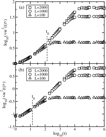
Figure 1: Time evolution of the simulated VTH width when $N=1$ for various sizes $L$. (a) Poisson deposition. (b) Uniform deposition. The initial phase for $t<t_{0}$ does not scale.

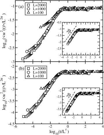
Figure 2: Scaling of the VTH width when $N=1$. (a) Poisson deposition. (b) Uniform deposition. The inserts show the data collapse for $t>t_{0}$. The slope $2\beta$ of the growth phase is consistent with $\alpha+z=2$ and $\alpha=\beta z$.

III FLAT-SUBSTRATE CONDITION

Rule $1$ $(N=1)$, is a realization of random deposition at local surface minima. As demonstrated in simulations with Poisson depositions KTN+00 , these interfaces belong to the KPZ universality class when the system size $L$ is sufficiently large. Using standard finite-size scaling techniques BS95 for $L$ of the order $10^{3}$-$10^{5}$, the scaling exponents were determined numerically to be $\beta=0.326\pm 0.005$ and $\alpha=0.49\pm 0.01$ KTN+00 . A peculiarity of this scaling, present for all $L$, is the existence of the initial phase that does not scale, as illustrated in Fig. 1a. Another feature is the lack of scaling for small $L$, approximately $L<100$. In this section we analyze the interface evolution for processes that obey rule $1$ with Poissonian, uniform and Gaussian depositions, and show that the above lack of scaling is an artifact of the flat-substrate initial condition.

Figure 1 presents typical evolutions of the interface width for moderate to large $L$ for both Poissonian and uniform depositions. A similar behavior is also seen for Gaussian depositions. A common feature is the existence of an initial growth phase, $0\leq t<t_{0}$, where the widths do not scale. For $t>t_{0}$ the widths obey the FV scaling, Eq. (2-3), with KPZ exponents. Figure 2 presents the FV scaling for Poissonian depositions (with $2\alpha=0.88$) and for uniform depositions (with $2\alpha=0.94$), both with $\alpha+z=2$, when the scaling transformation is applied for all $t\geq 0$. A similar picture of the data collapse is obtained for Gaussian depositions (with $2\alpha=0.92$). The whisker-like structures in the growth part, clearly observed in Fig. 2, demonstrate the absence of scaling for $0\leq t<t_{0}$. They vanish when the scaling is restricted to times $t\geq t_{0}$ (the inserts to Fig. 2) and full data collapse is achieved for these later times. This initial transition phase is not a finite-size effect since $t_{0}$ does not depend on $L$. For all $L$ there is one common $t_{0}$ that depends only on the deposition type. The largest $t_{0}$ is observed for the deposition with the largest variance of the random height increments $\eta$. In our examples, the smallest $t_{0}$ is for the uniform depositions (variance $1/12$) and the largest $t_{0}$ is for Poissonian depositions (variance $1$). In Gaussian depositions (variance $(1-2/\pi)$) the initial $t_{0}$ falls between these two values. Thus, while the scaling shows that the mechanism of generating correlations (i.e., rule $1$) has KPZ dynamics, the length $t_{0}$ of this initial relaxation period to KPZ scaling is not universal.

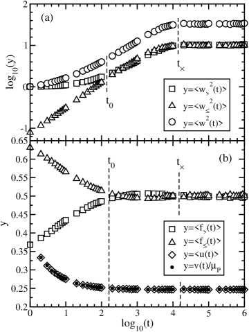
Figure 3: Time evolutions for $N=1$ with Poisson deposition $(L=1000)$. (a) The widths, $w^{2}=f_{\leq}w_{\leq}^{2}+f_{>}w_{>}^{2}$. (b) The interface velocity $v(t)$ and characteristic densities: the utilization $\langle u(t)\rangle$ ($\langle u(0)\rangle=1$, not shown), the simplex coefficients $\langle f_{>}(t)\rangle$ and $\langle f_{\leq}(t)\rangle$. The time $t_{0}$ marks the transition to the steady state (the KPZ growth), and $t_{\times}$ is the cross-over time to saturation. Here, $\mu_{P}=1$.

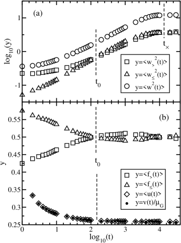
Figure 4: Time evolutions for $N=1$ with Gaussian deposition $(L=1000)$. (a) The widths, $w^{2}=f_{\leq}w_{\leq}^{2}+f_{>}w_{>}^{2}$. (b) The interface velocity $v(t)$ and characteristic densities in analogy with Fig. 3. Here, $\mu_{G}=\sqrt{2/\pi}$.

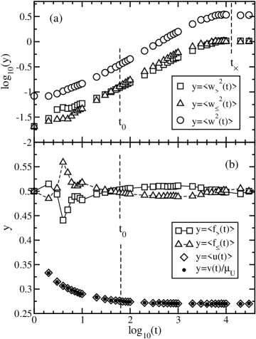
Figure 5: Time evolutions for $N=1$ with uniform deposition $(L=1000)$. (a) The widths. (b) The interface velocity $v(t)$ and characteristic densities in analogy with Fig. 3. Here, $\mu_{U}=1/2$.

The initial transition period $t_{0}$ is an artifact of the flat-substrate initial condition. To investigate it further, we write out $w^{2}(t)$ in its simplex form KNK03 as the convex linear combination

$$w^{2}(t)=f_{\leq}(t)\,w_{\leq}^{2}(t)+f_{>}(t)\,w_{>}^{2}(t),$$ (8)

where $f_{\leq}(t)+f_{>}(t)=1$ is the convex sum, i.e., $0\leq f_{\leq}(t),f_{>}(t)\leq 1$. The characteristic densities $f_{\leq}(t)$ and $f_{>}(t)$ are the fractions of sites that have their heights less-then-or-equal-to and larger-than, respectively, the mean height $\bar{h}(t)$. The corresponding widths, computed on subsets that consist of these sites alone, are $w_{\leq}^{2}(t)$ and $w_{>}^{2}(t)$, respectively. In individual simulations Eq.(8) is strictly satisfied and it is valid when averaged over many independent simulations. The convex sum is also valid for configurational averages of characteristic densities. However, Eq.(8) does not need to hold when characteristic densities and widths are changed to their corresponding configurational averages (because, in general, $\langle ab\rangle\neq\langle a\rangle\langle b\rangle$). Configurational averages of characteristic widths and densities, and the interface velocity $v(t)$ are presented in Fig. 3 for Poissonian depositions, in Fig. 4 for Gaussian depositions, and in Fig. 5 for uniform depositions. At $t=0$, the interface velocity and the utilization have their highest values $\langle u(0)\rangle=1$ because Eq. (6) is satisfied at all sites. This first step at $t=0$ is simply a random deposition step. The mean height $\bar{h}(0)=\mu$ is the mean of the distribution from which $\eta$ is sampled, which is $\mu_{P}=1$, $\mu_{G}=\sqrt{2/\pi}$ and $\mu_{U}=1/2$ for Poisson, Gaussian and uniform depositions, respectively. The fraction $f_{>}(0)$ of sites that have their heights larger than $\bar{h}(0)$ is easily computed from the corresponding distributions as the probability of selecting a site that has $h(0)$ larger than $\mu$. This gives for Poisson deposition $f_{>}(0)=\int_{\mu_{P}}^{\infty}dx\exp(-x)=1/e\approx 0.367$; for Gaussian deposition $f_{>}(0)=\sqrt{2/\pi}\int_{\mu_{G}}^{\infty}dx\exp(-x^{2}/2)=1-\mathrm{erf}(1/\sqrt{\pi})\approx 0.428$; and, for uniform deposition $f_{>}(0)=\int_{\mu_{U}}^{1}dx=1/2$. These fractions and their complements $f_{\leq}(0)=1-f_{>}(0)$ are clearly observed in Figs. 3-5. Correlations between lattice sites start to build up at $t=1$. Since initially the density $f_{\leq}(t)$ is larger than $f_{>}(t)$, depositions take place more often at sites with $h\leq\bar{h}$ then at sites with $h>\bar{h}$. This causes $f_{\leq}(t)$ to fall and $f_{>}(t)$ to rise (Figs. 3b-5b) and a faster growth of $w_{\leq}^{2}(t)$ than $w_{>}^{2}(t)$ (Figs. 3a-5a). On the average, as the density $\langle f_{>}(t)\rangle$ rises the density of local minima $\langle u(t)\rangle$ decreases. This initial evolution from the RD surface at $t=0$ to a surface with correlations at $t_{0}$ ends when $\langle f_{>}(t)\rangle\approx\langle f_{\leq}(t)\rangle\approx 1/2$. As Figs. 3-5 illustrate, at $t_{0}$ the simulations attain what we label as a steady state, one that is characterized by a constant utilization. We show in Sec. V that $v(t)$ is related to $\langle u(t)\rangle$ by a simple linear relation, hence, the steady state can be alternatively defined by a constant velocity.

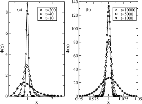
Figure 6: Poisson deposition at local surface minima for $L=1000$: distribution function $\Phi(x)$ of the interface local heights $x=h(t)/\bar{h}(t)$. (a) Early times $t\leq t_{0}$. (b) The steady state for $t>t_{0}$. Cubic-spline curves through the simulation data (symbols) are guides for the eyes. Here, $t_{0}\propto 100$.

The correlated growth phase when the scaling is observed, when $t_{0}<t\ll t_{\times}$, is characterized by a slight but noticeable excess of $\langle f_{>}(t)\rangle$ over $\langle f_{\leq}(t)\rangle$. At saturation, for $t\gg t_{\times}$, $\langle f_{>}\rangle\approx\langle f_{\leq}\rangle$. The densities $\langle f_{\leq}(t)\rangle$ and $\langle f_{>}(t)\rangle$, and the widths $\langle w_{\leq}^{2}(t)\rangle$ and $\langle w_{>}^{2}(t)\rangle$, provide the information about the height distribution $\Phi(h/\bar{h})$ of the interface local heights about the mean height $\bar{h}(t)$. It is transparent from Figs. 3-5 that for early times, $t<t_{0}$, $\Phi(h/\bar{h})$ is characterized by a positive skewness and evolves to approximately a symmetric distribution at $t_{0}$. This distribution function for Poisson depositions at local minima is presented in Fig. 6. The computation of $\Phi(x)$ is outlined in the Appendix.

The skewness of the height distribution in the stationary state of the KPZ growth has been analyzed before by den Nijs and co-workers Nijs00 ; NN97 ; CN99 for Kim-Kosterlitz models with integer step-height differences. They report that KPZ scaling is realized at times larger than a characteristic time scale that is related to slope densities. In (1+1) dimension the KPZ dynamics is characterized by zero skewness because the height distribution of the stationary state is Gaussian NN97 . In our models, the growth can be characterized alternatively either by the density of local minima (i.e., the utilization for $N=1$) that is the same as the density of local maxima KNR03 or by the density of local slopes. Since all these densities sum up to one, the constant utilization in our model is equivalent to a constant density of local slopes. Explicitly, we define the steady evolution state (or the steady state simulations) as the evolution that has the following characteristics: 1. the density of update sites is constant; and, 2. the skewness of the height distribution is approximately zero. Starting from the flat substrate, the steady growth state is achieved after the initial relaxation time $t_{0}$. In the steady state the KPZ scaling is clearly observed.

The initial time interval from $t=1$ to $t=t_{0}$ can be interpreted as the time scale over which the system retains the memory of the flat-interface initial condition. This time is a nonuniversal parameter that depends on the variance of the distribution from which the random height increment $\eta$ is sampled. The existence of this time scale accounts for the absence of universal scaling for small system sizes, even if the rule that simulates the growth represents a generic KPZ process. For KPZ dynamics the characteristic time scale on which the correlations are being built is of the order of the system size $t_{\times}\sim L^{3/2}$. If this time scale is smaller than the memory scale, $L^{3/2}<t_{0}$, the interface saturates before the simulations reach the steady state, and for such $L$ the KPZ scaling is not observed. The universal KPZ scaling is clearly observed when the system size is large enough to loose the memory of the initial condition on time scales smaller than $L^{3/2}$, i.e., when $t_{0}\ll L^{z}$.

IV SCALING ANALYSIS

In this section we analyze the interfaces generated by deposition rule $3$ that represents two simultaneously acting growth mechanisms: one is RD and the other is deposition rule $2$, both with Poisson-random height increments. First we show that rule $2$ generates KPZ correlations. Then we obtain the universal scaling function for interfaces produced by rule $3$.

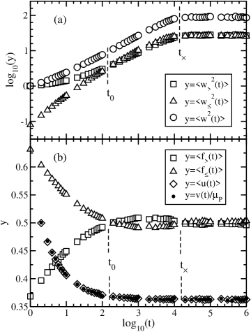
Figure 7: Time evolutions for Poisson deposition when $N=2$ and $L=1000$. (a) The widths. (b) Characteristic densities and the interface velocity, in analogy with Fig. 3.

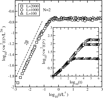
Figure 8: Scaling for $t>t_{0}$ when $N=2$. The initial relaxation period for $t<t_{0}$ is clearly noticeable in the insert that shows the widths before scaling.

Although rule $2$ allows the $k$th site to accept a deposition even if it is not a local minimum, this rule has all the essential characteristics of rule $1$, examined in Sec. III. At each time step a site must compare its local height with a local height of at least one of its immediate neighbors. As in rule $1$, deposition may not happen at a local maximum. But, since now it may happen either at a local minimum or at a local slope, the utilization of rule $2$ is larger than the one of rule $1$ (compare Fig. 3b and Fig. 7b) so the interface velocity is larger. Other than that there is no difference between these two deposition mechanisms, and the analysis presented in Sec. III for interfaces produced by rule $1$ can be restated for the interfaces that grow by rule $2$. In particular, both growths evolve on the same time scales (Fig. 7), with the initial memory scale $t_{0}\propto 100$. Figure 8 shows the scaling function for the interface widths for $t>t_{0}$, obtained with $2\alpha=0.9$ and $z=2-\alpha$, characteristic for KPZ scaling. Thus, these interfaces belong to the KPZ universality class and the scaling function is given by Eqs. (2-3). A small departure of $2\alpha$ from one, also present for $N=1$, is discussed in Sec. VI.2.

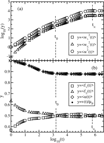
Figure 9: Time evolutions for Poisson deposition when $N=100$ and $L=1000$. (a) The widths. (b) Characteristic densities and the interface velocity, in analogy with Fig. 3 and Fig. 7.

Deposition rule $3$ produces a larger utilization than rule $2$ because now, depending on $N$, deposition at site $k$ may sometimes be accepted regardless of the relation between its local height and local heights of its neighbors. Now at each $t$, any site may increase its height, including a local maximum. Probability $p(N)$ that a site has to compare its local height with a neighbor is the probability of applying the rule $2$, which is the only mechanism that creates correlations. Alternatively, deposition at the $k$ site may happen as RD. A combination of these two deposition mechanisms produces a similar time evolution of characteristic densities and the widths as it is observed when rule $2$ is acting alone, except that now the transition to steady-state simulations and the cross-over to saturation take place on larger time scales (compare Fig. 7 and Fig. 9). In particular, the initial lack of scaling extends to $t_{0}(N)\propto t_{0}N/2$, where $t_{0}$ marks the end of the initial relaxation period in the worst-case scenario simulations. This initial relaxation time $t_{0}(N)$, when the system “remembers” the flat-interface initial condition, manifests itself in the evolution of interface widths as an early growth phase (Fig. 10) that follows the RD power law with $\beta_{1}=1/2$. The later growth phase, $t_{0}(N)\ll t\ll t_{\times}$, follows the power law with $\beta_{2}=1/3-\varepsilon$, where $\varepsilon$ is a small positive number. The evolution of the interface width can be summarized as

$$\langle w^{2}(t)\rangle\sim\left\{\begin{array}[]{r@{\quad, \quad}l}t^{2\beta_{1}}&t<t_{0}(N)\\ t^{2\beta_{2}}&t_{0}(N)\ll t\ll t_{\times}(N)\\ g(N)L^{2\alpha}&t\gg t_{\times}(N),\end{array}\right.$$ (9)

where $g(N)$ is a monotonic function of $N$. After performing scaling in $L$ of the saturated width, it appears that $g(N)$ is linear. The first growth phase is the initial relaxation when $\langle w^{2}(t)\rangle$ does not scale, therefore the following analysis is valid only for $t>t_{0}(N)$.

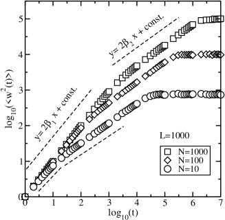
Figure 10: Two growth phases in the time evolution of the width, simulated with rule $3$ for $N>3$ and $L=1000$.

From the point of view of scaling, $\langle w^{2}(t)\rangle$ is a family of curves parametrized by $L$ and $N$. Figure 11a presents the saturated width $\langle w^{2}\rangle$ plotted against $N$ for selected values of $L$. These curves can be scaled in $L$ so as they collapse onto one curve. Figure 11b shows the scaled width $\langle w^{2}\rangle/L^{2\alpha}$, where $2\alpha=0.9$. Since $\log_{10}({\langle w^{2}\rangle/L^{2\alpha}})\sim\log_{10}{N}+\mathrm{const.}$ (dashed line in Fig. 11b), values at saturation may be further scaled in $N$, which gives the collapse to one point $\langle w^{2}\rangle/(NL^{2\alpha})\approx\mathrm{const}$. The order of scaling can be reversed, i.e., scaling in $N$ can be followed by scaling in $L$, leading to the same result. Globally, the saturated width plotted vs $(NL)$ follows a line of slope one (Fig. 11c).

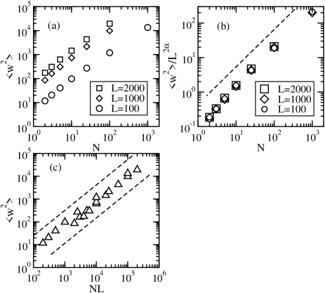
Figure 11: The saturated interface width as a two-parameter family of curves obtained in simulations with rule $3$: (a) as a function of $N$ volume elements per lattice site for several lattice sizes $L$; (b) as a function of $N$, after scaling in $L$ of the data in figure (a) (the dashed line of slope one is plotted as a reference); (c) data from figure (a) plotted vs $(NL)$ to see global trends. The data align along a straight line of the mean slope one (the dashed-line envelope).

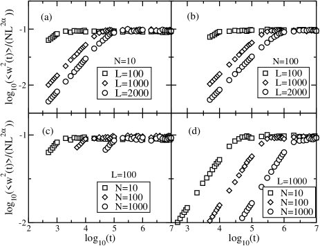
Figure 12: The steady-state evolution for $t>t_{0}$ of the scaled widths obtained with rule $3$ as a two-parameter family of curves for: (a) $N=10$; (b) $N=100$; (c) $L=100$; and, (d) $L=1000$.

Time evolution of the scaled width $\langle w^{2}(t)\rangle/(NL^{2\alpha})$ for $t>t_{0}(N)$ is displayed in Fig. 12. Here, to obtain a perfect align at saturation with the curves for $N=2$, which facilitates further scaling in $t$, we introduced a small correction such that $NL^{2\alpha}$ is multiplied by $(1\pm\varepsilon)$, where $\varepsilon$ is a small fraction (explicitly, $\varepsilon$ is the relative spread of data about the fit at saturation; the scaling is clearly seen with $\varepsilon=0$). Since the only mechanism that induces correlations in this model is deposition rule $2$, which produces surfaces from the KPZ universality class, it is expected that for each $N$ the length scales should couple with time scales via a dynamic exponent that satisfies the KPZ identity $z=2-\alpha$. Indeed, as the partial scaling in $t$ with respect to $L$ shows (Fig. 13a), this choice gives a good data collapse for each $N$ and this is not changed noticeably when $z=1.5$ is chosen. In Fig. 13a, reading from the left, the groups represent $N=2$, $N=10$, $N=100$, and $N=1000$. The last step is the scaling in $t$ with respect to $N$ of the results displayed in Fig. 13a. Here the inspection of the dilatation with $N$ of the initial $t_{0}$ proves useful since it leads to the observation that for any $L$ the initial $t_{0}(N)$ can be expressed approximately as $(N/2)t_{0}(N=1\;\mathrm{or}\;2)$. The transformation $t\to t/(N/2)$ shifts (to the left) all the curves for $N>2$ into one position. The family of curves for $N=2$ is shifted into this position when $t\to t/2$. The final result is the scaling function shown in Fig. 13b. The mean slope of the growth part is $2\beta\approx 0.58\pm 0.02$, consistent with the slope obtained for $2\alpha=0.9$ from the KPZ relation $2\beta=(2\alpha)/(2-\alpha)\approx 0.58$.

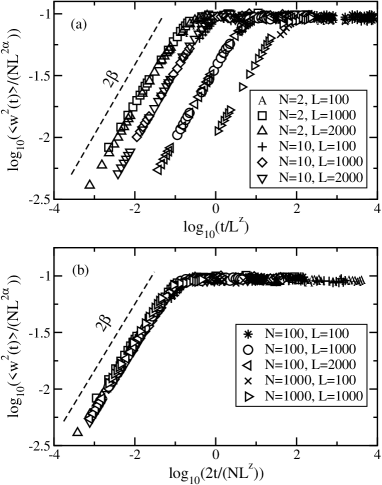
Figure 13: Scaling for the curves of Fig. 12: (a) in $t$ with respect to $L$, with the KPZ dynamic exponent $z=2-\alpha$; (b) in $t$ with respect to $N$ of the data in figure (a). Data labels displayed in the legend are common for both figures (a) and (b).

The final result, valid for $t>t_{0}(N)$, can be summarized as

$$\langle w^{2}(t)\rangle=\frac{N}{2}L^{2\alpha}f\left(\frac{2}{N}\frac{t}{L^{z}}\right),$$ (10)

where $f(y)$ satisfies Eq. (3), and $z=2-\alpha$ with $\alpha\approx 1/2$. Accordingly, the interfaces generated by the deposition/update rule $3$ belong to the KPZ universality class. In the scaling regime, the evolution can be written out explicitly as

$$\langle w^{2}(t)\rangle\sim\left\{\begin{array}[]{l@{\quad, \quad}l}(\frac{N}{2})^{1-2\beta}\,t^{2\beta}&t_{0}(N)\ll t\ll t_{\times}(N)\\ \frac{N}{2}L^{2\alpha}&t\gg t_{\times}(N),\end{array}\right.$$ (11)

where $t_{\times}(N)\sim(N/2)L^{z}$.

V INTERFACE VELOCITY

For the deposition/update models considered in this work it is possible to find the exact relation between the utilization and the interface velocity. The velocity $v(t)$ is defined as the configurational average of $\bar{v}(t)=d\bar{h}(t)/dt=(1/L)\sum_{k=1}^{L}dh_{k}(t)/dt$. Translating the update recipe to a continuum version with a continuum time-step increment $\delta t$, the update operation at site $k$ can be summarized as

$$h_{k}(t+\delta t)=\left\{\begin{array}[]{l@{\quad, \quad}l}h_{k}(t)+\delta t\,\eta_{k}(t)&\mathrm{on}\;\,\mathrm{update}\\ h_{k}(t)&\mathrm{otherwise}.\end{array}\right.$$ (12)

Substituting the above to the definition of $dh_{k}(t)/dt$ as the limit when $\delta t\to 0$, gives at $t$

$$\frac{dh_{k}(t)}{dt}=\left\{\begin{array}[]{l@{\quad, \quad}l}\eta_{k}(t)&k\;\,\mathrm{is}\;\,\mathrm{the}\;\,\mathrm{update}\;\,\mathrm{site}\\ 0&\mathrm{otherwise}.\end{array}\right.$$ (13)

In the set of $L$ sites the number of update sites is $M(t)=Lu(t)$. Since only at these sites $dh_{k}(t)/dt$ is not zero, the mean is

$$\bar{v}(t)=\frac{1}{L}\sum_{k=1}^{M(t)}\eta_{k}(t)=u(t)\frac{1}{M(t)}\sum_{k=1}^{M(t)}\eta_{k}(t).$$ (14)

Let $\mu_{P}$ be the mean of the distribution $P(\eta)$ from which $\eta_{k}$ is sampled. In the limit of $M\to\infty$, $(1/M)\sum_{k=1}^{M}\eta_{k}\to\int_{\Omega}d\eta\,\eta\,P(\eta)=\mu_{P}$. Thus, for sufficiently large $M$, the second factor in Eq. (14) is $\mu_{P}=\mathrm{const}$. Taking the configurational average of Eq. (14) gives

$$v(t)=\langle u(t)\rangle\,\mu_{P}.$$ (15)

The above derivation can be repeated for the discrete case, taking $\delta t=1$. Equation (15) is strictly satisfied by the simulation data (Figs. 3-5, 7 and 9). In simulations $\bar{v}(t)$ is computed numerically with $\delta t=1$, $\bar{v}(t)=\bar{h}(t)-\bar{h}(t-1)$, and $v(t)$ is obtained by averaging $\bar{v}(t)$ over many independent simulations.

VI DISCUSSION

In our steady-state simulations for $N>1$, the mean density of sites $p(N)=\sqrt{2/N}$ can be interpreted as the probability that at $t$ a randomly selected site followed rule $2$. The complementary density $\bar{p}=1-p$ is the probability that a randomly selected site followed RD. A similar interpretation can be given to the mean density of update sites $\langle u(t)\rangle$ as the probability that at $t$ a randomly selected lattice site increased its height; however, $\langle u(t)\rangle$ does not define a probability distribution KNR03 ; KN04 . Using a recently introduced discrete-event analytic technique for surface growth problems KNR03 ; KN04 , it is possible to derive a mean-field-like expression for the utilization $\langle u\rangle$ in the steady-state simulations. For $N\geq 2$ and $L\geq 3$ this expression KN04 is

$$\langle u\rangle=\left(1-\frac{p(N)}{2}\right)\left(1-\frac{p(N)}{4}\frac{L-1}{L}\right).$$ (16)

Because $\langle u(t)\rangle$ and $v(t)$ are related by a constant multiplicative factor $\mu_{P}$, by Eq. (15), in the scaling regime for $t>t_{0}(N)$, Eq. (16) also gives the interface velocity. However, for early times $\langle u(t)\rangle$ is unknown.

VI.1 Kinetic roughening

The scaling expressed by Eq. (10) can be written in a more general form by incorporating the probability $p=\sqrt{2/N}$. This gives

$$\langle w^{2}(t)\rangle=\left(\frac{L^{\alpha}}{p}\right)^{2}f\left(\frac{p^{2}t}{L^{z}}\right).$$ (17)

The analysis of Sec. IV can be repeated for $\langle w(t)\rangle$, which gives equivalently

$$\langle w(t)\rangle=\frac{L^{\alpha}}{p}\,f\left(\frac{p^{2}t}{L^{z}}\right).$$ (18)

The transition time to the scaling regime is $t_{0}(p)=t_{0}/p^{2}$, where $t_{0}$ marks the end of the initial non-scaling period in the case of simulations with the deposition/update rule $2$ acting alone. The cross-over time to saturation $t_{\times}$ can be read directly from Eqs. (17-18), $p^{2}t_{\times}(p)/L^{z}\approx 1$. This gives $t_{\times}(p)\approx t_{\times}/p^{2}$, where $t_{\times}$ is the saturation time when rule $2$ acts alone.

Our results for the scaling function, Eqs. (10-11) and Eqs. (17-18), are generally in accord with the work of Horowitz and Albano HA01 and Horowitz et al. HMA01 , who analyzed (1+1) dimensional two-component solid-on-solid models mixed with RD. In Ref. HA01 , the growth is simulated by ballistic deposition (of the KPZ universality class) that takes place with probability $p$ and by RD that happens with probability $(1-p)$. In Ref. HMA01 the deposition model mixes RD (taking place with probability $(1-p)$) and random deposition with surface relaxation (of the EW universality class) that takes place with probability $p$. A common characteristic of these two models and our model is the presence of two growth phases in time evolution of the interface width (Fig. 10 and Eq. (9)), where the early phase follows RD growth and this is the phase that defies the universal scaling (figures 4 in Refs. HA01 ; HMA01 ). Although this initial absence of scaling is not studied in Refs. HA01 ; HMA01 , based on our analysis of Sec. III, we infer that this early RD growth seen in Refs. HA01 ; HMA01 must be a long-time effect of some particular initial condition (not stated in HA01 ; HMA01 ) adopted in these simulations. As we showed in Sec. III, the length of this initial memory scale is a nonuniversal parameter, so comparing cross-over times to the scaling regime does not contain useful information. But, the existence of this initial memory scale and the existence of scaling for times larger than the initial relaxation time are both universal. The scaling law reported in Refs. HA01 ; HMA01 is

$$W(t,L,p)\propto\frac{L^{\tilde{\alpha}}}{p^{\delta}}\,F\left(\frac{p^{y}t}{L^{\tilde{z}}}\right),$$ (19)

where the exponents $\tilde{\alpha}$ and $\tilde{z}$ are characteristic for the universality class of the model (i.e., KPZ in HA01 and EW in HMA01 ). For the mixture of RD and random deposition with surface relaxation (the EW type model) the numerics give $\delta\approx 1$ and $y\approx 2$ HMA01 , in agreement with our findings, Eq. (18). However, for the mixture of RD and ballistic deposition (the KPZ type model) it is conjectured in HA01 that $\delta\approx 1/2$ and $y\approx 1$. In this latter scaling, although the relation between $y$ and $\delta$, $y=2\delta$, agrees with our findings, these powers are by the factor of $2$ smaller than our values. As we analyze later in this section, this difference implies that according to Ref.  HA01 the admixture of RD should affect time scales as $pt$, while our findings clearly indicate the $p^{2}t$ behavior.

The sensitivity of the surface evolution to the initial condition has been recently pointed out by Kortla et al. KPS98 in relation with phase ordering in two-component solid-on-solid models. In our modeling, to incorporate fully the dynamics of the growth, the KPZ equation should contain the mean interface velocity $v(t)$

$$h_{t}=v(t)+\nu\,h_{xx}+\frac{\lambda}{2}\,h_{x}^{2}+\zeta\,.$$ (20)

Equation (4) can be valid only for the steady-state simulations, when $v(t)=\mathrm{const}$. Therefore, it does not describe the initial dynamics at $t<t_{0}$ of our deposition models, while Eq. (20) does. Results obtained in Sec. IV, summarized by Eqs. (17-18), indicate that the admixture of the RD process (present with probability $(1-p)$ in rule $3$) elongates time scales in Eq. (20). We now scrutinize this effect from the point of view of the affine transformations involved.

Consider the following transformations that are expressed by Eqs. (17-18)

$$x\to x^{\prime}=\frac{x}{L}\,,\;\;h\to h^{\prime}=\frac{g(p)}{L^{\alpha}}h\,,\;\;t\to t^{\prime}=\frac{p^{2}}{L^{z}}t\,,$$ (21)

where $g(p)$ is to be determined (note, $g(p)$ is not independent because $x$, $h$ and $t$ are transformed simultaneously). Denoting $v=-h_{x}$, in (1+1) dimensions the convective derivative in Burger’s flow is $D_{t}v=v_{t}+\lambda\,v\,v_{x}$ BS95 . It is straightforward to show that $D_{t}v$ is invariant (up to a multiplicative factor) under transformations (21) if $\alpha+z=2$, $g(p)=p$ and if $\lambda\to\lambda^{\prime}$, $\lambda^{\prime}p^{3}=\lambda$. Then $w^{2}(t)$ transforms to $w^{\prime 2}(t^{\prime})$, $w^{\prime 2}(t^{\prime})=w^{2}(t)/(L^{2\alpha}/p^{2})\sim\Phi(t^{\prime})$ or, equivalently, $w(t)\to w(t)/(L^{\alpha}/p)~{}\sim\Phi(t^{\prime})$. This gives Eqs. (17-18). If we set $\lambda=0$ in Eq. (20) (assuming the scaling regime of constant $v(t)$), then the resulting EW equation is invariant under the same transformations providing $z=2$, $2\alpha+1=z$ and $\nu\to\nu^{\prime}$, $\nu^{\prime}p^{2}=\nu$. This, again, gives Eqs. (17-18) but with $z=2$ and $\alpha=1/2$. Transformations defined by Eq. (21) can be seen as superpositions, where the first scaling

$$x\to x/L\,,\;\;h\to h/L^{\alpha}\,,\;\;t\to t/L^{z}$$ (22)

is followed by

$$x\to x\,,\;\;h\to ph\,,\;\;t\to p^{2}t\,.$$ (23)

(The order in which transformations (22) and (23) are superimposed to form transformation (21) can be reversed.) The second transformation, defined by Eq. (23), leaves the KPZ equation (20) invariant provided that new coefficients $\nu^{\prime}$ and $\lambda^{\prime}$ are related to the old coefficients by the relations $\nu^{\prime}p^{2}=\nu$ and $\lambda^{\prime}p^{3}=\lambda$ (which is the result obtained before) and the old velocity $v(t)$ changes to a new velocity $v^{\prime}(t)=v(t^{\prime})/p$. Notice, in the absence of the RD admixture we have $p=1$ and the transformation (23) is the identity. Then transformation (21) is the usual FV scaling, Eqs. (2-3), with proper choices for $\alpha$ and $z$, depending on the process at hand (either KPZ or EW). When the RD process is present we have $p<1$. Then, inverting transformation (23) gives the changes in the local-height field $h/p$ and in time scales $t/p^{2}$. Since the elongation of the time scale is inversely proportional to $p^{2}$ this effect is more pronounced than the stretching in $h$. These phenomena take place for all $t\geq 0$ since transformation (23) is valid for all $t$, while the FV scaling or, equivalently, affine mapping given by Eq. (22) takes place only in steady-state simulations at times $t\gg t_{0}(p)$ when the system has lost the memory of the initial condition.

One possibility for the behavior seen in this paper for an admixture of the KPZ fixed point with the RD fixed point could be for a reason similar to the floating-fixed point seen in critical phenomena FFS01 ; FFS02 ; FFS03 . In that case two physical fixed points (in integer dimensions) are joined by a line of fixed points that are inaccessible (in that case in non-integer dimensions). The result is that for a finite system size, and depending on the boundary conditions involved, there is an effective critical exponent FFM01 ; FFM02 ; FFM03 ; FFM04 . Only in the limit of infinitely large systems is the physical fixed point approached. The effective critical exponents along this line of fixed points satisfy (hyper)scaling relationships, just as here the relationship $\alpha+z=2$ holds. Further investigations studying much larger systems would be needed to see if the floating-fixed point picture holds in our case where properties of both the RD and KPZ fixed points are mixed into the nonequilibrium surface model.

In summary, the only effect of the RD admixture to either a genuine KPZ or EW process is the dilatation of growth scales. The RD blending does not change the universality class of the interface since it does not change the dynamics of mechanisms that are responsible for building correlations. However, such dilatation, when combined with the initial flat-substrate condition, may obscure a clear observation of KPZ scaling in simulations as well as in experiments.

VI.2 Roughness

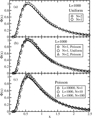
Figure 14: Distributions $\Phi(x)$ of the interface widths at saturation, $x=w^{2}/\langle w^{2}\rangle$. Results of simulations (symbols) are compared to Eq. (24) (continuous curve). (a) Uniform deposition when $L=1000$ and $N=1,2$ (binning interval $\Delta_{U}=0.05$; the data for $N=1$ fall on the top of data for $N=2$). (b) Uniform and Poisson depositions when $L=1000$ and $N=1,2$ ($\Delta_{U}=0.05$, $\Delta_{P}=0.5$). (c) Poisson deposition when $L=1000,10000$ and $N=1,10,100$ ($\Delta_{P}=1$).

In this section we discuss finite-size effects in scaling for the VTH interfaces simulated by the worst-case-scenario deposition/update rules $1$ and $2$. Despite that these interfaces belong to the KPZ universality class, the precise value of the roughness exponent depends on the lattice size $L$ and on the type of deposition. In the case of Poisson deposition it requires large $L$ to attain scaling with $2\alpha\approx 1$ KTN+00 ($\alpha$ approaches $1/2$ from below as $L$ is increased), while for uniform depositions the required $L$ is approximately two orders smaller than that for Poisson depositions.

At saturation the growth of a (1+1) dimensional KPZ (or EW) surface can be mapped onto a diffusion problem with column-height fluctuations $\delta h\sim 1/z_{w}$, where $z_{w}$ is the dynamic exponent of a random walker BS95 ; Odor04 that connects with the roughness exponent, $\alpha z_{w}=1$. The exact $\alpha=1/2$ indicates the total lack of correlations and $\alpha>1/2$ indicates their presence. The random-walk interfaces are characterized by the following width distribution function $\Phi(w^{2}/\langle w^{2}\rangle)$ FOR+94

$$\Phi(x)=\frac{\pi^{2}}{3}\sum_{n=1}^{\infty}(-1)^{n-1}n^{2}\exp\left(-\frac{\pi^{2}}{6}n^{2}x\right).$$ (24)

In simulations of growth models where $w^{2}$ depends on a single length scale, $\Phi$ is obtained by normalizing a histogram $P(w^{2})$ of the width distribution FOR+94 ; RP94 ; PRZ94 ; AR96 ; MPP+02

$$\Phi\left(\frac{w^{2}}{\langle w^{2}\rangle}\right)=\langle w^{2}\rangle P(w^{2}).$$ (25)

This technique of describing surfaces in terms of their scaling functions $\Phi$ gives very good agreement between theoretical functions $\Phi$ (whenever available) and simulated curves for growth models with integer height increments FOR+94 ; RP94 ; PRZ94 ; AR96 ; MPP+02 . Figure 14 shows $\Phi$ obtained in simulations with several $N$ and $L$ for our deposition/update models with Poisson and uniform depositions. We observe that these curves closely follow the theoretical curve given by Eq. (24). In the computation of the quantities in Eq. (25) (see Appendix) we used a variable step size $\Delta$ in binning the $w^{2}$ data ($\Delta=0.05,0.1,0.5$ and $1$) and a variable number $N_{data}$ of data points at saturation ($6.4\times 10^{6}<N_{data}<10^{8}$) to ensure that the results of Fig. 14 represent the true limit of $\Phi$ obtained in our models.

The exact collapse of the distributions $\Phi$ obtained in simulations on the theoretical curve of Fotlin et al. FOR+94 , given by Eq. (24), is not related to the type of the deposition, as is illustrated by the data in Fig. 14 and is observed even for small system sizes ($L\propto 100$). Therefore explaination for the sensitivity of $\alpha$ to $L$ and to the deposition type must lie elsewhere. For moderate to large $L$ presented in this work, when $N=1$ data collapse at saturation required $2\alpha\cong 0.94$ for uniform deposition, $2\alpha\cong 0.92$ for Gaussian deposition, and $2\alpha\cong 0.88$ for Poisson deposition. Similarly, when $N=2$ the collapse was achieved with $2\alpha\cong 0.94$ for uniform deposition and $2\alpha\cong 0.9$ for Poisson deposition. This variation of $\alpha$ with the deposition type suggest that a small departure $\delta_{\alpha}=1-2\alpha$ from the exact value $2\alpha=1$ is a nonuniversal parameter. As observed, the largest difference $\delta_{\alpha}$ is for depositions that have the largest variance (i.e., Poisson) and the smallest $\delta_{\alpha}$ is for depositions of the smallest variance (i.e., uniform). This observation strongly indicates that $\delta_{\alpha}$ is related to the system memory (introduced in Sec. III), i.e., to time scales $T$ on which the interface does not remember past depositions. In other words, $\delta_{\alpha}$ depends on the minimal interval $T$ such that, on the average, a deposition at time $t$ does not affect depositions at time $(t+T)$. Long memory scales $T$ lead to a build-up of temporal correlations, thus, produce a variation to Gaussian noise in Eq. (4), possibly modifying noise strength $D$ in Eq. (5). Such a variation may influence the way in which the system attains the stationary state Fog01 and, possibly, the value of $\alpha$. We leave this issue open to future investigations.

VI.3 False scaling

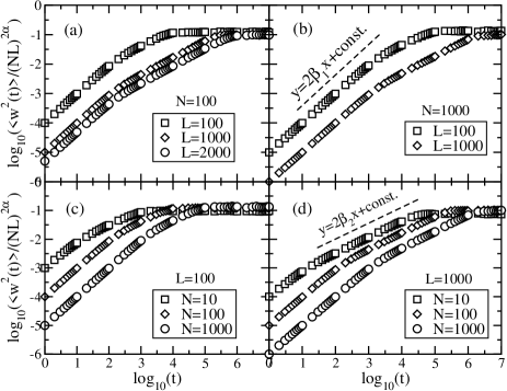
Figure 15: The false-scaling time evolution for $t>0$ of the scaled widths, obtained with Poisson depositions in rule $3$: (a) $N=100$; (b) $N=1000$; (c) $L=1000$; (d) $L=1000$.

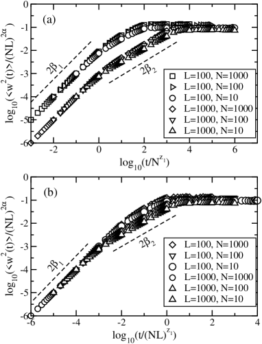
Figure 16: False scaling for the curves of Fig. 15. (a) Scaling with $N$ in $t$, $z_{1}=1$. (b) Scaling with $L$ in $t$ for the data in figure (a).

A blind application of the scaling technique to numerical data sets, without supporting analysis of temporal scales and invariants involved, may lead to false conclusions. For example, assuming a global linear behavior of $\langle w^{2}\rangle$ vs the variable $(NL)$ (Fig. 11c), it is possible to collapse the saturated widths by using an effective exponent $2\alpha\approx 1$. Performed for all $t>0$, such scaling shows two distinct growth regimes in the evolution curves (Fig. 15). For each $L$, these can be further collapsed into groups by scaling $t\to t/N^{z_{1}}$ for all $t$, taking $z_{1}=1$ (Fig. 16a). The excellent total data collapse in the first growth regime (of slope $2\beta_{1}$ in Figs. 15-16) is obtained when $t\to t/(NL)^{z_{1}}$, but at the expense of only an approximate collapse in the second growth regime (of slope $2\beta_{2}$ in Figs. 15-16). This final result (Fig. 16b) seems to look plausible because $2\beta_{1}=1$ and $2\alpha=1$ give a hypothetical exponent $z_{1}=1$, and the curves fall exactly on the top of each other in the early growth phase and at saturation. However, upon a closer inspection it appears that the length of the intermediate regime of slope $2\beta_{2}$ expands when $L$ is increased. In the limit of large but finite $L$, the scaled curves in Fig. 16b will cover the lower right-hand semi-plane, bounded by lines $y=\log_{10}(\langle w^{2}\rangle/(NL)^{2\alpha})=\mathrm{const.}$ and $y=2\beta_{1}\log_{10}(t/(NL)^{z_{1}})+\mathrm{const}$. Hence, there is no scaling. In fact, this example supports our earlier conclusion that the initial growth phase for $t<t_{0}(N)$, the artifact of the initial condition, does not scale.

VI.4 Application to PDES

In modeling of the conservative update mode in PDES, we represent sequential events on a processor in terms of their corresponding local virtual times. The column height that rises at the $k$th lattice site in the simulated VTH represents the total time of operations performed by the $k$th processor. These operations can be seen as a sequence of update cycles, where each cycle has two phases. The first phase is the processing of the assigned set of discrete events (e.g., spin flipping on the assigned sublattice). This phase is followed by a messaging phase that closes the cycle, when a processor broadcasts its findings to other processors. But the messages broadcasted by other processors may arrive any time during the cycle. Processing related to these messages (e.g., memory allocations/deallocations, sorting and/or other related operations) are handled by other algorithms that carry their own virtual times. In fact, in actual simulations, this messaging phase may take an enormous amount of time, depending on the hardware configuration and the message processing algorithms. In our modeling the time extent of the messaging phase is ignored as though communications among processors were taking place instantaneously. In this sense we model an ideal system of processors. The local virtual time of a cycle represents only the time that logical processes require to complete the first phase of a cycle. Therefore, the spread in local virtual times represents only the desynchronisation that arises due to the conservative algorithm alone.

The measure of this desynchronization is provided by $\langle w(t)\rangle$. Since in PDES the memory request per processor, required for past-state savings, is determined by the extent to which processors get desynchronized, $\langle w(t)\rangle$ can be considered as an indirect approximate measure of this memory request. Its growth during the entire time span of the PDES computations is given explicitly by Eq. (9).

We showed that in conservative PDES, given the PDES size (finite $L$ and $N$), this memory request does not grow without limit but varies as the computations evolve. The fastest growth, proportional to $\sqrt{t}$, characterizes the initial start-up phase. The length of the start-up phase depends on the load per processor (represented here by $N$). The start-up phase is characterized by decreasing values of both the utilization and the progress of the global simulated time (i.e., the smallest local virtual time from all processors at each simulation step). In the steady-state simulations, when the utilization has already stabilized at a mean constant value (and so has the progress of the global simulated time), the memory request grows slower, at a decreasing rate $\sim 1/t^{2/3}$. In this phase, the mean request can be estimated globally from Eq. (10) or Eq. (11). The important consequence of scaling, expressed by Eq. (10), is the existence of the upper bound for the memory request for any finite number $L$ of processors and for any finite load $N$ per processor. As it is stated by Eq. (11), on the average, this upper bound increases proportionally to $\sqrt{NL}$ with the size of conservative PDES.

The characteristic time scale $t_{0}(N)$ from the first step to the steady-state simulations can be estimated by monitoring the utilization for the minimal processor load (to determine $t_{0}$) and, subsequently, scaling this time with $N$. Similarly, the characteristic time scale to $t_{\times}(N)$, when the desynchronization reaches its steady state, can be scaled with the processor load to determine an approximate number of simulation steps to the point when the mean memory request does not grow anymore.

During the steady state simulations the utilization $\langle u\rangle$ is given by the approximate Eq. (16), where $p(N)=\sqrt{2/N}$. The smallest utilization $\langle u_{p}\rangle$ for any processor load is obtained by taking the limit $L\to\infty$ of Eq. (16):

$$\langle u_{p}\rangle=(1-p(N)/2)(1-p(N)/4).$$ (26)

Since as $N\to\infty$, $p(N)$ decreases as $\sim 1/\sqrt{N}$, Eq. (26) shows that $\langle u_{p}\rangle$ grows very fast when the processors’ load increases. For example, $\langle u_{p}\rangle$ for $N=100$ is about $90\%$, close to its asymptotic limit of $100\%$. For the minimal processors’ load $(p=1)$ Eq. (16) gives for $L\geq 3$

$$\langle u_{0}\rangle=\frac{3}{8}+\frac{1}{8L}.$$ (27)

In the limit $L\to\infty$, $\langle u_{0}\rangle$ is the smallest possible value of the utilization. As Eq. (27) shows, this value is a non-zero constant (equal to $3/8$ when derived from simulations with Poissonian distribution of waiting times). This nonzero lower bound on the utilization and the finite upper bound for the memory request for finite $L$ show that conservative PDES are generally scalable with the number of computing processors when performed in the ring communication topology. The extension of this conclusion to other communication topologies requires a separate study.

VII SUMMARY AND CONCLUSIONS

We considered a two-component growth in (1+1) dimensions. One of the components is RD that takes place with probability $(1-p)$. The other component, which takes place with probability $p$, is a deposition process that generates correlations typical of KPZ dynamics. The growth is simulated from an initially flat substrate.

We show that the flat-substrate initial condition is responsible for the existence of the initial non-scaling regime in simulations. The length of this initial phase is a nonuniversal parameter (it depends on the type of depositions and on the particulars of the model). However, its presence is a universal phenomenon.

During the initial phase the simulations relax to a steady state. For the models considered in this work, the transition time to the steady state can be defined as the time when the mean interface velocity attains a constant value. We showed that for these models the mean interface velocity is a multiple of the mean utilization.

During the steady state the interface width satisfies FV scaling. We derived the universal scaling function for the width and showed that the RD admixture acts as a dilatation mechanism to the time and height scales, but leaves the KPZ correlations intact. This conclusion has been generalized to two-component models that mix RD with depositions that classify within the EW universality class. In particular, we showed that the RD admixture is responsible for the $p$ dependent affine change of scales ($h\to h/p$ and $t\to t/p^{2}$) that is superimposed on the usual scaling and leaves the dynamics invariant.

The models, studied in this work, that give rise to the KPZ correlations are the Poisson-, the Gauss-, and the uniform-random depositions either to local interface minima or to local minima and randomly selected local slopes. Despite that the simulated interfaces belong to the KPZ universality class, the precise value of their roughness exponent depends on the deposition type. This observation suggests that such noisy deposition mechanisms may produce relatively long-scale temporal correlations. Secondly, this small departure from the exact value is nonuniversal. Further studies are required to investigate this issue.

In application to conservative PDES, we showed that the memory request per processor, required for state savings, does not grow without limit for a finite number of processors and a finite load per processor but varies as the PDES evolve. The important consequence of the derived scaling is the existence of the upper bound for the desynchronization, thus, for this memory request. Also, the utilization of the parallel processing environment has a non-zero lower bound as the number of processors increases infinitely. Thus, the conservative PDES are generally scalable in the ring communication topology.

*

Appendix A Distributions

Both $h_{k}(t)$ and $w^{2}(t)$ are real numbers that take on continuous values. Suppose $S=\{f_{1},f_{2},...,f_{N}\}$ is a set of $N$ such numbers obtained in simulations. Let $a=\min(S)$ and $b=\max(S)$. The interval $(b-a)$ is partitioned into $M$ segments, each of length $\Delta=(b-a)/M$. Each segment is a bin that is indexed by its left end $y_{i}=a+(i-1)\Delta$, $i=1,2,...,M$. Let $m_{i}$ be the multiplicity of the $i$th bin, i.e., $m_{i}$ is the number of points from $S$ that fall between $y_{i}$ and $y_{i+1}$. The mean value of $S$ is $\langle f\rangle=1/N\sum_{k=1}^{N}f_{k}=\sum_{i=1}^{M}P_{i}\,\langle f_{i}\rangle$, where $\langle f_{i}\rangle=(1/m_{i})\sum_{n=1}^{m_{i}}f_{in}$ is the mean value taken on a subset of $S$ that belongs to the $i$th bin, and $P_{i}$ is the frequency function $P_{i}=(m_{i}/N)(1/\Delta)$. The abscissas $x_{i}$ and function values $\Phi_{i}=\Phi(x_{i})$ are: $x_{i}=\langle f_{i}\rangle/\langle f\rangle$ and $\Phi_{i}=\langle f\rangle P_{i}$. These values are plotted in Fig. 6 and Fig. 14. Here, $\Phi(x)$ is properly normalized $\int_{0}^{\infty}dx\,\Phi(x)=1$. The absolute spread $(b-a)$ determines a suitable $\Delta$ in the computation of $\langle f_{i}\rangle$ within acceptable precision. This gives the total number $M$ of bins. For a given $M$, the accuracy of $P_{i}$ depends on $N$.

References

- (1) F. Family and T. Vicsek, J. Phys. A 18, L75 (1985).
- (2) M. Kardar, G. Parisi, and Y.-C. Zhang, Phys. Rev. Lett. 56, 889 (1986).
- (3) A.-L. Barabasi and H. E. Stanley, Fractal Concepts in Surface Growth (Cambridge University Press, Cambridge, 1995).
- (4) S. F. Edwards and D. R. Wilkinson, Proc. R. Soc. London A 381, 17 (1982).
- (5) J. Krug, Adv. Phys. 46, 139 (1997).
- (6) H. N. Yang, G.-C. Wang, and T. M. Lu, Diffraction from Rough Surfaces and Dynamic Growth Fronts (World Scientific, Singapore, 1993).
- (7) F. Family and T. Viscek, eds., Dynamics of Fractal Surfaces (World Scientific, Singapore, 1991).
- (8) M. Kardar, in Proceedings of the 4h International Conference on Surface X-Ray and Neutron Scattering, edited by G. P. Felcher and H. You, Physica B 221, 60 (1996).
- (9) G. Odor, Rev. Mod. Phys. 76, XX (2004).
- (10) S. Das Sarma, C. J. Lanczycki, R. Kotlyar, and S. V. Ghaisas, Phys. Rev. E 53, 359 (1996).
- (11) C. Dasgupta, S. Das Sarma, and J. M. Kim, Phys. Rev. E 54, R4552 (1996).
- (12) J. M. Lopez and J. Schmittbuhl, Phys. Rev. E 57, 6405 (1998).
- (13) S. Morel, J. Schmittbuhl, J. M. Lopez, and G. Valentin, Phys. Rev. E 58, 6999 (1998).
- (14) J. M. Lopez and M. A. Rodriguez, Phys. Rev. E 54, R2189 (1996).
- (15) A. Bru, J. M. Pastor, I. Fernaud, I. Bru, S. Melle, and C. Berenguer, Phys. Rev. Lett. 81, 4008 (1998).
- (16) R. Cuerno and M. Castro, Phys. Rev. Lett. 87, 236103 (2001).
- (17) H. C. Fogedby, J. Phys.: Cond. Mat. 14, 1557 (2002).
- (18) G. Fotlin, K. Oerding, Z. Racz, R. L. Workman, and R. K. Zia, Phys. Rev. E 50, R639 (1994).
- (19) J. G. Amar and F. Family, Phys. Rev. A 41, 3399 (1990).
- (20) J. G. Amar and F. Family, Phys. Rev. A 45, R3373 (1992).
- (21) T. Hwa and E. Frey, Phys. Rev. A 44, R7873 (1991).
- (22) T. Nattermann and L.-H. Tang, Phys. Rev. A 45, 7156 (1992).
- (23) R. A. Blythe and M. R. Evans, Phys. Rev. E 64, 051101 (2001).
- (24) Y. P. Pellegrini and R. Jullien, Phys. Rev. A 43, 920 (1991).
- (25) A. Chame and F. D. A. Aaeao Reis, Phys. Rev. E 66, 51104 (2002).
- (26) A. Hernandez-Machado, J. Soriano, A. M. Lacasta, M. A. Rodriguez, L. Ramirez-Piscina, and J. Ortin, Europhys. Lett. 55, 194 (2001).
- (27) J. Soriano, J. Ortin, and A. Hernandez-Machado, Phys. Rev. E 66, 031603 (2002).
- (28) J. Soriano, J. Ortin, and A. Hernandez-Machado, Phys. Rev. E 67, 056308 (2003).
- (29) G. M. Foo and R. B. Pandey, Phys. Rev. Lett. 80, 3767 (1998).
- (30) F. Bentrem, R. B. Pandey, and F. Family, Phys. Rev. E 62, 914 (2000).
- (31) M. D. Grynberg, Phys. Rev. E 68, 041603 (2003).
- (32) M. Kotrla, M. Predota, and F. Slanina, Surf. Sci. 402, 249 (1998).
- (33) M. Kotrla, F. Slanina, and M. Predota, Phys. Rev. B 58, 10003 (1998).
- (34) W. Wang and H. Cerdeira, Phys. Rev E 47, 3357 (1993).
- (35) H. F. El-Nashar and H. A. Cerdeira, Phys. Rev. E 61, 6149 (2000).
- (36) F. D. A. Aarao Reis, Phys. Rev. E 66, 027101 (2002).
- (37) C. M. Horowitz, R. A. Monetti, and E. Albano, Phys. Rev. E 63, 066132 (2001).
- (38) C. M. Horowitz and E. V. Albano, J. Phys. A: Math. Gen. 34, 357 (2001).
- (39) T. J. da Silva and J. G. Moreira, Phys. Rev. E 63, 041601 (2001).
- (40) J. M. Kim and J. M. Kosterlitz, Phys. Rev. Lett. 62, 2289 (1989).
- (41) R. M. Fujimoto, Parallel and Distributed Simulation Systems (John Wiley and Sons, Inc., New York, 2000).
- (42) K. M. Chandy and J. Misra, IEEE Trans. Software. Eng. 5, 440 (1979).
- (43) R. Fujimoto, Commun. ACM 33, 30 (1990).
- (44) J. Misra, ACM Comput. Surv. 18, 39 (1986).
- (45) B. D. Lubachevsky, Complex Syst. 1, 1099 (1987).
- (46) B. D. Lubachevsky, J. Comp. Phys. 75, 103 (1988).
- (47) D. A. Jefferson, ACM Trans. Programming Languages Syst. 7, 404 (1985).
- (48) P. M. Dickens and P. F. Reynolds, in Proceedings of the SCS Multiconference on Distributed Simulation, San Diego, edited by D. Nicol and R. Fujimoto, Simulation Series Vol. 22, pp. 161-164 (1990).
- (49) J. S. Steinman, in Proceedings of the Seventh workshop on Parallel and Distributed Simulation, edited by R. Bagrodia and D. Jefferson (IEEE Computer Society Press, Los Alamitos, CA, 1993), p. 109.
- (50) B. D. Lubachevsky, V. Privman, and S. C. Roy, J. Comput. Phys. 126, 152 (1996).
- (51) G. Korniss, M. A. Novotny, and P. A. Rikvold, Comput. Phys. 153, 488 (1999).
- (52) G. Korniss, C. J. White, P. A. Rikvold, and M. A. Novotny, Phys. Rev. E 63, 016120 (2001).
- (53) G. Korniss, P. A. Rikvold, and M. A. Novotny, Phys. Rev. E 66, 056127 (2002).
- (54) P. M. A. Sloot, B. J. Overeiner, and A. Schoneveld, Comp. Phys. Comm. 142, 76 (2001).
- (55) B. J. Overeiner, A. Schoneveld, and P. M. Sloot, in Parallel and Distributed Discrete Event Simulation, edited by C. Tropper (Nova Science Publishers, Inc, New York, 2002) p. 79.
- (56) G. Korniss, Z. Toroczkai, M. A. Novotny, and P. A. Rikvold, Phys. Rev. Lett. 84, 1351 (2000).
- (57) A. Kolakowska, M. A. Novotny, and P. A. Rikvold, Phys. Rev. E 68, 046705 (2003).
- (58) A. Kolakowska and M. Novotny, Phys. Rev. B 69, 075407 (2004).
- (59) G. Korniss, M. A. Novotny, A. Kolakowska, and H. Guclu, in Proceedings of the 2002 ACM Symposium on Applied Computing (ACM, Inc., 2002), p.132.
- (60) A. Kolakowska, M. A. Novotny, and G. Korniss, Phys. Rev. E 67, 046703 (2003).
- (61) G. Korniss, M. A. Novotny, H. Guclu, Z. Toroczkai, and P. A. Rikvold, Science 299, 677 (2003).
- (62) M. A. Novotny, A. Kolakowska, and G. Korniss, in The Monte Carlo Method in the Physical Sciences, edited by J. E. Gubernatis (AIP Publishing, New York, 2003), p. 240.
- (63) M. den Nijs, APCTP Bulletin 6 (2000).
- (64) M. den Nijs and J. Neergaard, J. Phys A 30, 1935 (1997).
- (65) C.-S. Cin and M. den Nijs, Phys. Rev. E 59, 2633 (1999).
- (66) D. O’Connor and C.R. Stephens, Nucl. Phys. B360, 297 (1991).
- (67) D. O’Connor and C.R. Stephens, J. Phys. A 25, 101 (1992).
- (68) D. O’Connor and C.R. Stephens, Int. J. Mod. Phys. C A9, 2805 (1994).
- (69) M.A. Novotny, Phys. Rev. Lett. 70, 109 (1993).
- (70) M.A. Novotny, Phys. Rev. B 46, 2939 (1992).
- (71) M.A. Novotny, Int. J. Mod. Phys. C 7, 361 (1996).
- (72) M.A. Novotny, Europhys. Lett. 17, 297 (1992); erratum 18 92(E) (1992).
- (73) Z. Racz and M. Plischke, Phys. Rev. E 50, 3530 (1994).
- (74) M. Plishke, Z. Racz, and R. K. P. Zia, Phys. Rev. E 50, 3589 (1994).
- (75) T. Antal and Z. Racz, Phys. Rev. E 54, 2256 (1996).
- (76) E. Marinari, A. Pagnani, G. Parisi, and Z. Racz, Phys. Rev. E 65, 026136 (2002).
- (77) H. C. Fogedby, Europhys. Lett. 56, 492 (2001).