Also at: ]Department of Physics and State Key Laboratory for Mesoscopic Physics, Peking University, Beijing 100871, China.

The Spin Mass of an Electron Liquid

Abstract

We show that in order to calculate correctly the spin current carried by a quasiparticle in an electron liquid one must use an effective “spin mass” $m_{s}$, that is larger than both the band mass, $m_{b}$, which determines the charge current, and the quasiparticle effective mass $m^{*}$, which determines the heat capacity. We present microscopic calculations of $m_{s}$ in a paramagnetic electron liquid in three and two dimensions, showing that the mass enhancement $m_{s}/m_{b}$ can be a very significant effect.

The recent explosion of interest in metal and semiconductor spintronics Wolf ; Awschalom has brought into sharp focus the basic problem of calculating the spin current carried by a nonequilibrium electronic system. The standard approach is to solve the Boltzmann equation for the nonequilibrium distribution function; but this is not sufficient when many-body effects due to electron-electron interactions need to be taken into account. In fact, electronic correlations are particularly strong in low-dimensional systems, such as magnetic semiconductor films and wires, which are currently being considered for the realization of spin transistors Ruster03 . One might hope to take care of the many-body effects by solving, instead of the Boltzmann equation, the Landau-Silin transport equation for quasiparticles NP . But even this is not sufficient, since the transport equation per se does not tell us how to connect the quasiparticle distribution function to the spin-current. The key question, which seems to have been overlooked so far in the growing literature on spin transport zhangrashba , is also a very basic one, namely, what is the spin-current carried by a single quasiparticle of momentum $\vec{p}$ and spin $\sigma$? Without knowing the answer to this question it is not possible to calculate the spin current from first-principles. In this paper we show that, in order to calculate the spin current correctly, one must recognize that the effective spin mass $m_{s}$, which determines the relation between the spin current and the quasiparticle momentum, is neither the band mass $m_{b}$ (which controlls the charge current), nor the quasiparticle mass $m^{*}$ (which controls the heat capacity), but rather a new many-body quantity, controlled by spin correlations. Our calculations show that the spin mass, in spite of uncertainties due to the approximate character of the many-body theory, can be considerably larger than the bare band mass in a two-dimensional electron gas (by contrast, the quasiparticle effective mass is typically very close to the band mass). Hence, the spin mass will have to be taken into account whenever a quantitative comparison between theory and experiment is desired.

Let us begin by describing the physical origin of the spin mass. The spin current, $\vec{j}_{s}=\vec{j}_{\uparrow}-\vec{j}_{\downarrow}$, is defined as the difference of the up-spin and down-spin currents, $\vec{j}_{\uparrow}$ and $\vec{j}_{\downarrow}$, which in turn are defined as the expectation values of the operators

$$\hat{\vec{j}}_{\sigma}=\sum_{i=1}^{N}\frac{\hat{\vec{p}}_{i}}{m_{b}}\frac{1+\sigma\hat{\sigma}_{z,i}}{2}~{}$$ (1)

in the appropriate nonequilibrium state. Here $\sigma=1$ for $\uparrow$ spins and $\sigma=-1$ for $\downarrow$ spins, $m_{b}$ is the bare band mass, $\hat{\vec{p}}_{i}$ is the canonical momentum operator of the $i$-th electron, $\hat{\sigma}_{z,i}$ is the Pauli matrix of the $z$-component of the spin of the $i$-th electron, $\frac{1+\sigma\hat{\sigma}_{i,z}}{2}$ is the projector on the $\sigma$-spin component of the $i$-th electron, and $N$ is the number of electrons. Let us consider a many-body state, denoted by $|\vec{p}\sigma\rangle$, which contains a single quasiparticle of momentum $\vec{p}$ and spin $\sigma$. This state carries a total current $\vec{j}=\frac{\vec{p}}{m_{b}}$, whether or not interactions are taken into account. The reason why this is so is simply that the state $|\vec{p}\sigma\rangle$, which contains a quasiparticle of momentum $\vec{p}$ and spin $\sigma$, is an eigenstate of the current operator $\hat{\vec{j}}=\sum_{i=1}^{N}\frac{\hat{\vec{p}}_{i}}{m_{b}}$ with eigenvalue $\frac{\vec{p}}{m_{b}}$. As a consequence, the current density associated with the distribution $n_{\sigma}(\vec{r},\vec{p},t)$ is given by footnote2

$$\vec{j}(\vec{r},t)=\sum_{\vec{p}\sigma}\frac{\vec{p}}{m_{b}}n_{\sigma}(\vec{r},\vec{p},t)~{}.$$ (2)

The difficulty in calculating the spin current arises from the fact that the state $|\vec{p}\sigma\rangle$ is not an eigenstate of $\hat{\vec{j}}_{\uparrow}$ or $\hat{\vec{j}}_{\downarrow}$: thus, we cannot automatically say that in this state $\vec{j}_{\sigma}=\frac{\vec{p}}{m_{b}}$ and $\vec{j}_{-\sigma}=0$, even though these expectation values would be consistent with the total value of $\vec{j}$. All we can say, a priori, is that the expectation values of $\hat{\vec{j}}_{\uparrow}$ and $\hat{\vec{j}}_{\downarrow}$ in the state $|\vec{p}\sigma\rangle$ must be proportional to $\vec{p}$ and add up to $\frac{\vec{p}}{m_{b}}$. Thus, we write

$$\langle\vec{p}\sigma|\hat{\vec{j}}_{\tau}|\vec{p}\sigma\rangle=\alpha_{\tau\sigma}\frac{\vec{p}}{m_{b}}~{},$$ (3)

where $\alpha_{\tau\sigma}$ is a $2\times 2$ matrix whose columns add up to $1$, so that the total current is $\frac{\vec{p}}{m_{b}}$. Notice that in a paramagnetic system $\alpha_{\uparrow\uparrow}=\alpha_{\downarrow\downarrow}$, and, therefore $\alpha_{\uparrow\downarrow}=\alpha_{\downarrow\uparrow}$: for simplicity’s sake, we will focus on just this case from now on. The above Eq. (3) implies that the spin current carried by an up-spin quasiparticle of momentum $\vec{p}$ is

$$\vec{j}_{s}(\vec{p}\uparrow)=(\alpha_{\uparrow\uparrow}-\alpha_{\downarrow\uparrow})\frac{\vec{p}}{m_{b}}~{}\equiv\frac{\vec{p}}{m_{s}}~{},$$ (4)

and, similarly, the spin-current carried by a down-spin quasiparticle is

$$\vec{j}_{s}(\vec{p}\downarrow)=(\alpha_{\uparrow\downarrow}-\alpha_{\downarrow\downarrow})\frac{\vec{p}}{m_{b}}~{}\equiv-\frac{\vec{p}}{m_{s}}~{},$$ (5)

since $\alpha_{\uparrow\uparrow}=\alpha_{\downarrow\downarrow}$. These equations define a spin mass $m_{s}$, which controls the spin current in much the same way as $m_{b}$ controls the charge current footnote3 .

Combining Eqs. (4) and  (5) we see that the correct expression for the spin current density carried by a nonequilibrium quasiparticle distribution $n_{\sigma}(\vec{r},\vec{p},t)$ is

$$\vec{j}_{s}(\vec{r},t)=\sum_{\vec{p}}\frac{\vec{p}}{m_{s}}\left[n_{\uparrow}(\vec{r},\vec{p},t)-n_{\downarrow}(\vec{r},\vec{p},t)\right]~{}.$$ (6)

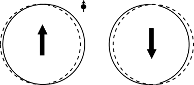
Figure 1: Spin-momentum separation in a Fermi liquid: the momentum of an up-spin quasiparticle resides, in part, with down-spin particles. The solid lines represent the Fermi surfaces and the dashed lines indicated the collective shifts in the momentum distribution of up- and down- spins.

It is clear that $m_{s}$ must be larger than $m_{b}$ since $\alpha_{\uparrow\uparrow}$ and $\alpha_{\uparrow\downarrow}$ are positive numbers that add up to $1$, implying that $\alpha_{\uparrow\uparrow}-\alpha_{\downarrow\uparrow}<1$. The positivity of $\alpha_{\uparrow\uparrow}$ and $\alpha_{\uparrow\downarrow}$ can be intuitively grasped by considering the physical picture illustrated in Figure 1. We start from an exact eigenstate of the noninteracting system with full Fermi spheres of up- and down-spins and an additional single particle of momentum $\vec{p}$ and spin $\uparrow$ out of the Fermi sphere. In this state $\vec{j}_{\uparrow}=\frac{\vec{p}}{m_{b}}$ and $\vec{j}_{\downarrow}=0$. The quasiparticle state is now obtained by slowly turning on the electron-electron interaction. The total momentum and spin do not change in the process, but some momentum is transferred from the up- to the down-spin component of the liquid: one may say that the up-spin quasiparticle drags along some down-spin electrons as part of its “screening cloud”. As a result, the magnitude of $\vec{j}_{\uparrow}$ is smaller than $\frac{\vec{p}}{m_{b}}$ by an amount equal to ${\vec{j}}_{\downarrow}$. The magnitude of the spin current is a fortiori smaller than $\frac{\vec{p}}{m_{b}}$, which implies $m_{s}>m_{b}$. Notice that the “spin-momentum separation” described above is entirely due to correlations between electrons of opposite spin orientation. Interactions between same-spin electrons do not contribute to this effect.

Having thus clarified the general concept of the spin mass we now proceed to (1) relate $m_{s}$ to the quasiparticle effective mass and the Landau Fermi liquid parameters, (2) relate $m_{s}$ to the small wave vector and low frequency limit of the spin local field factor $G_{-}(q,\omega)$, and (3) present approximate microscopic calculations of $m_{s}$ in a paramagnetic electron liquid in three and two dimensions.

Let us start from the quasiparticle state $|\vec{p}\sigma\rangle$ and apply to it the unitary transformation $\hat{U}=\exp\left[i\sum_{i,\tau}\vec{q}_{\tau}\cdot\vec{r}_{i}\frac{1+\tau\hat{\sigma}_{z,i}}{2}\right]$, which boosts the momenta of the $\tau$-spin electrons by $\vec{q}_{\tau}$. By applying $\hat{U}$ to the fundamental hamiltonian of the electron liquid one can straightforwardly show that the change in energy of any state, to first order in $\vec{q}_{\sigma}$, is

$$\Delta E=\sum_{\tau}\vec{j}_{\tau}\cdot\vec{q}_{\tau}~{}.$$ (7)

On the other hand, for the quasiparticle state under consideration, we know that $\vec{j}_{\tau}=\alpha_{\tau\sigma}\frac{\vec{p}}{m_{b}}$. Substituting this into Eq. (7) we get

$$\Delta E=\sum_{\tau}\alpha_{\tau\sigma}\frac{\vec{p}\cdot\vec{q}_{\tau}}{m_{b}}~{}.$$ (8)

The energy change under this transformation can also be calculated with the help of the Landau theory of Fermi liquids. There are two contributions: one from the boost in the momentum of the quasiparticle, and the other from the collective displacement of the Fermi surfaces by $\vec{q}_{\tau}$. A standard calculation gives

$$\Delta E=\sum_{\tau}\biggl{\{}\frac{\vec{p}}{m^{*}}\delta_{\sigma\tau}-\sum_{\vec{p}^{\prime}}f_{\vec{p}\sigma,\vec{p}^{\prime}\tau}\vec{\nabla}_{\vec{p}^{\prime}}n_{0,\tau}({\vec{p}^{\prime}})\biggr{\}}\cdot{\vec{q}}_{\tau}~{},$$ (9)

where $n_{0,\tau}(\vec{p})=\Theta(p_{F}-p)$ is the momentum distribution in the ground state and $p_{F}$ is the Fermi momentum.

Comparing Eqs. (8) and (9), we arrive at the identifications

$$\alpha_{\uparrow\uparrow} = \frac{m_{b}}{m^{*}}\left[1+\frac{F_{1}^{\uparrow\uparrow}}{2d}\right]~{},$$

$$\alpha_{\uparrow\downarrow} = \frac{m_{b}}{m^{*}}\frac{F_{1}^{\uparrow\downarrow}}{2d}~{},$$ (10)

where $d$ is the number of spatial dimensions and $F_{\ell}^{\sigma\tau}\equiv N^{*}(0)\int\frac{d\Omega}{4\pi}f_{\vec{p}\sigma,\vec{p}^{\prime}\tau}P_{\ell}(\cos\theta)$ is the angular average of the interaction function, weighted with the Legendre polynomial $P_{\ell}(\cos\theta)$ (or just $\cos\ell\theta$ in two dimensions) and multiplied by the density of states at the Fermi surface, $N^{*}(0)$. Notice that the sum rule $\sum_{\tau}\alpha_{\tau\sigma}=1$ is satisfied by virtue of the well known Fermi liquid relation NP

$$\frac{m_{b}}{m^{*}}=\frac{1}{1+F_{1}^{s}/d}~{},$$ (11)

where $F_{\ell}^{s(a)}=\frac{1}{2}\left[F_{\ell}^{\uparrow\uparrow}+(-)F_{\ell}^{\uparrow\downarrow}\right]$ are the standard dimensionless Landau parameters defined, for example, in Ref. NP . The spin mass, on the other hand, is given by (see Eq. (4))

$$\frac{m_{s}}{m^{*}}=\frac{1}{1+F_{1}^{a}/d}~{},$$ (12)

showing that the relation of $m_{s}$ to $m^{*}$ is to the spin-channel what the relation of $m_{b}$ to $m^{*}$ is to the density channel.

It should be noted that the spin current density obtained from Eq. (6) satisfies the continuity equation

$$\frac{\partial}{\partial t}n_{s}(\vec{r},t)+\vec{\nabla}\cdot\vec{j}_{s}(\vec{r},t)=0~{},$$ (13)

where $n_{s}({\vec{r}},t)=n_{\uparrow}({\vec{r}},t)-n_{\downarrow}({\vec{r}},t)$, is the spin density. Conversely, Eq. (12) could have been directly obtained from the requirements of charge and spin conservation.

The microscopic calculation of Landau parameters is notoriously difficult. Diagrammatic calculations of $F_{1}^{s}$ and $F_{1}^{a}$ in the three-dimensional electron liquid were done by Yasuhara and Ousaka yasuhara , and the calculated parameters, together with the resulting values of $m_{s}/m_{b}$ are listed in the upper half of Table 1 for various values of the Wigner-Seitz radius $r_{s}$. In two dimensions the parameters $F_{1}^{s}$ and $F_{1}^{a}$ were calculated by a variational Quantum Monte Carlo method in Ref. kwon . The parameters and the resulting values of $m_{s}/m_{b}$ are listed in the bottom half of Table 1. Notice that the spin mass enhancement in two dimensions is considerably higher than in three dimensions.

$d$	$r_{s}$	$1$	$2$	$3$	$4$	$5$
$3$	$\frac{F_{1}^{s}}{d}~{}$	-0.0543	-0.0647	-0.0713	-0.0773	-0.0829
	$\frac{F_{1}^{a}}{d}~{}$	-0.0645	-0.0825	-0.0915	-0.0956	-0.0965
	$\frac{m_{s}}{m_{b}}~{}$	1.011	1.019	1.022	1.020	1.015
$2$	$\frac{F_{1}^{s}}{d}~{}$	-0.071	-0.050	-0.015	–	0.061
	$\frac{F_{1}^{a}}{d}~{}$	-0.096	-0.120	-0.130	–	-0.136
	$\frac{m_{s}}{m_{b}}~{}$	1.028	1.080	1.132	–	1.228

Table 1: Landau parameters from Refs. yasuhara and kwon and spin mass enhancement $\frac{m_{s}}{m_{b}}=\frac{1+F_{1}^{s}/d}{1+F_{1}^{a}/d}$ in the d-dimensional electron liquid.

In view of the uncertainty in the calculation of the Landau parameters it seems worthwhile to attempt another kind of calculation, which does not rely on diagrammatic expansions. We first establish the connection between the spin mass and the dynamical local field factor in the spin channel. We recall that the dynamical spin susceptibility of an electron liquid is usually represented in the form

$$\chi_{s}(q,\omega)=\frac{\chi_{0}(q,\omega)}{1+v_{q}G_{-}(q,\omega)\chi_{0}(q,\omega)}~{},$$ (14)

where $\chi_{0}(q,\omega)$ is the noninteracting spin susceptibility (i.e., the Lindhard function), $v_{q}$ is the Fourier transform of the Coulomb interaction ($=4\pi e^{2}/q^{2}$ in three dimensions and $2\pi e^{2}/q$ in two dimensions) and $G_{-}(q,\omega)$ is the dynamical local field factor in the spin channel. In the limit $q\to 0$ and small, but finite frequency ($\omega\ll\epsilon_{F}/\hbar$ where $\epsilon_{F}$ is the Fermi energy), Eq. (14) reduces to

$$\chi_{s}(q,\omega)\stackrel{{\scriptstyle q\to 0}}{{\to}}\frac{nq^{2}}{m_{b}\left[1+\lim_{q\to 0}\frac{nq^{2}v_{q}G_{-}(q,\omega)}{m_{b}\omega^{2}}\right]\omega^{2}}~{}.$$

On the other hand, the small-$q$/finite-$\omega$ limit of $\chi_{s}(q,\omega)$ can also be calculated by solving the kinetic equation NP in the presence of slowly varying external fields $V_{\sigma}(q,\omega)$. In this region collisions are irrelevant, and one gets the spin response

$$\delta n_{s}(\vec{q},\omega)\simeq\frac{nq^{2}}{m_{s}\omega^{2}}~{}V_{s}(\vec{q},\omega)~{},$$ (16)

where $\delta n_{s}(\vec{q},\omega)=\delta n_{\uparrow}(\vec{q},\omega)-\delta n_{\downarrow}(\vec{q},\omega)$ and $V_{s}(\vec{q},\omega)=[V_{\uparrow}(\vec{q},\omega)-V_{\downarrow}(\vec{q},\omega)]/2$. Therefore,

$$\chi_{s}(q,\omega)\stackrel{{\scriptstyle q\to 0}}{{\to}}\frac{nq^{2}}{m_{s}\omega^{2}}~{}.$$ (17)

Comparing the above equation with Eq. (The Spin Mass of an Electron Liquid) leads to the identification

$$\frac{m_{s}}{m_{b}}=1+\lim_{\omega\to 0}\lim_{q\to 0}\frac{nq^{2}v_{q}G_{-}(q,\omega)}{m_{b}\omega^{2}}~{}.$$ (18)

The order of the limits is, of course, essential. When $\omega$ tends to zero first, $G_{-}(q,\omega)$ vanishes as $q^{d-1}$ for $q\to 0$, so as to yield a finite enhancement of the uniform static spin susceptibility. In Eq. (18), however, $q$ tends to zero first, and we see that $v_{q}G_{-}(q,\omega)$ must go as $\frac{\omega^{2}}{q^{2}}$ in order to give a finite value of the spin mass.

The above analysis, combined with the Kramers-Krönig dispersion relation, leads to the following relation between the real and the imaginary part of $G_{-}(q,\omega)$:

$$\lim_{q\to 0}\Re eG_{-}(q,\omega)=\lim_{q\to 0}\frac{2}{\pi}{\cal P}\int_{0}^{\infty}d\omega^{\prime}~{}\frac{\omega^{2}\Im mG_{-}(q,\omega^{\prime})}{\omega^{\prime}(\omega^{\prime 2}-\omega^{2})}~{},$$ (19)

where ${\cal P}$ denotes the principal-part. In the $\omega\to 0$ limit, comparison with Eq. (18) yields

$$\frac{m_{s}}{m_{b}}=1+\frac{n}{m_{b}}\lim_{q\to 0}\frac{2}{\pi}\int_{0}^{\infty}d\omega~{}\frac{q^{2}v_{q}~{}\Im mG_{-}(q,\omega)}{\omega^{3}}~{}.$$ (20)

The quantity $\lim_{q\to 0}q^{2}v_{q}\Im mG_{-}(q,\omega)$ was written as a convolution of the response functions $\chi_{\sigma\sigma^{\prime}}(k,\omega)$ in the mode-decoupling theory Qian02 ; Hasegawa69 ; Nifosi98 ; QCV in 3-d in Ref. QCV , (in which it was denoted as $A(\omega)$, and note that the prefactor $\frac{4}{3V}$ becomes $\frac{4}{dL^{d}}$ in $d$ dimensions, with $L$ the linear size of the system). The results of our calculations of the spin mass from Eq. (20), with the response functions $\chi_{\sigma\sigma^{\prime}}(k,\omega)$ evaluated in the generalized random phase approximation (GRPA), are listed in Table 2. The static local field factors in GRPA are taken from Ref. iwamoto1 in 3-d, and from Refs. iwamoto2 and davoudi in 2-d, respectively. Although there are considerable differences between the numbers obtained in different approximations, we see that the values of the spin mass obtained by this method are consistently larger than the ones listed in Table 1.

$d$	$r_{s}$	$1$	$2$	$3$	$4$	$5$
$3$	$\frac{m_{s}}{m_{b}}~{}~{}$	1.02	1.06	1.11	1.17	1.23
	$\frac{m_{s}}{m_{b}}~{}~{}$	1.01	1.03	1.03	1.04	1.04
$2$	$\frac{m_{s}}{m_{b}}~{}~{}$	1.15	1.46	1.83	2.21	2.59
	$\frac{m_{s}}{m_{b}}~{}~{}$	1.18	1.77	2.78	4.11	5.36

Table 2: Spin mass enhancement calculated from Eq. (20). The first, third, and fourth lines are calculated with $g(\omega)=1$ QCV ; footnote5 , while the second line includes an empirical correction for the third moment sum rule in 3-d QCV ; Goodman . The local field factors are taken from Ref. iwamoto1 in 3-d, and from Refs. iwamoto2 (third line) and davoudi (fourth line) in 2-d.

In summary, we have shown that the calculation of the spin-current in an electronic system is a delicate task: it is not sufficient to include interactions in the transport equation for the quasiparticle distribution function: one must also use the correct spin mass to calculate the spin-current from the distribution function. We have found that the difference between the spin mass and the bare band mass is much larger in two dimensional systems than in three-dimensional ones. Although the spin masses calculated in various schemes in 2-d are quite different from each other and might be overestimated in some cases due to the limitations of the approximations employed, there is no doubt that they all indicate a significant many-body effect which is definitely large enough to be observable in the exciting practice of 2-d spintronics. We hope that these results will stimulate more accurate calculations of the spin mass by quantum Monte Carlo methods.

We gratefully acknowledge support by NSF grants DMR-0074959 and DMR-0313681 and by DOE grant DE-FG02-01ER45897.

References

- (1) A. Wolf et al., Science 294, 1488 (2001) and references therein.
- (2) Semiconductor Spintronics and Quantum Computation, edited by D. Awshalom, N. Samarth, and D. Loss (Springer Verlag, 2001).
- (3) C. Rüster et al., Phys. Rev. Lett. 91, 216602 (2003), and references therein.
- (4) P. Noziéres and D. Pines, The Theory of quantum liquids, (Benjamin, 1966).
- (5) For example, S. Zhang, Phys. Rev. Lett. 85, 393 (2000); Y. Qi and S. Zhang, Phys. Rev. B 67, 052407 (2003); E. I. Rashba, Phys. Rev. B 68, 241315(R) (2003).
- (6) A nice discussion of the physical origin of the difference between the quasiparticle current and its group velocity can be found in Ref. NP .
- (7) In a spin-polarized system the eigenvalues of still define two masses and : while is still associated with the charge channel, is now associated with a linear combination of the charge and the spin channel.
- (8) H. Yasuhara, Y. Ousaka, Int. Jour. Mod. Phys. B 6, 3089 (1992).
- (9) Y. Kwon, D. M. Ceperley, and R. M. Martin, Phys. Rev. B 50, 1684 (1994).
- (10) Z. Qian and G. Vignale, Phys. Rev. B 68, 195113 (2003).
- (11) M. Hasegawa and J. Watabe, J. Phys. Soc. Jap., 27, 1393 (1969).
- (12) R. Nifosí, S. Conti, and M. P. Tosi, Phys. Rev. B 58, 12758, 1998.
- (13) Z. Qian, A. Constantinescu, and G. Vignale, Phys. Rev. Lett. 90, 066402 (2003).
- (14) In three dimensions this sum rule tells us that , Goodman where is the pair correlation function for opposite spin electrons at zero separation, while in two dimensions we find the same quantity to diverge logarithmically.
- (15) B. Goodman and A. Sjölander, Phys. Rev. B 8, 200 (1973).
- (16) N. Iwamoto and D. Pines, Phys. Rev. B 29, 3924 (1984).
- (17) N. Iwamoto, Phys. Rev. B 43, 2174 (1991).
- (18) B. Davoudi, M. Polini, G. F. Giuliani, and M. P. Tosi, Phys. Rev. B 64, 153101 (2001); 64, 233110 (2001).